Article

Diversifying of Two Pampus Species across the Indo–Pacific Barrier and the Origin of the Genus

1
Shanghai Universities Key Laboratory of Marine Animal Taxonomy and Evolution, Shanghai Ocean University, Shanghai 201306, China
2
Engineering Research Center of Environmental DNA and Ecological Water Health Assessment, Shanghai Ocean University, Shanghai 201306, China
3
College of Life Sciences, Nankai University, Tianjin 300071, China
4
Department of Zoology, Jagannath University, Dhaka 1100, Bangladesh
*
Author to whom correspondence should be addressed.
Diversity 2022, 14(3), 180; https://doi.org/10.3390/d14030180
Submission received: 19 January 2022 / Revised: 24 February 2022 / Accepted: 25 February 2022 / Published: 28 February 2022
(This article belongs to the Section Biogeography and Macroecology)

Abstract

:
Among marine species distributed in the Indian Ocean and the Pacific, the Indo–Pacific Barrier (IPB) has been found to be an important barrier of divergence of species distributed on both sides. Among the five species of the genus Pampus, only Pampus chinensis and P. cinereus are distributed across the western Pacific and the Indian Oceans and have not been studied comparatively using extensive sampling and gene markers. Furthermore, the origin and history of genus Pampus remain unrevealed. We used thousands of nuclear loci based on target gene enrichment to explore genetic structure of P. chinensis and P. cinereus across the western Pacific and Indian Oceans. We performed divergence dating and ancestral area reconstruction analysis and inferred the dispersal routes of the Pampus species. The results suggest that the IPB played an important role in the differentiation between populations among the two oceans for both P. chinensis and P. cinereus, dividing species into the Pacific lineage and the Indian Ocean lineage. Low sea level in the late Pleistocene may be the main cause. The result also showed that the South China Sea was the center of origin of the genus Pampus, and dispersal routes of each species may be associated with the ocean currents. Our study provided new examples for the IPB effect on marine species.

1. Introduction

The Ocean, accounting for about 71% of the earth’s surface area, has a total area of 360 million km2, which can be divided into a series of biogeographical regions, with the Indo–Polynesian province as the broadest one. In the tropical Indo–Pacific region, six biogeographical provinces (Western Indian Ocean, Red Sea, Indo–Polynesian, Hawaiian, Marquesas, Easter Island) are defined by 10% endemism [1]. The Indo–Pacific Barrier (IPB), which is located in the center of the Indo–Polynesian province, represented by the Indo–Malaysian archipelago, is considered as the major block to gene flow for marine species between the Indian Ocean and the western Pacific [2]. There are three major patterns reported: (1) sister species divided by the IPB, such as Chaetodon trifasciatus distributed in the Indian Ocean and C. lunulatus in the Pacific [3] and Coris cuvieri distributed in the Indian Ocean and C. gaimard in the Pacific [4]; (2) two separated lineages of the same species, such as the reef fish Cephalopholis argus [5], the bigscale soldierfish Myripristis berndti [6], the snapper Lutjanus fulvus [7] and the scalloped hammerhead shark Sphyrna lewini [8]; and (3) no population structure or ongoing high gene flow between the populations distributed in the two oceans, such as the moray eels [9], unicornfishes [10], some groupers [11] and goby Smilosicyopus fehlmanni [12]. Different patterns of genetic structure among different species might be due to different life history characters of the organisms, such as dispersal capability [9], spawning aggregation [11] or population history [12]. Previous phylogeographic studies focused on the coastal fishes along the Northwest Pacific, Bay of Bengal and the Arabian Sea have been seen on some marine species, such as the seahorse [13], the Chinese four-eyed sleeper [14], etc.; however, the species of genus Pampus have not been studies.
The genus Pampus (Perciformes: Stromateidae) comprises five species [15], that is, P. chinensis, P. cinereus, P. minor, P. argenteus and P. punctatissimus, all of which are pelagic fishes and multiple batch spawners [16,17]. Only two species of this genus, P. chinensis and P. cinereus, are widespread across the Indian Ocean and the Northwest Pacific [18,19]. Samples of P. cinereus collected from the Bay of Bengal have been reported to have close affinity to the P. cinereus in the South China Sea but are genetically distinct [20,21]. Pampus chinensis also was reported with differentiation between the Indian Ocean and the western Pacific based on the mitochondrial cytochrome c oxidase I (COI) gene [22]. This differentiation between populations may be influenced by the IPB. Most of these Pampus studies used mtDNA genes, which reflect only the history of the maternal lineage instead of biparental inheritance. Moreover, the origin of genus Pampus and the dispersal history of each species remain untested.
In this study, we collected thousands of nuclear loci based on a target-gene enrichment method [23] to (1) test how the IPB has affected the two cross-ocean species P. chinensis and P. cinereus; (2) examine whether P. chinensis and P. cinereus have diverged into two lineages; and (3) reveal the origin and dispersal routes of species of the genus Pampus.

2. Materials and Methods

2.1. Sample Collection

A total of 81 individuals of genus Pampus were sampled, including 32 P. chinensis (6 from India, 10 from Bangladesh, 1 from Malaysia, 5 from the South China Sea and 10 from East China Sea) and 49 P. cinereus (7 from Iran, 16 from India, 13 from Bangladesh and 13 from the South China Sea). In addition, 18 individuals of Pampus and two outgroups collected from different places in our previous study [15] were included for analyses (Table 1, Figure 1).

2.2. Laboratory Protocols

Right pectoral fins or muscle tissue were sampled and preserved in absolute ethanol. Genomic DNA was extracted using the Ezup Column Animal Genomic DNA Purification Kit (Sangon, Shanghai, China). The quantity of purified DNA was measured using a NanoDrop 3300 Fluorospectrometric (Thermo Fisher Scientific, Wilmington, DE, USA). Agarose gel electrophoresis was used to visualize the purified DNA. Then, 1000~1500 ng of purified DNA of each sample was used to prepare an Illumina pair-end library following the methods of Meyer and Kircher [24] and Fisher et al. [25] with some modifications. Then, a subset of purified DNA of was used for target-gene enrichment [23] with multi-120 bp biotinylated RNA baits, which were designed for a total of 17,675 single-copy conserved nuclear coding sequences of Oreochromis niloticus [26]. The products after gene enrichment were sequenced on an Illumina HiSeq X10 platform at Novogene, Inc. (Beijing, China).
The raw reads for all 99 study individuals and 2 outgroups were trimmed with TRIM_GALORE v0.4.1 (http://www.bioinformatics.babraham.ac.uk/projects/trim_galore/, accessed on 10 July 2021) and CUTADAPT v1.2.1 [27] with default parameters to trim the adaptor sequence and reads with low quality scores (Q < 20). Reads were then assembled using ASSEXON [28,29]. The assembled sequences were aligned using MAFFT v7.369b [30], then the alignments were translated back to DNA sequences using the original DNA codons for further analyses.

2.3. Single Nucleotide Polymorphism Calling

Single nucleotide polymorphism (SNP) calling was performed within P. chinensis and P. cinereus, respectively. First, consensus sequences for each gene were generated as reference sequences using consensus.pl [31]. Then, BWA v0.7.16 [32] and SAMTOOLS v1.10 [33] were used to make an index for the consensus sequences with default parameters, and the trimmed reads were mapped to the reference sequences using BWA-MEM [34]. GATK v4.1.8.1 [35] was used to perform the SNP calling and quality filtering.

2.4. Population Structure

The SNP sites derived from Hardy–Weinberg equilibrium (HWE, p-value threshold 0.05) were excluded using VCFTOOLS v0.1.17 [36]. Briefly, individuals were grouped corresponding to their sampling ocean, the Indian Ocean and Pacific, respectively. Loci which were derived from the HWE for each group were recorded and filtered out. A custom Perl script was used to filter out low-coverage SNPs and to select only one SNP per targeted locus to avoid the problem of linkage disequilibrium (vcftosnps.pl). This set of SNPs was used as input for STRUCTURE analysis [37] to infer the population structure clustering. Parameters included 200,000 MCMC replicates and 20,000 burnin, groups (K) from 1 to 5, with 10 iterations. The results were compressed and uploaded to STRUCTURE HARVEST [38]. CLUMPP v1.1.2 [39] was used to find the optimal alignments among the 10 replicates of cluster analysis, and DISTRUCT v1.1 [40] was used for plotting. Moreover, another set of independent SNPs with no more than 20% missing data were used to infer population structure through the ADEGENET R package [41] using its implementation of discriminant analysis of principal components (DAPC). First, the xvalDapc function was used to perform cross-validation for deciding the numbers of principal components (PCs) to be retained based on the lowest root mean squared error (RMSE). Second, we chose the number of clusters with lowest Bayesian Information Criterion (BIC) and performed the dapc function with PCs chosen in the first step.
The mean pairwise Analysis of Molecular Variance (AMOVA) FST and the mean nucleotide diversity (Π) for each population were calculated between populations using the populations program implemented in STACKS v2.59 [42,43]. Then the populations were grouped according to their distribution relative to ocean or sea areas, and the AMOVA FST was calculated between groups.

2.5. Phylogenetic Analysis

The aligned DNA sequences of P. chinensis and P. cinereus were used to reconstruct the phylogenetic tree to examine their divergence. All sequences for P. chinensis and P. cinereus, one P. punctatissimus and two outgroup taxa (Peprilus medius and Psenopsis anomala), were checked for molecular clocklikeness to exclude any sites which did not pass the test using a custom Perl script [44]. A custom Perl script (decidata.pl) was used to retain the loci that contained at least one individual for each sampling site. RAXML v8.2.10 [45] was used to reconstruct the concatenate-based phylogenetic tree, using the rapid bootstrap analysis, a best-scoring maximum likelihood tree search method (option “-f a”) and a GTR-GAMMA model with 1000 bootstrap replicates. Coalescent-based phylogenetic tree reconstruction was performed using ASTRAL-III v5.7.5 [46,47]. First, IQ-TREE v2.1.2 [48] was used to reconstruct gene trees with the best-fit model found in ModelFinder [49] (“-m MFP”) and 1000 ultrafast bootstrap replicates [50]. Then, these gene trees were used as input for ASTRAL-III v5.7.5. The resulting trees were visualized using FIGTREE v1.4.4 (http://tree.bio.ed.ac.uk/software/figtree/, 25 November 2019).

2.6. Divergence Time Dating and Demographic History

To reduce the calculation time, up to three individuals per collection site were used, and loci containing at least 80% of these individuals were selected for divergence time dating using BEAST v2.6.3 [51,52]. The GTR+G+I nucleotide substitution model was applied, and the strict clock model was used for estimating the clock rate. The calibration point was the common ancestor of the genus Pampus and Peprilus that was set to within the interval of 38.5 million years ago (Mya) to 57.8 Mya [53,54,55]. The speciation rate was set to around 0.05 per million year [54], a log-normal distribution was employed and other priors were set as default. The MCMC chain length was set to 20 million with 2 million preburnin and logged every 2000 generations. TRACER and TREEANNOTATOR in the BEAST package were used to analyze the results and summarize time-trees with 10% burnin, and then the maximum lineage credibility (MCC) tree was visualized using FIGTREE v1.4.4.
For estimating the demographic history of P. chinensis and P. cinereus, SNPs as well as sequence data were used. Individuals were grouped according to the STRUCTURE and ADEGENET analysis results, and the concatenated sequences were used to perform Bayesian Skyline plot [56], implemented in BEAST with 10 million MCMC chains. The Tajima’s D test and Fu’s Fs test were calculated with 10,000 replicates using ARLEQUIN v3.5.2.2 [57], while a significant negative value of Tajima’s D test or Fu’s Fs test indicates recent population expansion after bottleneck.
One SNP per locus was selected by a custom Python script (select_snp.py). This subset of SNPs in VCF format were converted to ARLEQUIN format using PGDSPIDER v2.1.1.5 [58]. ARLEQUIN v3.5.2.2 was used to generate the folded site frequency spectrum (SFS) and 100 bootstrapped folded SFS. The folded SFS was used as input for FASTSIMCOAL v2.7 [59,60], which simulated different evolutionary scenarios and estimated parameters of predefined models. We assumed 6 models for P. chinensis and 8 models for P. cinereus, and the best models for P. chinensis and P. cinereus were chosen according to the likelihood distribution and Akaike information criterion (AIC). In detail, the models for P. chinensis are: (1) assuming that the eastern Indian Ocean group (containing samples from the Bay of Bengal, BB) is derived from the Pacific group (containing samples from the western Pacific, PAC) and with migration between them; (2) same as model 1 but without migration; (3) assuming that the PAC was derived from the BB and with migration between them; (4) same as model 3 but without migration; (5) assuming that two groups were diverged from a common ancestor that lived in the western Pacific and migration persisted between them; (6) same as model 5 but without migration. Models for P. cinereus are: (1) assuming that the PAC was the ancestral group, that the BB was derived from the PAC, then the western Indian Ocean group (containing samples from the Arabian Sea, AS) was derived from the BB, and without migration between groups; (2) same as model 1, but migration persisted between PAC and BB, AS and BB; (3) assuming that the AS was the ancestral group, BB was derived from the AS, and the PAC was derived from the BB and without migration between groups; (4) same as model 3, but migration persisted between PAC and BB, AS and BB; (5) assuming that the PAC and BB diverged from a common ancestor that lived in the western Pacific, the AS was derived from the AS and without migration between groups; (6) same as model 5, but migration persisted between PAC and BB, AS and BB; (7) assuming that AS and BB diverged from a common ancestor that lived in eastern Indian Ocean, the PAC was derived from the BB and without migration between groups; (8) same as model 7, but migration persisted between PAC and BB, AS and BB. In total, 100 independent runs were performed for point estimation for each model, including 100 k coalescent simulation and 30 ECM cycles (“-L 30”), and the mutation rate was ignored (“-0 option”). The confidence intervals (CI) for the point estimations from the best models were performed with 10 runs per bootstrapped SFS, including parameter set the same as the point estimation.

2.7. Infer Ancestral Area of Genus Pampus

Two thousand trees output from BEAST were randomly chosen and used for RASP v4.2 [61] to reconstruct ancestral areas for the genus Pampus. Five states were defined which corresponded to the sea area of sample collection, including the Arabian Sea, the Bay of Bengal, the South China Sea, the East China Sea, and the Bohai Sea. The RASP4 built-in R package BIOGEOBEARS [62] was used to select the historical biogeography model including jump dispersal; then the ancestral area reconstruction was performed with the best-fitting model and 2 max areas included.

3. Results

An average of 8429 genes were enriched for the respective 99 Pampus individuals, with a minimum capture of 1640 genes and maximum captured of 13,565 genes (Table S1). After filtering the SNP calling results using the GATK pipeline, 22,020 and 65,871 SNPs were obtained for P. chinensis and P. cinereus, respectively.

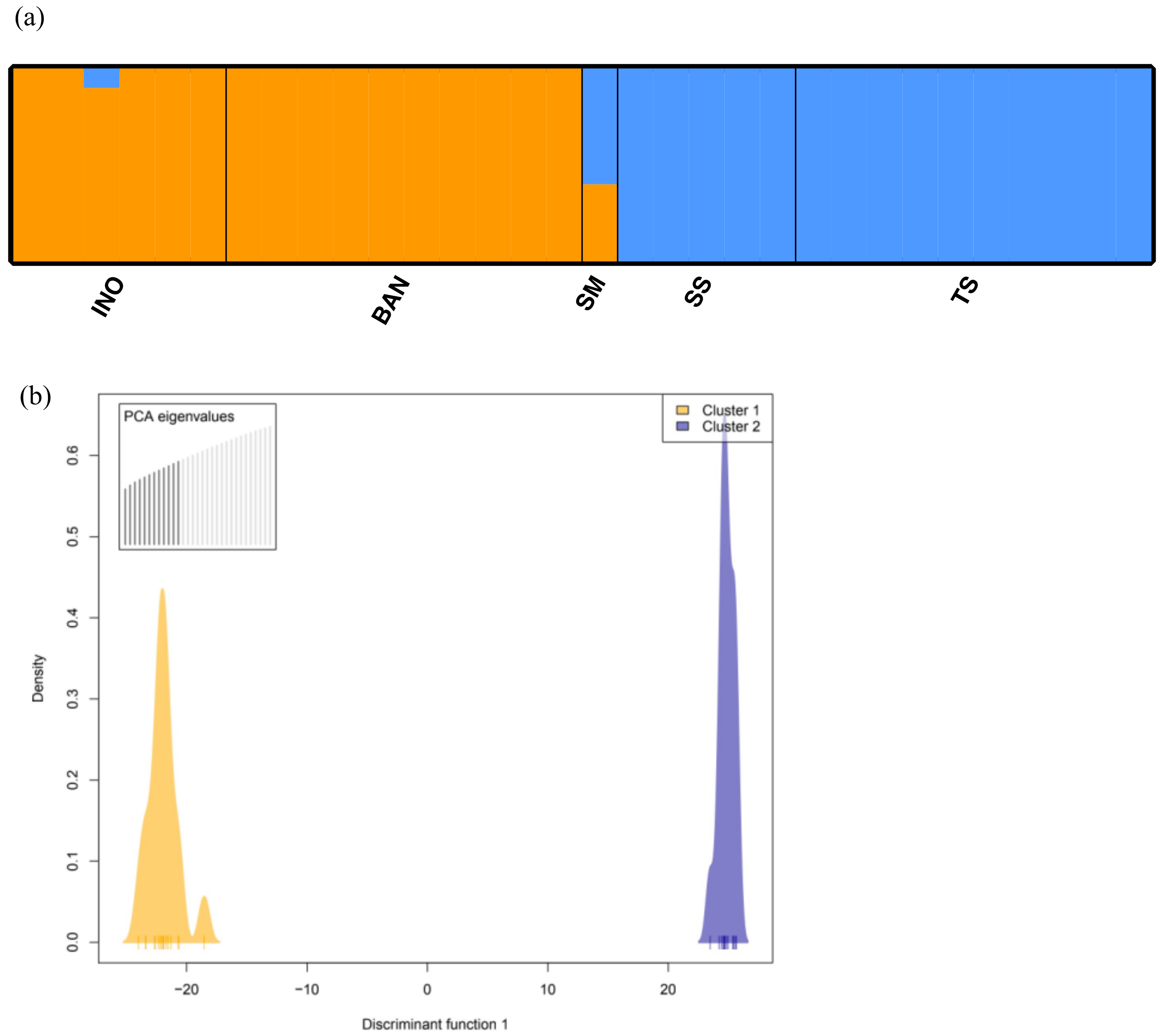
3.1. Population Structure

For P. chinensis, 6579 SNPs were used in STRUCTURE analysis after HWE testing and filtering to retain one SNP per locus. The highest delta K value was obtained when K equaled 2 (Figure S1a), which suggested that clustering into two groups was the best-fitting model to the observed data (Figure 2a). The result of DAPC analysis using 5282 SNPs was the same as STRUCTURE result in that the lowest BIC appeared when clustered into 2 groups (Figure S2a), that is, INO, BAN and SM in one group and SS and TS in the other (Figure 2b). The Π values of each population ranged from 0.102 to 0.141 (Table 2), with BAN having the lowest Π values. The mean pairwise FST values between populations ranged from 0.041 to 0.206 (Table 3). The mean pairwise FST values between populations within each ocean were smaller than cross oceans. The highest mean pairwise FST values was observed between BAN and SS with 0.206. After grouping the populations according to their ocean area, the pairwise FST values between the Pacific group and the Indian Ocean group was 0.131, indicating high genetic differentiation (Table 3).
For P. cinereus, 9488 SNPs were used in STRUCTURE analysis. The highest delta K value was obtained when K equaled 2 (Figure S1b), suggesting that two clusters is the best supported model (Figure 3a). The result of DAPC analysis using 7027 SNPs was different from the STRUCTURE result in that the lowest BIC appeared when the data were clustered into three groups (Figure S2b), counting IRAN as one group, INO and BAN as one group and SS and ES as another group (Figure 3b). The Π values for each population ranged from 0.049 to 0.103 (Table 2), with ES having the lowest Π values. The mean pairwise FST values between populations ranged from 0.020 to 0.186 (Table 3). Pairwise FST values between populations within oceans were smaller than cross oceans. The highest mean pairwise FST value was observed between IRAN and ES s 0.186. After grouping the populations according to their region, the pairwise FST values between the Pacific group and the western Indian Ocean group was 0.180, while 0.094 between the Pacific group and the eastern Indian Ocean group and 0.053 between the west Indian Ocean group and the east Indian Ocean group (Table 3).

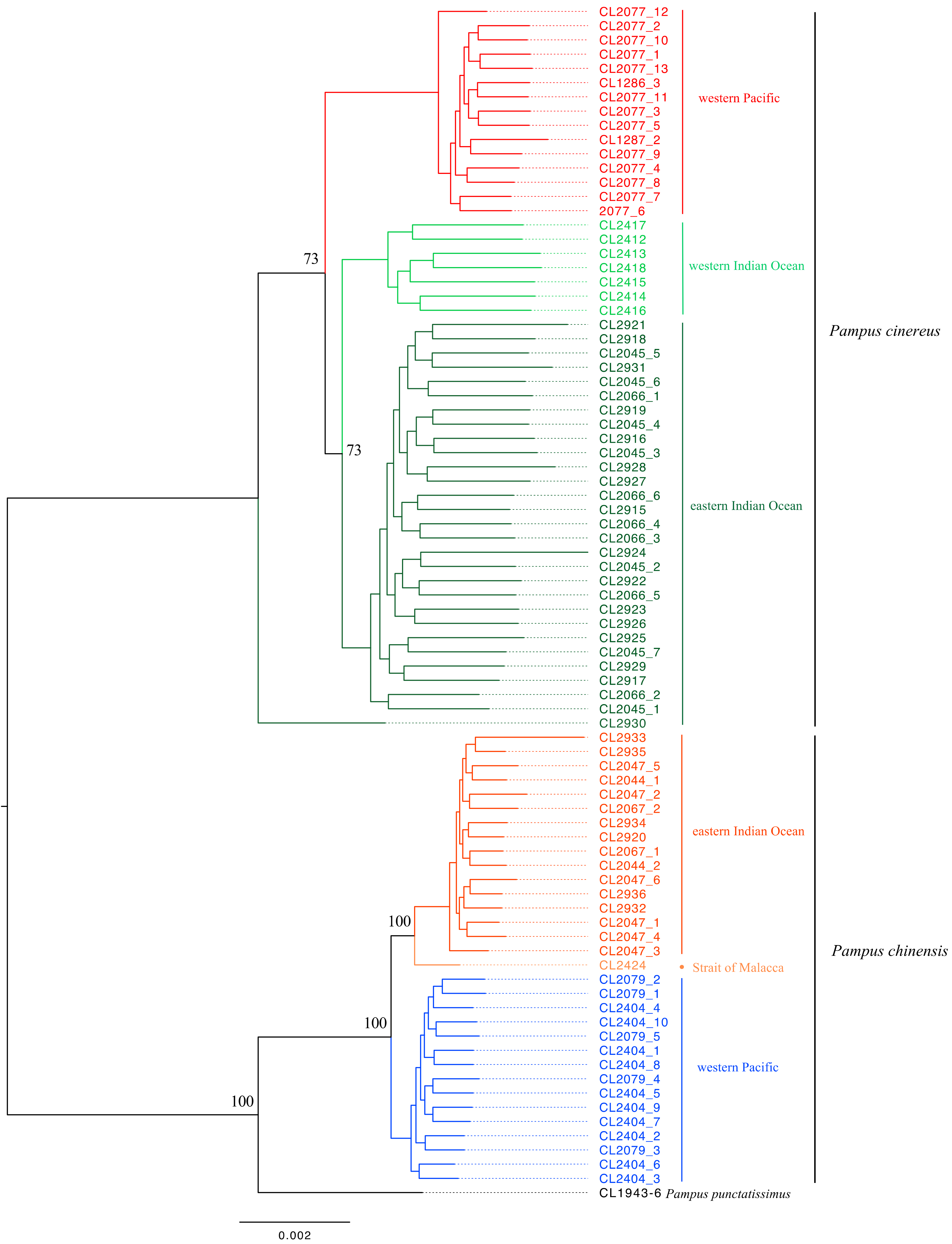
3.2. Phylogenetic Partitions

After filtering, 7379 genes were used to reconstruct the phylogenetic tree. In the concatenate tree reconstructed using RAXML, samples of individuals of P. chinensis collected from the western Pacific were clustered into one lineage while those from the Indian Ocean were clustered into another. The pattern of divergence within P. cinereus was similar as in P. chinensis, except that P. cinereus collected from the Indian Ocean were clustered into two sublineages, the eastern Indian Ocean and the western Indian Ocean (Figure 4). The coalescent-based species tree reconstructed using ASTRAL-III exhibited the same partitioning pattern for P. chinensis and P. cinereus (Figure S3).

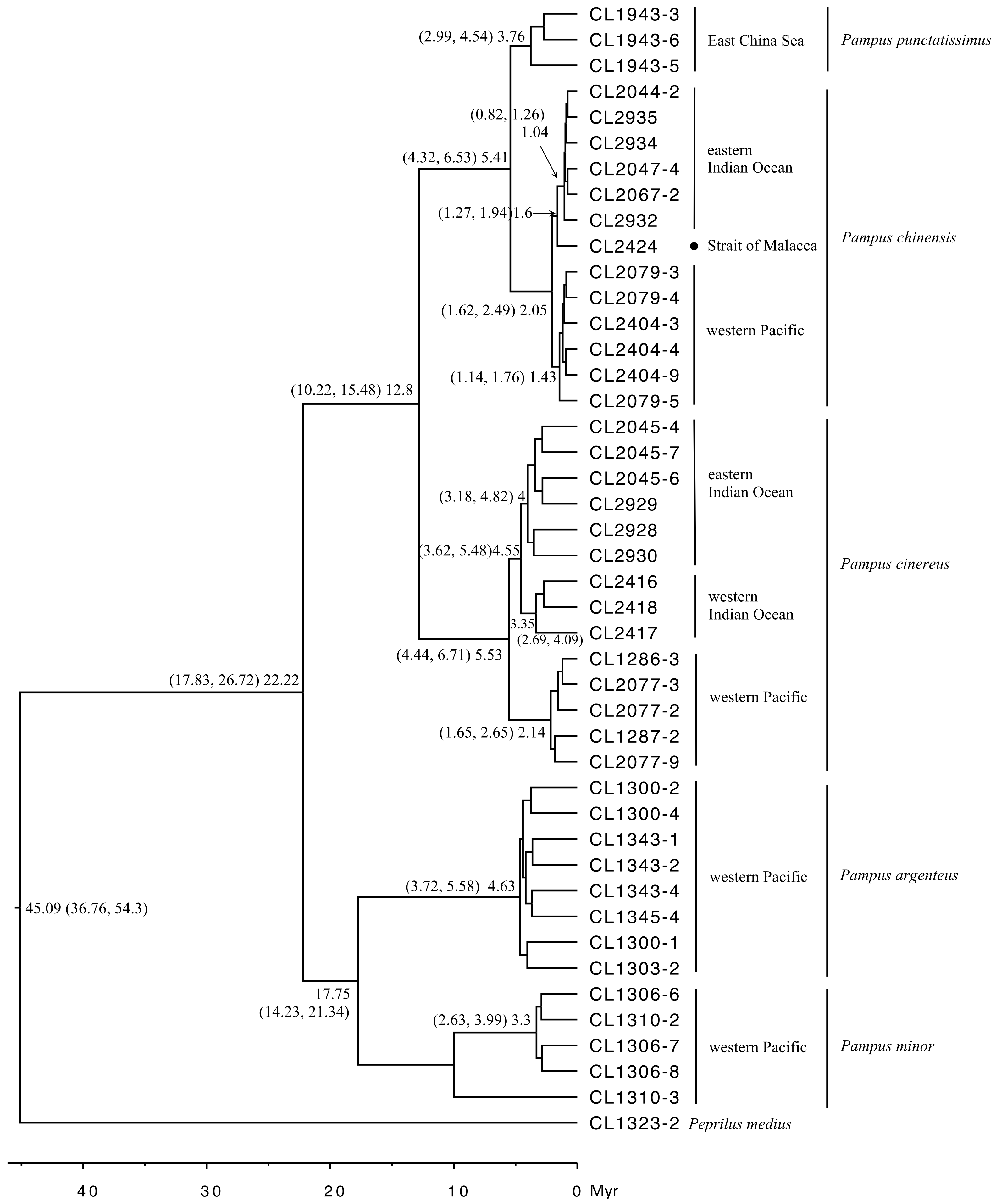
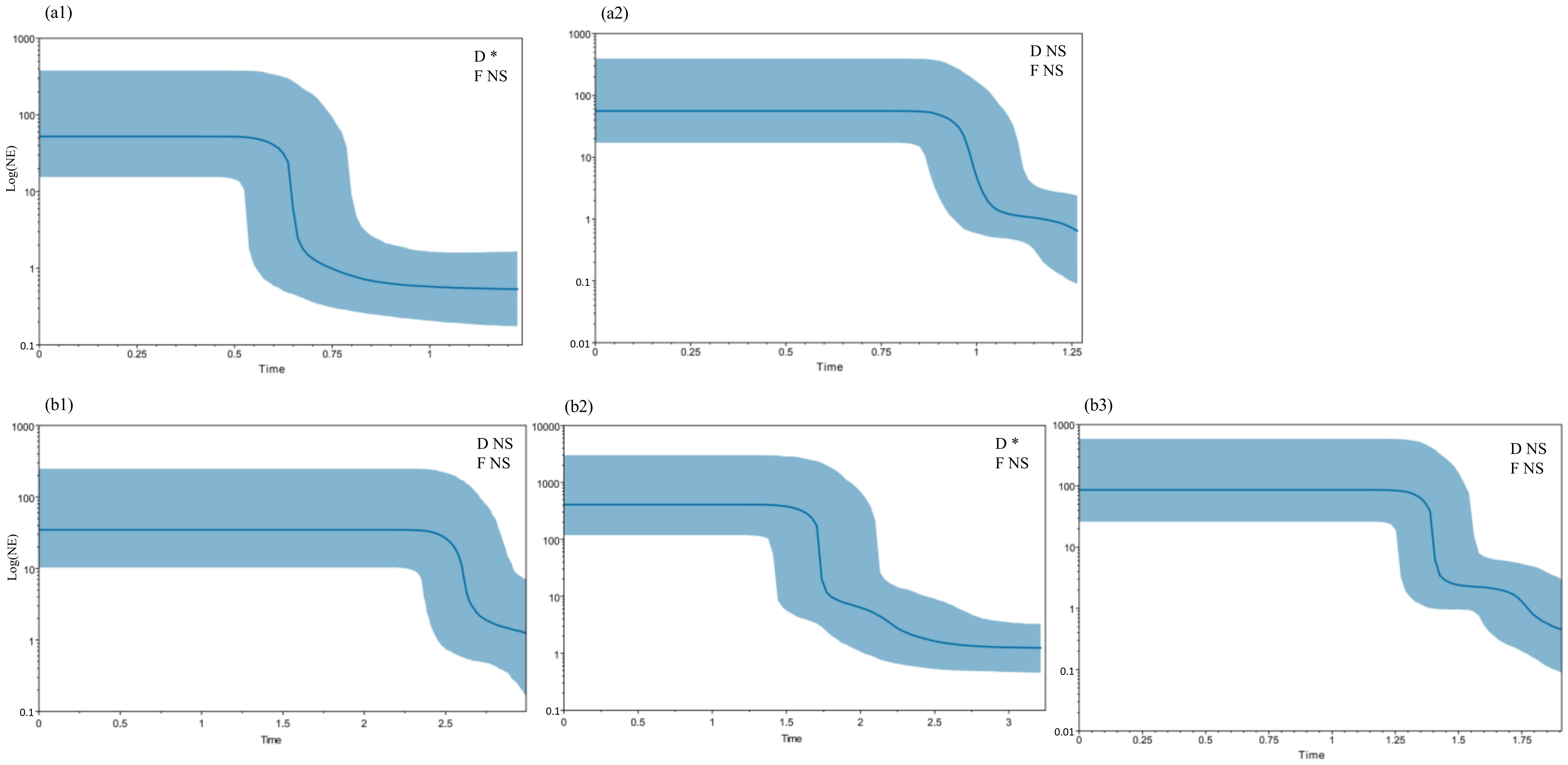
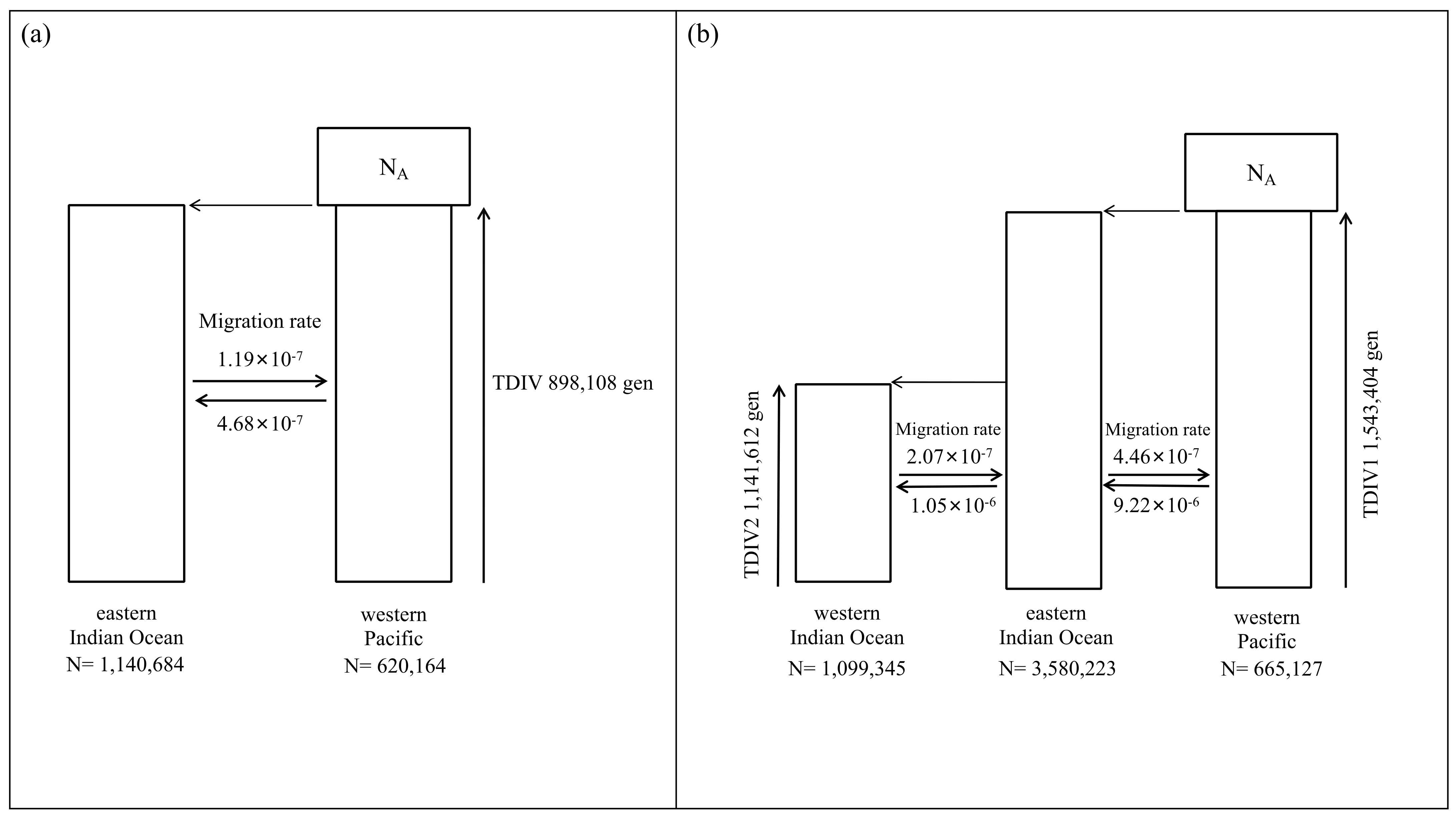
3.3. Divergence Time and Demographic History
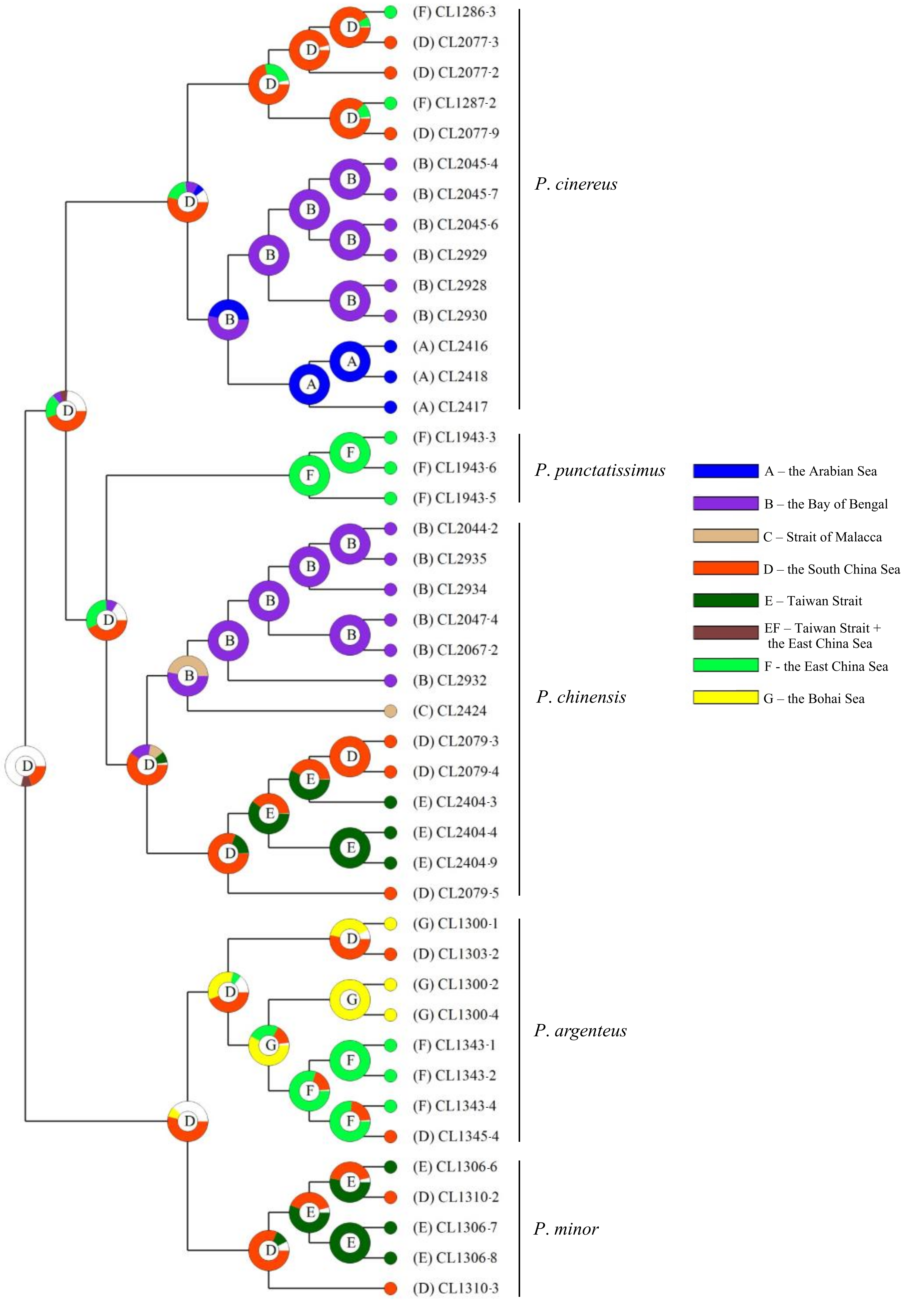
A total of 1437 loci were concatenated and used for estimation of divergence time. In the result, the estimated first occurrence of genus Pampus was in the early Miocene, ~22.22 Mya (CI 17.83–26.72, other CI of estimated divergence time see Figure 5). For the five species of genus Pampus, the estimated first occurrence of P. chinensis was ~2.05 Mya, P. cinereus was ~5.53 Mya, P. punctatissimus was ~3.76 Mya, P. argenteus was ~4.63 Mya, and P. minor was ~3.3 Mya. Particularly, for P. chinensis, the estimated first occurrence of the Indian Ocean and Pacific lineages were ~1.6 Mya and ~1.43 Mya, respectively. For P. cinereus, the Indian Ocean lineage was first occurred in ~4.55 Mya, and the Pacific was first occurred in ~2.14 Mya (Figure 5).
Bayesian skyline analysis showed that all lineages of both P. chinensis and P. cinereus have experienced a demographic plateau since population expansion and with a relatively low effective population size (Ne) except for the eastern Indian Ocean lineage of P. cinereus (Figure 6). Meanwhile, only the eastern Indian Ocean lineage of P. chinensis and the eastern Indian Ocean lineage of P. cinereus obtained significant negative value in Tajima’s D test but nonsignificant positive value in Fu’s Fs test, while other lineages obtained both the nonsignificant negative value in Tajima’s D test and positive value in Fu’s Fs test (Table S2).
In the FASTSIMCOAL2 analysis, a total of 5557 independent loci were used to generate folded SFS for P. chinensis. The best-fitting demographic model for P. chinensis was model 5, with the highest likelihood (Figure S4a) and lowest AIC (the second-best model ΔAIC = 84.62), indicating that the Pacific and the eastern Indian Ocean groups were divergent from a common ancestor around 898,108 generations ago (95% CI 888,139–917,095). Since the gene flow was estimated backward-in-time, the forward gene flow should be as the same value but reversed in direction. In this context, estimated gene flow from the Pacific to the eastern Indian Ocean (4.58 × 10⁻⁷, 95% CI 4.43 × 10⁻⁷–4.66 × 10⁻⁷) was stronger than that from the eastern Indian Ocean to the Pacific (1.19 × 10⁻⁷, 95% CI 1.12 × 10⁻⁷–1.23 × 10⁻⁷; Figure 7a). For P. cinereus, a total of 7222 independent loci were used to generate folded SFS. The likelihood distribution of model 6 and model 8 overlapped (Figure S4b); however, model 6 had a lower AIC than model 8 (ΔAIC = 10.32). Hence, model 6 was chosen, indicating that the Pacific group and the eastern Indian Ocean group were divergent from a common ancestor 1,543,404 generations ago (95% CI 1,417,135–1,659,188), and after a few generations (1,141,612 generations ago, 95% CI 1,141,526–1,321,759). The western Indian Ocean group diverged from the eastern Indian group, and gene flow persisted within and between oceans. The estimated forward-in-time gene flow from the Pacific to the eastern Indian Ocean (9.22 × 10⁻⁶, 95% CI 0–9.79 × 10⁻⁶) was stronger than that from the eastern Indian Ocean to the Pacific (4.46 × 10⁻⁷, 95% CI 0–1.29 × 10⁻⁵). Moreover, the gene flow from the eastern Indian Ocean to the western Indian Ocean (1.05 × 10⁻⁶, 95% CI 0–3.11 × 10⁻⁵) was stronger than the reverse direction (2.07 × 10⁻⁷, 95% CI 9.19 × 10⁻⁸–2.75 × 10⁻⁵; Figure 7b).

3.4. Ancestral Area

The best-supported model for ancestral area reconstruction was Dispersal–Extinction–Cladogenesis + jump dispersal (DEC + j), which means the ancestor of Pampus could undergo all kinds of anagenetic (dispersal, extinction) and cladogenetic (narrow-, full-sympatry or allopatry, etc.) events [63,64]. In the analysis, 15 dispersal and vicariance events were inferred within the genus Pampus, and the results suggested that the South China Sea was the ancestral area for genus Pampus (Figure 8).

4. Discussion

4.1. Intraspecific Diversification of P. chinensis and P. cinereus

Interoceanic differentiation was detected within both P. chinensis and P. cinereus. In the results of STRUCTURE analysis, P. chinensis clustered into two groups, and the same result was found for P. cinereus. The DAPC analysis showed similar results, except that P. cinereus was further split into three clusters. The clustering of these two species was similar, according to oceanic areas, suggesting that the IPB acted as a barrier between the Indian Ocean and the western Pacific for a long enough time to derive genetic differentiation. The same effect was observed in other marine taxa that are distributed among the Pacific and the Indian Ocean, such as Labroides dimidiatus, Plectroglyphidodon lacrymatus, Sargocentron diadema, etc. [65]. Some differences also were seen in the FST statistics results. When we grouped the populations according to their oceanic areas, P. chinensis showed a large differentiation between the eastern Indian Ocean and the western Pacific, but P. cinereus showed a medium level of differentiation between the eastern Indian Ocean and the western Pacific, and large differentiation between the western Indian Ocean and the western Pacific, which indicated that P. cinereus may be further diverged due to the barrier of the Indian subcontinent.
The partitioning patterns also were observed in the phylogenetic tree, which explicitly divided into the Indian Ocean lineage and the western Pacific lineage (Figure 4) for each species. Interestingly, the sample of P. chinensis from the Strait of Malacca was diverged from other individuals of the Indian Ocean lineage (Figure 4), and STRUCTURE analysis indicated that its genetic variants were roughly half from the Indian Ocean and half from the western Pacific (Figure 2a). Since this sampling location was near the IPB, hybridization may have happened between the individuals from the eastern Indian Ocean and western Pacific to form a hybrid population; however, more individuals should be sampled from this location to provide robust evidence. P. cinereus of the Indian Ocean lineage was separated into the western Indian Ocean lineage and the eastern Indian Ocean lineage, which may be a consequence of the isolation between the Arabian Sea and the Bay of Bengal. Divya et al. [20] reported that Pampus species collected from the Arabian Sea and the Bay of Bengal have affinity to P. cinereus collected from the South China Sea. In their COI tree, these three populations were clustered into three lineages, which was the same as our topology. Combining the results based on mitochondrial DNA and nuclear DNA, respectively, we suggest that three lineages exist within P. cinereus. Divya et al. [21] described the Pampus species collected from the Arabian Sea as a new species, P. candidus, but we think further scrutiny should be made to split more species from P. cinereus lineages before distinct morphological characters are identified. On the other hand, P. liuorum, a controversial Pampus species, was defined as a synonym of P. cinereus in our previous study [15], but a recent study justified P. liuorum as a valid species using two mitochondrial DNA barcodes [66]. In their Cytb trees, P. cinereus and P. liuroum sampled in the western Pacific were separated in two lineages, which was different from our result, but their COI tree corroborated our result that P. cinereus and P. liuroum are not reciprocal in monophyletic. More comparison of specimens and integrated data sets should be collected to assess the status of P. liuroum. Nevertheless, our results suggest that the IPB is a major factor diversifying P. chinensis and P. cinereus, both of which consist of an Indian Ocean lineage and a Pacific lineage.

4.2. The Mechanism of Forming Different Intraspecific Lineages

Since the IPB has shown its barrier effect on P. chinensis and P. cinereus, exploring the mechanism of how P. chinensis and P. cinereus formed into different lineages is meaningful. Due to glaciation in the Pleistocene, the sea level was below its present level by as much as 120 m [67], and there have been at least eight 100 thousand-year cycles [68]. In these periods, the Sunda Shelf, which forms the IPB, was mostly exposed, restricting exchange between the western Pacific and the tropical Indian Ocean [2]. Estimated time-tree showed that the occurrence of each lineage of P. chinensis was in the mid-late Pleistocene, and lineages of P. cinereus were in the early Pleistocene or even late Pliocene. We hypothesize that divergence between oceans of both P. chinensis and P. cinereus were due to sea level fluctuations caused by repeated glaciation in the Pleistocene that isolated the populations in these two ocean areas for a long time. Combining the results, we propose these scenarios for species divergence: (1) for P. chinensis, ~2 million years ago from the South China Sea, the common ancestor of the Indian Ocean and Pacific lineages started to disperse and then diverged. Temperature dropped sharply after the new populations colonized the eastern Indian Ocean and western Pacific, dropping the sea level below the then-present level and the IPB isolated the two new populations until the end of the ice age. Due to a long time of geographic isolation, the Indian and Pacific lineages were formed and subsequently restored a low-level of gene flow between the two oceans until present. (2) The divergence of P. cinereus was similar to the scenario of P. chinensis, as though it occurred in an earlier age. The common ancestor of the western and eastern Indian Ocean lineages and Pacific lineage dispersed from the South China Sea, and they first colonized in the eastern Indian Ocean and then the western Indian Ocean. Similarly, the mostly exposed Sunda Shelf interrupted gene flow between the Indian Ocean and Pacific and formed the Indian lineage and Pacific lineage. The genetic breaks caused by the IPB are also reported in other marine organisms [69]. However, in the Indian Ocean lineage, there are sublineages in the western Indian Ocean and the eastern Indian Ocean. We suggest this should not be affected by the glaciations but maybe the founder effect. Meanwhile, only both the eastern Indian Ocean lineages of P. chinensis and P. cinereus obtained significant negative Tajima’s D values; combining the Bayesian skyline plots result, we suggest all lineages of P. chinensis and P. cinereus are experiencing a demographic plateau period since diverging expansion.
FASTSIMCOAL2 results estimated that divergences between the Indian Ocean and Pacific lineages of P. chinensis and P. cinereus were 898,108 generations ago and 1,543,404 generations ago, respectively. Previous studies reported that P. argenteus spawns twice a year [16], and all individuals in a population reach sexual maturity in two years [70]. Since the reproductive biological characteristics are similar within the genus [17], the generation times of P. chinensis and P. cinereus were set to 2 years. Therefore, the divergence between the Indian Ocean lineage and Pacific lineage of P. chinensis and P. cinereus should be around 1,796,216 years ago and 3,086,808 years ago, respectively. The estimated time frame overlaps with the result of our reconstructed time-tree. In other words, this result also suggests that the low sea level in the Pleistocene may have caused the diversification within both P. chinensis and P. cinereus between the western Pacific and the Indian Ocean.

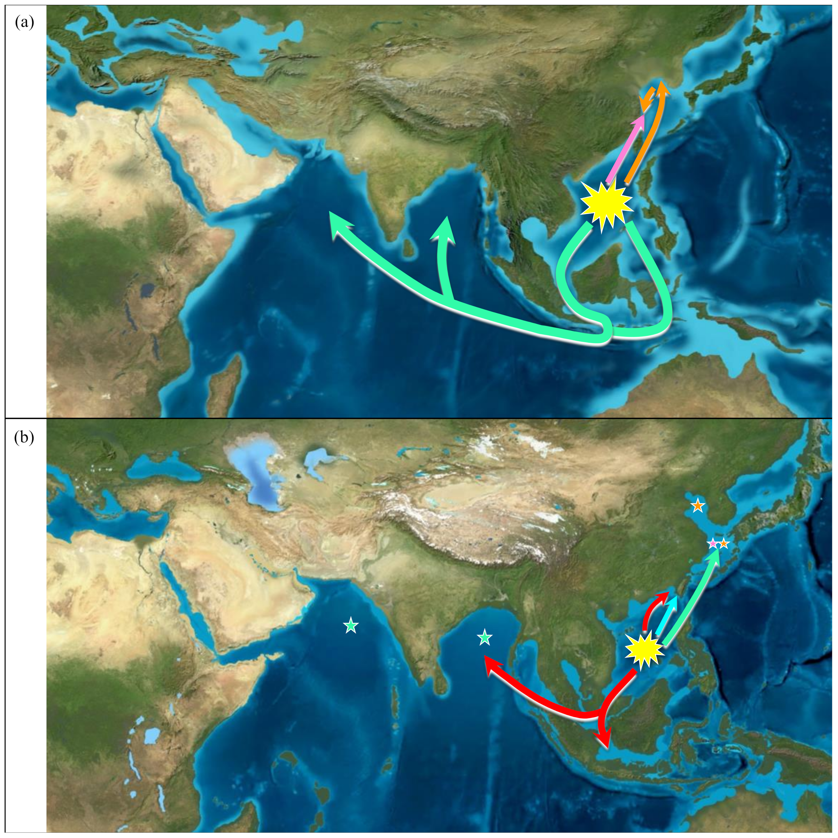
4.3. The Origin and Dispersal Routes of Genus Pampus

The time-tree estimated that the common ancestor of all Pampus species lived ~22.22 Mya, a period of explosive diversification in most modern marine fishes [13]. Our result suggests that dispersals and diversifications were carried on subsequently. The first species appearing was P. cinereus in the South China Sea, and then it began westward dispersal to the eastern Indian Ocean and then the western Indian Ocean and northward dispersal to the East China Sea. The second species diverging was P. argenteus in the South China Sea, and then it began dispersal to the Bohai Sea and then colonized the East China Sea. P. punctatissimus and P. minor appeared almost at the same time, while P. punctatissimus dispersed northward to the East China Sea and P. minor northward to the Taiwan Strait. The most modern Pampus species is P. chinensis that first appeared in the South China Sea and then began to disperse westward to the eastern Indian Ocean and northward to the Taiwan Strait (Figure 9). The dispersal routes may have been facilitated by the ocean currents in the western Pacific and north Indian Ocean. We suggest that the South China Sea southern cyclonic gyre [71] would facilitate the individuals through the shallow sea strait and reach the eastern Indian Ocean, and then the Monsoon Current in the north Indian Ocean [72] would facilitate further westward dispersal. The Guangdong Coastal Current, South China Sea Warm Current, South China Sea Branch of Kuroshio and Luzon cyclonic gyre [71] would facilitate individuals through the Taiwan Strait and Luzon Strait, and then the Kuroshio Current [73] would facilitate further northward dispersal.
The Indo–Australian Archipelago, also known as the Coral Triangle (CT), is a marine biodiversity center which contains numerous marine species [5]. Three hypotheses were proposed to explain the high biodiversity in the CT: center of origin, center of overlap and center of accumulation. Although Bellwood and Meyer [74] suggested the center of accumulation model could best describe the high biodiversity in CT, Briggs [75] proposed that the species accumulation that happened in the Eocene of the West Tethys and CT had its ability to produce species after the early Miocene. In our results, the occurrence and most probable origin of genus Pampus were estimated to be the early Miocene (~22.22 Mya) in the South China Sea, which is near the CT. Thus, our results provide new evidence for the center of origin model for CT and emphasize the CT as an important region for biodiversity conservation.

Supplementary Materials

The following are available online at https://www.mdpi.com/article/10.3390/d14030180/s1, Figure S1: Mean log-likelihood Pr (X|K) and delta K, Figure S2: BIC values for each cluster, Figure S3: Coalescent-based species tree, Figure S4: Likelihood distributions for different models, Table S1: Numbers of enriched genes for each individual, Table S2: Values of Tajima’s D test and Fu’s Fs test.

Author Contributions

C.L. conceived this study and collected the samples. G.Y. and A.S. collected the samples. G.F. conducted the experiments, analyzed the data and wrote the manuscript. All authors discussed the results and edited the final manuscript. All authors have read and agreed to the published version of the manuscript.

Funding

This work was supported by “Science and Technology Commission of Shanghai Municipality (19050501900)” to C.L.

Institutional Review Board Statement

The study was approved by the Animal Care and Use Committee of Shanghai Ocean University. Experiment procedures were performed in accordance with the Provisions and Regulations for the National Experimental Animal Management Regulations (China, July, 2013).

Informed Consent Statement

Not applicable.

Data Availability Statement

The raw FASTQ reads are available in the NCBI repository with accession number PRJNA809874. All scripts used in this study were deposited in a GitHub repository (link to this repository: https://github.com/naFgG/Scripts_used_in_Pampus, 23 February 2022).

Acknowledgments

We are grateful to Leyli Purrafee Dizaj, Sekar Megarajan, and Suhan Liu for helping with sample collection. We would also like to thank Shanghai Oceanus Supercomputing Center (SOSC) for providing computational resource.

Conflicts of Interest

The authors declare no conflict of interest.

References

  1. Briggs, J.C.; Bowen, B.W. A realignment of marine biogeographic provinces with particular reference to fish distributions. J. Biogeogr. 2012, 39, 12–30. [Google Scholar] [CrossRef]
  2. Bowen, B.W.; Gaither, M.R.; DiBattista, J.D.; Iacchei, M.; Andrews, K.R.; Grant, W.S.; Toonen, R.J.; Briggs, J.C. Comparative phylogeography of the ocean planet. Proc. Natl. Acad. Sci. USA 2016, 113, 7962–7969. [Google Scholar] [CrossRef] [Green Version]
  3. Waldrop, E.; Hobbs, J.P.A.; Randall, J.E.; DiBattista, J.D.; Rocha, L.A.; Kosaki, R.K.; Berumen, M.L.; Bowen, B.W. Phylogeography, population structure and evolution of coral-eating butterflyfishes (Family Chaetodontidae, genus Chaetodon, subgenus Corallochaetodon). J. Biogeogr. 2016, 43, 1116–1129. [Google Scholar] [CrossRef] [Green Version]
  4. Ahti, P.A.; Coleman, R.R.; DiBattista, J.D.; Berumen, M.L.; Rocha, L.A.; Bowen, B.W. Phylogeography of Indo-Pacific reef fishes: Sister wrasses Coris gaimard and C. cuvieri in the Red Sea, Indian Ocean and Pacific Ocean. J. Biogeogr. 2016, 43, 1103–1115. [Google Scholar] [CrossRef]
  5. Gaither, M.R.; Bowen, B.W.; Bordenave, T.R.; Rocha, L.A.; Newman, S.J.; Gomez, J.A.; van Herwerden, L.; Craig, M.T. Phylogeography of the reef fish Cephalopholis argus (Epinephelidae) indicates Pleistocene isolation across the Indo-Pacific Barrier with contemporary overlap in The Coral Triangle. BMC Evol. Biol. 2011, 11, 189. [Google Scholar] [CrossRef] [Green Version]
  6. Craig, M.T.; Eble, J.A.; Bowen, B.W.; Robertson, D.R. High genetic connectivity across the Indian and Pacific Oceans in the reef fish Myripristis berndti (Holocentridae). Mar. Ecol. Prog. Ser. 2007, 334, 245–254. [Google Scholar] [CrossRef] [Green Version]
  7. Gaither, M.R.; Toonen, R.J.; Robertson, D.R.; Planes, S.; Bowen, B.W. Genetic evaluation of marine biogeographical barriers: Perspectives from two widespread Indo-Pacific snappers (Lutjanus kasmira and Lutjanus fulvus). J. Biogeogr. 2010, 37, 133–147. [Google Scholar] [CrossRef]
  8. Duncan, K.M.; Martin, A.P.; Bowen, B.W.; De Couet, H.G. Global phylogeography of the scalloped hammerhead shark (Sphyrna lewini). Mol. Ecol. 2006, 15, 2239–2251. [Google Scholar] [CrossRef]
  9. Reece, J.S.; Bowen, B.W.; Joshi, K.; Goz, V.; Larson, A. Phylogeography of two moray eels indicates high dispersal throughout the indo-pacific. J. Hered. 2010, 101, 391–402. [Google Scholar] [CrossRef] [Green Version]
  10. Horne, J.B.; van Herwerden, L.; Choat, J.H.; Robertson, D.R. High population connectivity across the Indo-Pacific: Congruent lack of phylogeographic structure in three reef fish congeners. Mol. Phylogenetics Evol. 2008, 49, 629–638. [Google Scholar] [CrossRef]
  11. Ma, K.Y.; van Herwerden, L.; Newman, S.J.; Berumen, M.L.; Choat, J.H.; Chu, K.H.; de Mitcheson, Y.S. Contrasting population genetic structure in three aggregating groupers (Percoidei: Epinephelidae) in the Indo-West Pacific: The importance of reproductive mode. BMC Evol. Biol. 2018, 18, 180. [Google Scholar] [CrossRef]
  12. Taillebois, L.; Castelin, M.; Ovenden, J.R.; Bonillo, C.; Keith, P. Contrasting Genetic Structure among Populations of Two Amphidromous Fish Species (Sicydiinae) in the Central West Pacific. PLoS ONE 2013, 8, e75465. [Google Scholar] [CrossRef] [Green Version]
  13. Li, C.Y.; Olave, M.; Hou, Y.L.; Qin, G.; Schneider, R.F.; Gao, Z.X.; Tu, X.L.; Wang, X.; Qi, F.R.; Nater, A.; et al. Genome sequences reveal global dispersal routes and suggest convergent genetic adaptations in seahorse evolution. Nat. Commun. 2021, 12, 1–11. [Google Scholar] [CrossRef] [PubMed]
  14. Qiu, F.; Li, H.; Lin, H.; Ding, S.; Miyamoto, M.M. Phylogeography of the inshore fish, Bostrychus sinensis, along the Pacific coastline of China. Mol. Phylogenetics Evol. 2016, 96, 112–117. [Google Scholar] [CrossRef]
  15. Yin, G.; Pan, Y.; Anirban, S.; Mohammad, A.B.; Kim, J.-K.; Wu, H.; Li, C. Molecular systematics of Pampus (Perciformes: Stromateidae) based on thousands of nuclear loci using target-gene enrichment. Mol. Phylogenetics Evol. 2019, 140, 106595. [Google Scholar] [CrossRef]
  16. Almatar, S.M.; Lone, K.P.; Abu-Rezq, T.S.; Yousef, A.A. Spawning frequency, fecundity, egg weight and spawning type of silver pomfret, Pampus argenteus (Euphrasen) (Stromateidae), in Kuwait waters. J. Appl. Ichthyol. 2004, 20, 176–188. [Google Scholar] [CrossRef]
  17. Shi, Z.H.; Peng, S.M.; Sun, P.; Yin, F. Developmental potential and prospect of Pampus culture in China. Mod. Fish. Inf. 2009, 24, 3–4. [Google Scholar] [CrossRef]
  18. Liu, J.; Li, C.; Li, X. Phylogeny and biogeography of Chinese pomfret fishes (Pisces: Stromateidae). Studia Mar. Sin. 2002, 44, 235–239. [Google Scholar]
  19. Liu, J.; Li, C.S.; Ning, P. A redescription of grey pomfret Pampus cinereus (Bloch, 1795) with the designation of a neotype (Teleostei: Stromateidae). Chin. J. Oceanol. Limnol. 2013, 31, 140–145. [Google Scholar] [CrossRef]
  20. Divya, P.R.; Mohitha, C.; Rahul, G.K.; Shanis, C.P.R.; Basheer, V.S.; Gopalakrishnan, A. Molecular based phylogenetic species recognition in the genus Pampus (Perciformes: Stromateidae) reveals hidden diversity in the Indian Ocean. Mol. Phylogenetics Evol. 2017, 109, 240–245. [Google Scholar] [CrossRef]
  21. Divya, P.R.; Rahul, G.K.; Chelat, M.; Shanis, C.P.R.; Bineesh, K.K.; Basheer, V.S.; Achamveetil, G. Resurrection and Re-description of Pampus candidus (Cuvier), Silver Pomfret from the Northern Indian Ocean. Zool. Stud. 2019, 58, e7. [Google Scholar] [CrossRef]
  22. Li, Y.; Gao, T.X.; Zhou, Y.D.; Lin, L.S. Spatial genetic subdivision among populations of Pampus chinensis between China and Pakistan: Testing the barrier effect of the Malay Peninsula. Aquat. Living Resour. 2019, 32, 8. [Google Scholar] [CrossRef]
  23. Li, C.; Hofreiter, M.; Straube, N.; Corrigan, S.; Naylor, G.J. Capturing protein-coding genes across highly divergent species. Biotechniques 2013, 54, 321–326. [Google Scholar] [CrossRef]
  24. Meyer, M.; Kircher, M. Illumina sequencing library preparation for highly multiplexed target capture and sequencing. Cold Spring Harb. Protoc. 2010, 2010, 5448. [Google Scholar] [CrossRef]
  25. Fisher, S.; Barry, A.; Abreu, J.; Minie, B.; Nolan, J.; Delorey, T.M.; Young, G.; Fennell, T.J.; Allen, A.; Ambrogio, L.; et al. A scalable, fully automated process for construction of sequence-ready human exome targeted capture libraries. Genome Biol. 2011, 12, R1. [Google Scholar] [CrossRef] [Green Version]
  26. Song, S.; Zhao, J.; Li, C. Species delimitation and phylogenetic reconstruction of the sinipercids (Perciformes: Sinipercidae) based on target enrichment of thousands of nuclear coding sequences. Mol. Phylogenetics Evol. 2017, 111, 44–55. [Google Scholar] [CrossRef]
  27. Marcel, M. Cutadapt removes adapter sequences from high-throughput sequencing reads. EMBnet. J. 2011, 17, 10–12. [Google Scholar] [CrossRef]
  28. Yuan, H.; Atta, C.; Tornabene, L.; Li, C. Assexon: Assembling Exon Using Gene Capture Data. Evol Bioinform. 2019, 15, 1–13. [Google Scholar] [CrossRef]
  29. Jared, T.S.; Richard, D. Efficient de novo assembly of large genomes using compressed data structures. Genome Res. 2012, 22, 14. [Google Scholar] [CrossRef] [Green Version]
  30. Katoh, K.; Standley, D.M. MAFFT multiple sequence alignment software version 7: Improvements in performance and usability. Mol. Biol. Evol. 2013, 30, 772–780. [Google Scholar] [CrossRef] [Green Version]
  31. Yuan, H.; Jiang, J.; Jimenez, F.A.; Hoberg, E.P.; Cook, J.A.; Galbreath, K.E.; Li, C. Target gene enrichment in the cyclophyllidean cestodes, the most diverse group of tapeworms. Mol. Ecol. Resour 2016, 16, 1095–1106. [Google Scholar] [CrossRef]
  32. Li, H.; Durbin, R. Fast and accurate short read alignment with Burrows-Wheeler transform. Bioinformatics 2009, 25, 1754–1760. [Google Scholar] [CrossRef] [Green Version]
  33. Li, H.; Handsaker, B.; Wysoker, A.; Fennell, T.; Ruan, J.; Homer, N.; Marth, G.; Abecasis, G.; Durbin, R.; Proc, G.P.D. The Sequence Alignment/Map format and SAMtools. Bioinformatics 2009, 25, 2078–2079. [Google Scholar] [CrossRef] [Green Version]
  34. Li, H. Aligning sequence reads, clone sequences and assemly contigs with BWA-MEM. arXiv 2013, arXiv:1303.3997. [Google Scholar]
  35. McKenna, A.; Hanna, M.; Banks, E.; Sivachenko, A.; Cibulskis, K.; Kernytsky, A.; Garimella, K.; Altshuler, D.; Gabriel, S.; Daly, M.; et al. The Genome Analysis Toolkit: A MapReduce framework for analyzing next-generation DNA sequencing data. Genome Res. 2010, 20, 1297–1303. [Google Scholar] [CrossRef] [Green Version]
  36. Danecek, P.; Auton, A.; Abecasis, G.; Albers, C.A.; Banks, E.; DePristo, M.A.; Handsaker, R.E.; Lunter, G.; Marth, G.T.; Sherry, S.T.; et al. The variant call format and VCFtools. Bioinformatics 2011, 27, 2156–2158. [Google Scholar] [CrossRef]
  37. Pritchard, J.K.; Stephens, M.; Donnelly, P. Inference of population structure using multilocus genotype data. Genetics 2000, 155, 945–959. [Google Scholar] [CrossRef]
  38. Earl, D.A.; Vonholdt, B.M. Structure Harvester: A website and program for visualizing structure output and implementing the Evanno method. Conserv. Genet. Resour. 2012, 4, 359–361. [Google Scholar] [CrossRef]
  39. Jakobsson, M.; Rosenberg, N.A. CLUMPP: A cluster matching and permutation program for dealing with label switching and multimodality in analysis of population structure. Bioinformatics 2007, 23, 1801–1806. [Google Scholar] [CrossRef] [Green Version]
  40. Rosenberg, N.A. Distruct: A program for the graphical display of population structure. Mol. Ecol. Notes 2004, 4, 137–138. [Google Scholar] [CrossRef]
  41. Jombart, T.; Ahmed, I. Adegenet 1.3-1: New tools for the analysis of genome-wide SNP data. Bioinformatics 2011, 27, 3070–3071. [Google Scholar] [CrossRef] [PubMed] [Green Version]
  42. Catchen, J.; Hohenlohe, P.A.; Bassham, S.; Amores, A.; Cresko, W.A. Stacks: An analysis tool set for population genomics. Mol. Ecol. 2013, 22, 3124–3140. [Google Scholar] [CrossRef] [Green Version]
  43. Catchen, J.M.; Amores, A.; Hohenlohe, P.; Cresko, W.; Postlethwait, J.H. Stacks: Building and genotyping Loci de novo from short-read sequences. G3 (Bethesda) 2011, 1, 171–182. [Google Scholar] [CrossRef] [PubMed] [Green Version]
  44. Kuang, T.; Tornabene, L.; Li, J.; Jiang, J.; Chakrabarty, P.; Sparks, J.S.; Naylor, G.J.P.; Li, C. Phylogenomic analysis on the exceptionally diverse fish clade Gobioidei (Actinopterygii: Gobiiformes) and data-filtering based on molecular clocklikeness. Mol. Phylogenetics Evol. 2018, 128, 192–202. [Google Scholar] [CrossRef]
  45. Stamatakis, A. RAxML version 8: A tool for phylogenetic analysis and post-analysis of large phylogenies. Bioinformatics 2014, 30, 1312–1313. [Google Scholar] [CrossRef]
  46. Mirarab, S.; Reaz, R.; Bayzid, M.S.; Zimmermann, T.; Swenson, M.S.; Warnow, T. ASTRAL: Genome-scale coalescent-based species tree estimation. Bioinformatics 2014, 30, i541–i548. [Google Scholar] [CrossRef] [PubMed] [Green Version]
  47. Zhang, C.; Rabiee, M.; Sayyari, E.; Mirarab, S. ASTRAL-III: Polynomial time species tree reconstruction from partially resolved gene trees. BMC Bioinform. 2018, 19, 153. [Google Scholar] [CrossRef] [Green Version]
  48. Minh, B.Q.; Schmidt, H.A.; Chernomor, O.; Schrempf, D.; Woodhams, M.D.; von Haeseler, A.; Lanfear, R. IQ-TREE 2: New Models and Efficient Methods for Phylogenetic Inference in the Genomic Era. Mol. Biol. Evol. 2020, 37, 1530–1534. [Google Scholar] [CrossRef] [Green Version]
  49. Kalyaanamoorthy, S.; Minh, B.Q.; Wong, T.K.F.; von Haeseler, A.; Jermiin, L.S. ModelFinder: Fast model selection for accurate phylogenetic estimates. Nat. Methods 2017, 14, 587–589. [Google Scholar] [CrossRef] [Green Version]
  50. Hoang, D.T.; Chernomor, O.; von Haeseler, A.; Minh, B.Q.; Vinh, L.S. UFBoot2: Improving the Ultrafast Bootstrap Approximation. Mol. Biol. Evol. 2018, 35, 518–522. [Google Scholar] [CrossRef]
  51. Bouckaert, R.; Vaughan, T.G.; Barido-Sottani, J.; Duchene, S.; Fourment, M.; Gavryushkina, A.; Heled, J.; Jones, G.; Kuhnert, D.; De Maio, N.; et al. BEAST 2.5: An advanced software platform for Bayesian evolutionary analysis. PLoS Comput. Biol. 2019, 15, e1006650. [Google Scholar] [CrossRef] [Green Version]
  52. Heled, J.; Drummond, A.J. Calibrated tree priors for relaxed phylogenetics and divergence time estimation. Syst. Biol. 2012, 61, 138–149. [Google Scholar] [CrossRef] [PubMed] [Green Version]
  53. Miya, M.; Friedman, M.; Satoh, T.P.; Takeshima, H.; Sado, T.; Iwasaki, W.; Yamanoue, Y.; Nakatani, M.; Mabuchi, K.; Inoue, J.G.; et al. Evolutionary origin of the Scombridae (tunas and mackerels): Members of a paleogene adaptive radiation with 14 other pelagic fish families. PLoS ONE 2013, 8, e73535. [Google Scholar] [CrossRef] [PubMed]
  54. Rabosky, D.L.; Chang, J.; Title, P.O.; Cowman, P.F.; Sallan, L.; Friedman, M.; Kaschner, K.; Garilao, C.; Near, T.J.; Coll, M.; et al. An inverse latitudinal gradient in speciation rate for marine fishes. Nature 2018, 559, 392–395. [Google Scholar] [CrossRef]
  55. Rabosky, D.L.; Santini, F.; Eastman, J.; Smith, S.A.; Sidlauskas, B.; Chang, J.; Alfaro, M.E. Rates of speciation and morphological evolution are correlated across the largest vertebrate radiation. Nat. Commun. 2013, 4, 1958. [Google Scholar] [CrossRef] [PubMed] [Green Version]
  56. Drummond, A.J.; Rambaut, A.; Shapiro, B.; Pybus, O.G. Bayesian coalescent inference of past population dynamics from molecular sequences. Mol. Biol. Evol. 2005, 22, 1185–1192. [Google Scholar] [CrossRef] [PubMed] [Green Version]
  57. Excoffier, L.; Lischer, H.E.L. Arlequin suite ver 3.5: A new series of programs to perform population genetics analyses under Linux and Windows. Mol. Ecol. Resour. 2010, 10, 564–567. [Google Scholar] [CrossRef]
  58. Lischer, H.E.L.; Excoffier, L. PGDSpider: An automated data conversion tool for connecting population genetics and genomics programs. Bioinformatics 2012, 28, 298–299. [Google Scholar] [CrossRef] [PubMed] [Green Version]
  59. Excofffier, L.; Marchi, N.; Marques, D.A.; Matthey-Doret, R.; Sousa, V.C. fastsimcoal2: Demographic inference under complex evolutionary scenarios. Bioinformatics 2021, 37, 4882–4885. [Google Scholar] [CrossRef]
  60. Excoffier, L.; Dupanloup, I.; Huerta-Sanchez, E.; Sousa, V.C.; Foll, M. Robust demographic inference from genomic and SNP data. PLoS Genet. 2013, 9, e1003905. [Google Scholar] [CrossRef] [Green Version]
  61. Yu, Y.; Blair, C.; He, X. RASP 4: Ancestral State Reconstruction Tool for Multiple Genes and Characters. Mol. Biol. Evol. 2020, 37, 604–606. [Google Scholar] [CrossRef] [PubMed]
  62. Matzke, N.J. Model selection in historical biogeography reveals that founder-event speciation is a crucial process in Island Clades. Syst. Biol. 2014, 63, 951–970. [Google Scholar] [CrossRef] [PubMed]
  63. Ree, R.H.; Moore, B.R.; Webb, C.O.; Donoghue, M.J. A likelihood framework for inferring the evolution of geographic range on phylogenetic trees. Evolution 2005, 59, 2299–2311. [Google Scholar] [CrossRef] [PubMed]
  64. Ree, R.H.; Smith, S.A. Maximum likelihood inference of geographic range evolution by dispersal, local extinction, and cladogenesis. Syst. Biol. 2008, 57, 4–14. [Google Scholar] [CrossRef] [Green Version]
  65. Hubert, N.; Meyer, C.P.; Bruggemann, H.J.; Guerin, F.; Komeno, R.J.; Espiau, B.; Causse, R.; Williams, J.T.; Planes, S. Cryptic diversity in Indo-Pacific coral-reef fishes revealed by DNA-barcoding provides new support to the centre-of-overlap hypothesis. PLoS ONE 2012, 7, e28987. [Google Scholar] [CrossRef]
  66. Wei, J.; Wu, R.; Xiao, Y.; Zhang, H.; Jawad, L.A.; Wang, Y.; Liu, J.; Al-Mukhtar, M.A. Validity of Pampus liuorum Liu & Li, 2013, Revealed by the DNA Barcoding of Pampus Fishes (Perciformes, Stromateidae). Diversity 2021, 13, 618. [Google Scholar] [CrossRef]
  67. Harold, K.V. Maps of Pleistocene sea levels in Southeast Asia: Shorelines, river systems and time durations. J. Biogeogr. 2000, 27, 1153–1167. [Google Scholar] [CrossRef] [Green Version]
  68. Greer, A.D. The hidden landscape: Evidence that sea-level change shaped the present population genomic patterns of marginal marine species. Mol. Ecol. 2021, 30, 1357–1360. [Google Scholar] [CrossRef]
  69. Rocha, L.A.; Craig, M.T.; Bowen, B.W. Phylogeography and the conservation of coral reef fishes. Coral Reefs 2007, 26, 501–502. [Google Scholar] [CrossRef]
  70. Shi, Z.H.; Wang, J.G.; Gao, L.J.; Lin, J.Z. Advances on the studies of reproductive biology and artificial breeding technology in silver pomfret Pampus argenteus. Mar. Fish. 2005, 27, 246–250. [Google Scholar] [CrossRef]
  71. Xue, H.J.; Chai, F.; Pettigrew, N.; Xu, D.Y.; Shi, M.; Xu, J.P. Kuroshio intrusion and the circulation in the South China Sea. J. Geophys. Res. Oceans 2004, 109, C02017(1–14). [Google Scholar] [CrossRef] [Green Version]
  72. Shankar, D.; Vinayachandran, P.N.; Unnikrishnan, A.S. The monsoon currents in the north Indian Ocean. Prog. Oceanogr. 2002, 52, 63–120. [Google Scholar] [CrossRef]
  73. Qiu, B.; Lukas, R. Seasonal and interannual variability of the North Equatorial Current, the Mindanao Current, and the Kuroshio along the Pacific western boundary. J. Geophys. Res. Oceans 1996, 101, 12315–12330. [Google Scholar] [CrossRef]
  74. Bellwood, D.R.; Meyer, C.P. Searching for heat in a marine biodiversity hotspot. J. Biogeogr. 2009, 36, 569–576. [Google Scholar] [CrossRef]
  75. Briggs, J.C. Diversity, endemism and evolution in the Coral Triangle. J. Biogeogr. 2009, 36, 2009–2010. [Google Scholar] [CrossRef]
Figure 1. Geographic sampling locations for Pampus species used in this study; pins with different colors represent different Pampus species. Abbreviation of sampling site is in brackets.
Diversity 14 00180 g001
Figure 2. Cluster groupings based on SNP data for Pampus chinensis. (a) Two clustering groups (K = 2) were suggested by STRUCTRUE analysis based on the highest delta K value. INO denotes the Indian Ocean population, BAN the Bay of Bengal population, SM the Strait of Malacca population, SS the South China Sea population and TS the Taiwan Strait population. (b) Two clustering groups represented by a single discriminant function in the DAPC analysis, cluster 1 including the individuals sampled from INO, BAN and SM, cluster 2 including the individuals sampled from SS and TS.
Diversity 14 00180 g002
Figure 3. Cluster groupings based on SNP data for Pampus cinereus. (a) Two clustering groups (K = 2) were suggested by STRUCTRUE analysis based on the highest delta K value. IRAN denotes the Arabian Sea population, INO the Indian Ocean population, BAN the Bay of Bengal population, SS the South China Sea population and ES the East China Sea population. (b) Three clusters represented by a single discriminant function in the DAPC analysis, cluster 1 including individuals sampled from INO and BAN, cluster 2 including individuals sampled from SS and ES and cluster 3 including individuals sampled from IRAN.
Diversity 14 00180 g003
Figure 4. Concatenated phylogenetic tree of Pampus chinensis and P. cinereus. Each species is mainly diverged into two lineages that are respectively the Pacific and Indian Ocean lineages. Note that two outgroups Peprilus medius and Psenopsis anomala were omitted from this figure, but P. punctatissimus was retained as the outgroup of P. chinensis. Bootstrap values were beside the node.
Diversity 14 00180 g004
Figure 5. Time-tree of genus Pampus; numbers beside the node indicate the estimated divergence time, and the numbers in parentheses indicate the 95% highest posterior density (HPD) intervals. The sea areas of collection are displayed. The time scale is million years.
Diversity 14 00180 g005
Figure 6. Bayesian skyline plot for each lineage of Pampus chinensis and P. cinereus; (a1) eastern Indian Ocean lineage of P. chinensis, (a2) western Pacific lineage of P. chinensis, (b1) western Indian Ocean lineage of P. cinereus, (b2) eastern Indian Ocean lineage of P. cinereus, (b3) western Pacific lineage of P. cinereus. The solid line indicates the estimated median population size, and the shaded area indicates 95% HPD intervals. The x-axis represents time in Mya, y-axis represents log effective population size [log (Ne)]. D and F represent the neutrality test of Tajima’s D and Fu’s Fs, respectively (NS: nonsignificant; *: p < 0.05, significant).
Diversity 14 00180 g006
Figure 7. The most probable coalescent models estimated by FASTSIMCOAL2; (a) the best of the five models for Pampus chinensis, (b) the best of the eight models for P. cinereus. NA indicates the ancestral population size; N indicates the current effective population size; TDIV, TDIV1 and TDIV2 indicate the estimated time (generations) since the populations diverged.
Diversity 14 00180 g007
Figure 8. Result of ancestral area reconstruction, indicating that the South China Sea was the origin of the genus Pampus. Letters inside the pie charts indicate the most likely sites of origin. Only the areas with probability > 5% are shown in the pie charts. Sampling locations represented are as follows: A, the Arabian Sea; B, the Bay of Bengal; C, Strait of Malacca; D, the South China Sea; E, the Taiwan Strait; F, the East China Sea; G, the Bohai Sea.
Diversity 14 00180 g008
Figure 9. The South China Sea origin of the genus Pampus and dispersal routes of each Pampus species. (a) Phase I was 3–5 Mya, (b) Phase II was 1–3 Mya. Different-colored arrows represent dispersal routes of different Pampus species: Green, P. cinereus; Pink, P. punctatissimus; Orange, P. argenteus; Red, P. chinensis; Blue, P. minor. Stars indicate successful colonization in Phase I. Source map © 2020 Colorado Plateau Geosystems, Inc., Scottsdale Arizona, AZ, USA. (License #100521).
Diversity 14 00180 g009
Table 1. Ninety-nine Pampus individuals and two outgroup taxa used in this study.
Vouchers IDSpeciesSampling Site
CL2920, CL2932, CL2933, CL2934, CL2935, CL2936Pampus chinensisIndian Ocean, India (INO)
CL2044-1, CL2044-2, CL2047-1, CL2047-2, CL2047-3, CL2047-4, CL2047-5, CL2047-6, CL2067-1, CL2067-2Pampus chinensisCox’s Bazar, Bangladesh (BAN)
CL2424Pampus chinensisStrait of Malacca, Malaysia (SM)
CL2079-1, CL2079-2, CL2079-3, CL2079-4, CL2079-5Pampus chinensisSouth China Sea, Beibu Gulf, Guangxi province, China (SS)
CL2404-1, CL2404-2, CL2404-3, CL2404-4, CL2404-5, CL2404-6, CL2404-7, CL2404-8, CL2404-9, CL2404-10Pampus chinensisTaiwan Strait, Fujian province, China (TS)
CL2412, CL2413, CL2414, CL2415, CL2416, CL2417, CL2418Pampus cinereusArabian Sea, Iran (IRAN)
CL2915, CL2916, CL2917, CL2918, CL2919, CL2921, CL2922, CL2923, CL2924, CL2925, CL2926, CL2927, CL2928, CL2929, CL2930, CL2931Pampus cinereusIndian Ocean, India (INO)
CL2045-1, CL2045-2, CL2045-3, CL2045-4, CL2045-5, CL2045-6, CL2045-7, CL2066-1, CL2066-2, CL2066-3, CL2066-4, CL2066-5, CL2066-6Pampus cinereusCox’s Bazar, Bangladesh (BAN)
CL2077-1, CL2077-2, CL2077-3, CL2077-4, CL2077-5, CL2077-6, CL2077-7, CL2077-8, CL2077-9, CL2077-10, CL2077-11, CL2077-12, CL2077-13Pampus cinereusSouth China Sea, Beibu Gulf, Guangxi province, China (SS)
CL1286-3, CL1287-2Pampus cinereusEast China Sea, Shanghai, China (ES)
CL1310-2, CL1310-3Pampus minorSouth China Sea, Beibu Gulf, Guangxi province, China (SS)
CL1306-6, CL1306-7, CL1306-8Pampus minorTaiwan Strait, Fujian province, China (TS)
CL1303-2, CL1345-4Pampus argenteusSouth China Sea, Beibu Gulf, Guangxi province, China (SS)
CL1343-1, CL1343-2, CL1343-4Pampus argenteusEast China Sea, Shanghai, China (ES)
CL1300-1, CL1300-2, CL1300-4Pampus argenteusBohai Sea, Liaoning province, China (BS)
CL1943-3, CL1943-5, CL1943-6Pampus punctatissimusEast China Sea, Shanghai, China (ES)
CL1323-2Peprilus medius
CL1346-6Psenopsis anomala
Note: † denotes outgroup taxa.
Table 2. Mean values of nucleotide diversity (Π) for Pampus chinensis and Pampus cinereus. INO denotes the Indian Ocean population, IRAN the Arabian Sea population, BAN the Bay of Bengal population, SM the Strait of Malacca population, SS the South China Sea population, TS the Taiwan Strait population and ES the East China Sea population.
Pampus chinensis
PopulationINOBANSMSSTS
Π0.1230.1020.1410.1130.120
Pampus cinereus
PopulationIRANINOBANSSES
Π0.1030.0940.0880.0490.049
Table 3. Mean pairwise FST values between populations and between groups. INO denotes the Indian Ocean population, IRAN the Arabian Sea population, BAN the Bay of Bengal population, SM the Strait of Malacca population, SS the South China Sea population, TS the Taiwan Strait population and ES the East China Sea population. For P. chinensis, the group of eastern Indian Ocean contains BAN and INO and SM; the group of western Pacific contains SS and TS. For P. cinereus, the group of western Indian Ocean contains IRAN, the group of eastern Indian Ocean contains INO and BAN and the group of western Pacific contains SS and ES.
Pampus chinensis
between PopulationsBANSMSSTS
INO0.0430.1560.200 0.173
BAN 0.1550.2060.183
SM 0.2060.137
SS 0.041
between groupsPacific
eastern Indian Ocean0.131
Pampus cinereus
between populationsINOBANSSES
IRAN0.0680.0800.1830.186
INO 0.0200.1200.105
BAN 0.1400.133
SS 0.044
between groupswestern Indian Oceaneastern Indian Ocean
Pacific0.1800.094
western Indian Ocean 0.053
Publisher’s Note: MDPI stays neutral with regard to jurisdictional claims in published maps and institutional affiliations.

