
Estimation of Blooming Start with the Adaptation of the Unified Model for Three Apricot Cultivars (Prunus armeniaca L.) Based on Long-Term Observations in Hungary (1994–2020)


Abstract
:1. Introduction
2. Materials and Methods
2.1. Meteorological and Phenological Data
2.2. The Unified Model
- (1)
- According to Caffarra and Eccel [7], can be set to 0, so we described the c accumulation in the endodormancy with the following equation:
- (2)
- It does not strongly constrain the model accuracy if we assume that the chilling unit accumulation ends at the beginning of ecodormancy (), [43]. We defined this day as the one when the string stage occurs [66,67]. The observed string stage data were available from the data base of the examined apricot cultivars in the time period 1994–2020. Assuming , it follows that . In our study, is the day of the beginning of blooming.
2.3. Parameter Estimation with the Simulated Annealing Method
3. Results
- 1.
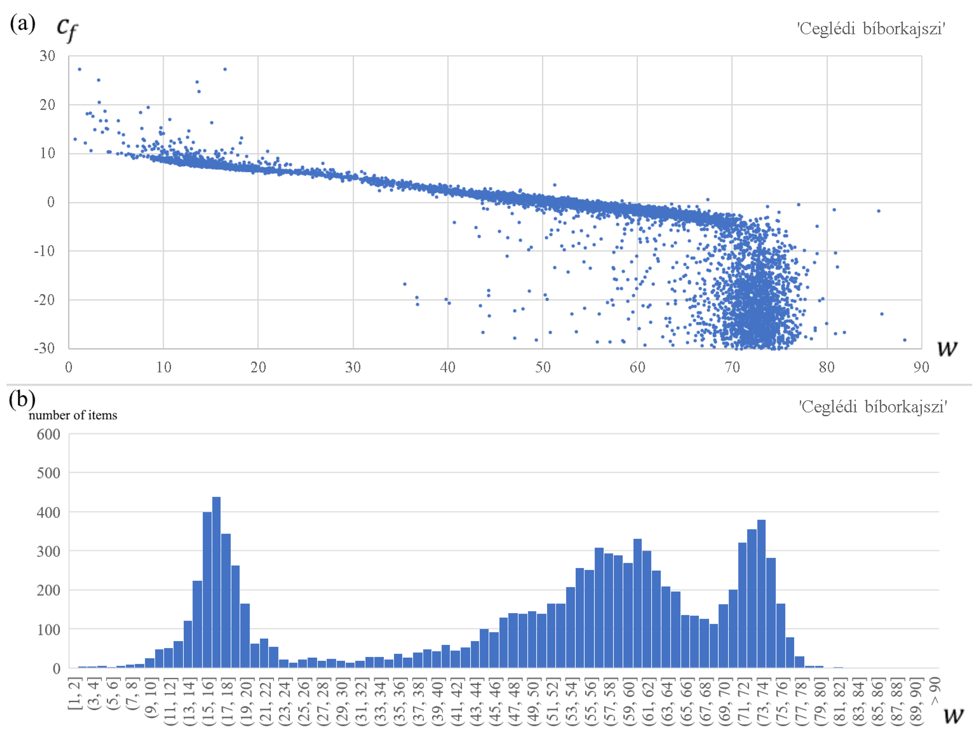
- First, we observe that for each apricot cultivar, the forcing parameters and are strongly related, although not linearly (see the upper panel in Figure 2). Therefore, these two parameters cannot be optimized independently. Using the empirical relationship between and obtained from the optimization process, we calculate the optimal values of for all fixed values of ;
- 2.
- Based on the resulted parameter vectors of all walks, we plot the histogram of the optimal parameter values of (see the lower panel in Figure 2). We see that the optimal parameter values of are dense mainly around three or four small to high values; more exactly, around one small, two medium, and one high value for ‘Rózsakajszi C.1406’, while around one small, one medium, and one high value for the other two cultivars. We immediately exclude the high values, because we obtained values in those cases between −10 °C and −30 °C, which are unlikely during the forcing period in Hungary [9,68];
- 3.
- The results of most walks are dense around the small value for each apricot cultivar, and we obtained the lowest RMSE values here, too. So, we fix the parameter value at the median of the preferred range of ‘small’ optimal parameters : = 15.6, = 17.9, = 19.4;
- 4.
- As a next step, we narrow the parameter space according to the biologically possible parameter values for Hungary (Table 2) [7,9,65,69,70]. In the original parameter space, we find several similarly good parameter vectors, that fit statistically very well to the observed blooming dates, but they are biologically impossible.
- 5.
- Then, we searched for the global optimum of the parameter space for each apricot cultivar. We define the global optimum parameter vector as the parameter vector with the lowest root-mean-square error (RMSE) among the grid of values of Table 4. It is seen that, in many cases (, , , , , , , , , and ), the global optimal parameter values do not fall in the local optimum bins. This is most surprising for the parameter , where more than 70% of the walk limits fall in the local optimal bin, but the global optimum parameter value does not;
- 6.
- Using the global optimum parameter vector, we estimated the blooming date for each apricot cultivar with an average error less than 2.5 days (RMSE < 2.5). For comparison, if we take the mean blooming data calculated over all the years as a constant [64], the average error of the estimation (i.e., the error of the base model) is as high as 9.7–10.6 days, depending on cultivars;
- 7.
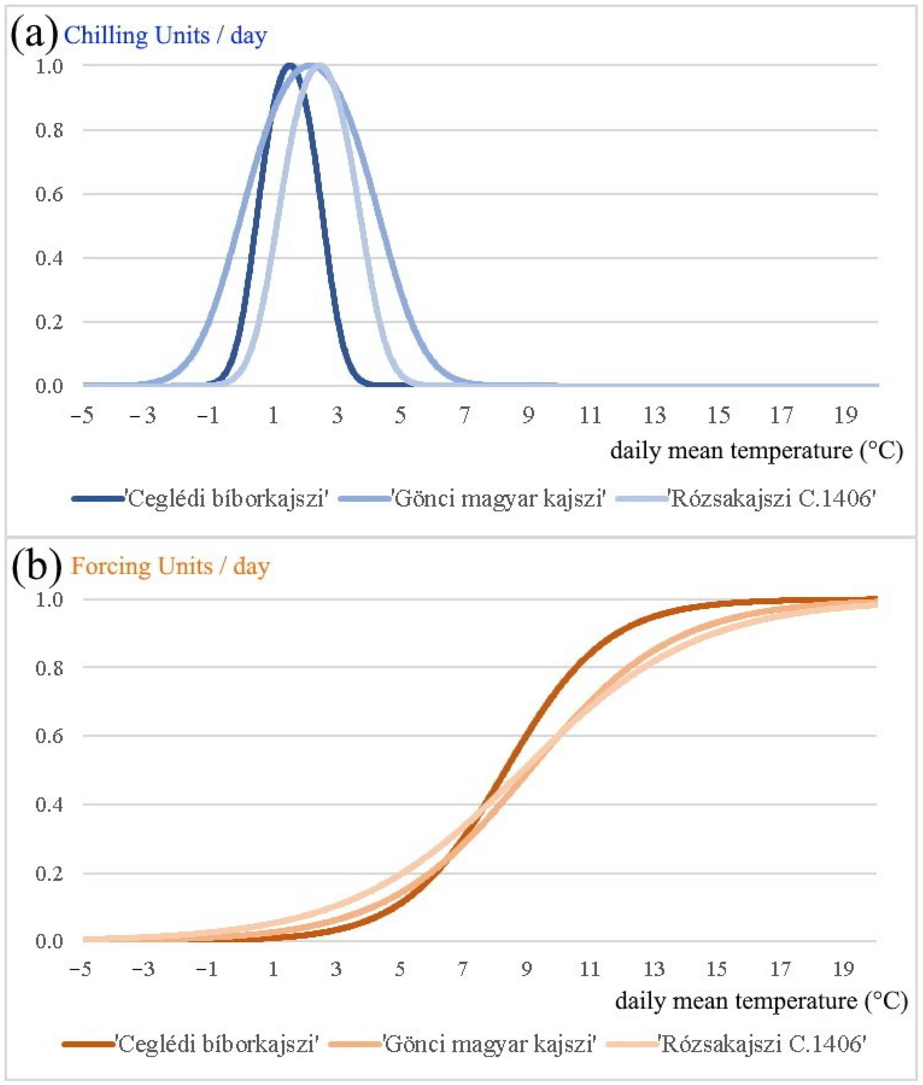
- Finally, based on the daily average temperature and the global optimal parameter vectors, we calculated the critical amount of chilling and forcing units, and determined the chilling and forcing process for each cultivar in the period 1994–2020 (Figure 1 and Figure 3). We provide the parameter values that are optimized with the simulated annealing method, applying the unified model and the observed string stage and blooming data of years 1994–2000 (Table 4). The temperature that is optimal for the plant for chilling unit accumulation () is 1.50 °C for ‘Ceglédi bíborkajszi’, 2.13 °C for ‘Gönci magyar kajszi’, and 2.42 °C for ‘Rózsakajszi C.1406’ in the period 1994–2020. According to our calculations, the most chilling units ( 29.8 units) are necessary for ‘Gönci magyar kajszi’, and the least chilling units ( 12.7 units) are required by ‘Ceglédi bíborkajszi’ for breaking the endodormancy (Table 4). The inflection point of the forcing unit accumulation (i.e., ) is between 8.30 and 9.04 °C, depending on the cultivars. This curve has no maximum point, but the forcing unit accumulation is close to the maximum (1 unit) at 12–15 °C (more than 0.9 units) that could be considered as ‘optimal temperature’ for the plant in their preparation for blooming. The average accumulated forcing units for the blooming are between 14.0 and 16.4 units for each cultivar in the period 1994–2020 (Table 4). Surprisingly, the absolute value of parameter of our results is larger than is reported in the publications of other researchers (i.e., in between −10−4 and −10−8) [8,9,43,64]. This may lead to a conclusion that, in the case of Hungarian apricots, the chilling unit accumulation has a relatively larger effect on forcing unit accumulation.
4. Discussion and Conclusions
Author Contributions
Funding
Institutional Review Board Statement
Data Availability Statement
Conflicts of Interest
References
- Chuine, I.; Kramer, K.; Hänninen, H. Plant development models. In Phenology: An Integrative Environmental Science; Schwartz, M.D., Ed.; Kluwer Academic Publishers: Dordrecht, The Netherlands, 2003; pp. 217–235. [Google Scholar]
- Hänninen, H. Modelling bud dormancy release in trees from cool and temperate regions. Acta For. Fenn. 1990, 213, 7660. [Google Scholar] [CrossRef] [Green Version]
- Williams, D.W.; Andris, H.L.; Beede, R.H.; Luvisi, D.A.; Norton, M.V.K.; Williams, L.E. Validation of a Model for the Growth and Development of the Thompson Seedless Grapevine. II. Phenology. Am. J. Enol. Vitic. 1985, 36, 283–289. [Google Scholar]
- Linkosalo, T.; Carter, T.; Häkkinen, R.; Hari, P. Predicting spring phenology and frost damage risk of Betula spp. Under climatic warming: A comparison of two models. Tree Physiol. 2000, 20, 1175–1182. [Google Scholar] [CrossRef] [Green Version]
- Eccel, E.; Rea, R.; Caffarra, A.; Crisci, A. Risk of spring frost to apple production under future climate scenarios: The role of phenological acclimation. Int. J. Biometeorol. 2009, 53, 273–286. [Google Scholar] [CrossRef]
- Moriondo, M.; Bindi, M. Impact of climate change of typical Mediterranean crops. Ital. J. Agrometorol. 2007, 12, 5–12. [Google Scholar]
- Caffarra, A.; Eccel, E. Increasing the robustness of phenological models for Vitis vinifera cv. Chardonnay. Int. J. Biometeorol. 2010, 54, 255–267. [Google Scholar] [CrossRef] [PubMed]
- Fila, G.; Di Lena, B.; Gardiman, M.; Storchi, P.; Tomasi, D.; Silvestroni, O.; Pitacco, A. Calibration and validation of grapevine budburst models using growth-room experiments as data source. Agric. For. Meteorol. 2012, 160, 69–79. [Google Scholar] [CrossRef]
- Hlaszny, E. A Szőlő (Vitis vinifera L.) Korai Fenológiai Válaszadásának Modellezése a Kunsági Borvidéken Növényfelvételezések, Időjárási Megfigyelések és Regionális Klímamodell Alapján. Ph.D. Thesis, Corvinus University of Budapest, Budapest, Hungary, 2012; 163p. (In Hungarian). [Google Scholar]
- Faust, M.; Erez, A.; Rowland, L.J.; Wang, S.Y.; Norman, H.A. Bud dormancy in perennial fruit trees: Physiological basis for dormancy induction, maintenance, and release. HortScience 1997, 32, 623–629. [Google Scholar] [CrossRef] [Green Version]
- Andreini, L.; García de Cortázar-Atauri, I.; Chuine, I.; Viti, R.; Bartolini, S.; Ruiz, D.; Campoy, J.A.; Legave, J.M.; Audergon Jean-Marc Bertuzzi, P. Understanding dormancy release in apricot flower buds (Prunuus armeniaca L.) using several process-based phenological models. Agric. For. Meteorol. 2014, 184, 210–219. [Google Scholar] [CrossRef]
- Bellini, E. The Fruit Woody Species; ARSIA: Firenze, Italy, 2007; Volume 1–2, 1069p. [Google Scholar]
- Ledbetter, C.A. Apricots. In Temperate Fruit Crop Breeding; Hancock, J.H., Ed.; Springer Science and Business Media B.V.: Dordrecht, The Nederlands, 2008; pp. 39–82. [Google Scholar]
- Campoy, J.A.; Ruiz, D.; Egea, J. Dormancy in temperate fruit trees in a global warming context: A review. Sci. Hortic. 2011, 130, 357–372. [Google Scholar] [CrossRef]
- Soltész, M. Blooming. In Floral Biology of Temperate Zone Fruit Trees and Small Fruits; Nyéki, J., Soltész, M., Eds.; Akadémiai Kiadó: Budapest, Hungary, 1996; pp. 80–131. [Google Scholar]
- Szalay, L. Development and cold hardiness of flower buds of stone fruits. In Morphology, Biology and Fertility of Flowers in Temperate Zone Fruits; Nyéki, J., Soltész, M., Szabó, Z., Eds.; Academic Press: Budapest, Hungary, 2008; pp. 63–82. [Google Scholar]
- Szabó, Z.; Nyéki, J.; Soltész, M. Apricot (Prunus armeniaca L.). In Floral Biology, Pollination and Fertilisation in Temperate Zone Fruit Species and Grape; Kozma, P., Nyéki, J., Soltész, M., Szabó, Z., Eds.; Akadémiai Kiadó: Budapest, Hungary, 2003; pp. 411–423. [Google Scholar]
- Szabó, Z.; Nyéki, J. Blossoming, fructification and combination of apricot varieties. Acta Hortic. 1991, 293, 295–302. [Google Scholar] [CrossRef]
- Pedryc, A. A Kajszibarack Néhány Tulajdonságának Variabilitása a Nemesítés Szemszögéből. Ph.D. Thesis, Hungarian Academy of Sciences, Budapest, Hungary, 1992. (In Hungarian). [Google Scholar]
- Szalay, L.; Szabó, Z. Blooming time of some apricot varieties of different origin in Hungary. Int. J. Hortic. Sci. 1999, 5, 16–20. [Google Scholar] [CrossRef]
- Surányi, D. A Sárgabarack (The Apricot). Magyarország Kultúrflórája II; Kötet, 9, Füzet; Szent István Egyetemi Kiadó: Gödöllő, Hungary, 2011; 303p. (In Hungarian) [Google Scholar]
- Hsiang, T.-F.; Lin, Y.-J.; Yamane, H.; Tao, R. Characterization of Japanese Apricot (Prunus mume) Floral Bud Development Using a Modified BBCH Scale and Analysis of the Relationship between BBCH Stages and Floral Primordium Development and the Dormancy Phase Transition. Horticulturae 2021, 7, 142. [Google Scholar] [CrossRef]
- Della Strada, G.; Pennone, F.; Fideghelli, C.; Monastra, F.; Cobiancchi, D. Monografia di Cultivar di Albicocco; Istituto Sperimentaleper la Frutticoltura: Rome, Italy, 1989; 239p. (In Italian)
- Pirazzini, P. Prove di impollinazione su nueve cultivar di albicocco nell’Imolese. Italus Hortus 1997, 4, 70–71. (In Italian) [Google Scholar]
- Fitter, A.H.; Fitter, R.S.R. Rapid changes in blooming time in British plants. Science 2002, 296, 1689–1691. [Google Scholar] [CrossRef]
- Parmesan, C.; Yohe, G. A globally coherent fingerprint of climate change impacts across natural systems. Nature 2003, 421, 37–42. [Google Scholar] [CrossRef] [PubMed]
- Chmielewski, F.-M.; Müller, A.; Bruns, E. Climate changes and trends in phenology of fruit trees and field crops in Germany, 1961–2000. Agric. For. Meteorol. 2004, 121, 69–78. [Google Scholar] [CrossRef]
- Wolfe, D.W.; Schwartz, M.D.; Lakso, A.N.; Otsuki, Y.; Pool, R.M.; Shaulis, N.J. Climate change and shifts in spring phenology of three horticultural woody perennials in north eastern USA. Int. J. Biometeorol. 2005, 49, 303–309. [Google Scholar] [CrossRef] [PubMed]
- Legave, J.M.; Clauzel, G. Long-term evolution of flowering time in apricot cultivars grown in southern France: Which future impacts of global warming? Acta Hortic. 2006, 717, 47–50. [Google Scholar] [CrossRef]
- Parmesan, C. Influences of species, latitudes and methodologies on estimates of phenological response to global warming. Glob. Change Biol. 2007, 13, 1860–1872. [Google Scholar] [CrossRef]
- Legave, J.M.; Christen, D.; Giovannini, D.; Oger, R. Global warming in Europe and its impact on floral bud phenology in fruit species. Acta Hortic. 2009, 838, 21–26. [Google Scholar] [CrossRef]
- Grab, S.; Craparo, A. Advance of apple and pear tree full bloom dates in response to climate change in the south western Cape, South Africa: 1973–2009. Agric. For. Meteorol. 2011, 151, 406–413. [Google Scholar] [CrossRef]
- Cook, B.I.; Wolkovich, E.M.; Parmesan, C. Divergent responses to spring and winter warming drive community level blooming trends. Proc. Natl. Acad. Sci. USA 2012, 109, 9000–9005. [Google Scholar] [CrossRef] [PubMed] [Green Version]
- Szalay, L.; Froemel-Hajnal, V.; Bakos, J.; Ladányi, M. Changes of the microsporogenesis process and blooming time of three apricot genotypes (Prunus armeniaca L.) in Central Hungary based on long-term observation (1994–2018). Sci. Hortic. 2019, 246, 279–288. [Google Scholar] [CrossRef]
- Yu, H.; Luedeling, E.; Xu, J. Winter and spring warming result in delayed spring phenology on the Tibetan Plateau. Proc. Natl. Acad. Sci. USA 2010, 107, 22151–22156. [Google Scholar] [CrossRef] [PubMed] [Green Version]
- Bartolini, S.; Massani, R.; Iacona, C.; Guerriero, R.; Viti, R. Forty-year investigations on apricot blooming: Evidences of climate change effects. Sci. Hortic. 2019, 244, 399–405. [Google Scholar] [CrossRef]
- Bartolini, S.; Massai, R.; Viti, R. The influence of autumn-winter temperatures on endodormancy release and blooming performance of apricot (Prunus armeniaca L.) in central Italy based on long-term observations. J. Hortic. Sci. Biotechnol. 2020, 95, 794–803. [Google Scholar] [CrossRef]
- Guo, L.; Dai, J.; Wang, M.; Xu, J.; Luedeling, E. Responses of spring phenology in temperate zone trees to climate warming: A case study of apricot blooming in China. Agric. For. Meteorol. 2015, 201, 1–7. [Google Scholar] [CrossRef] [Green Version]
- Luedeling, E. Climate change impacts on winter chill for temperate fruit and nut production: A review. Sci. Hortic. 2012, 144, 218–229. [Google Scholar] [CrossRef] [Green Version]
- Campoy, J.A.; Audergon, J.M.; Ruiz, D. Genomic designing for new climate-resilient apricot varieties in a warming context. In Genomic Designing of Climate-Smart Fruit Crops; Kole, C., Ed.; Springer Nature: Cham, Switzerland, 2020; pp. 73–90. [Google Scholar]
- Rodrigo, J.; Herrero, M. Effects of pre-blossom temperatures on flower development and fruit set in apricot. Sci. Hortic. 2002, 92, 125–135. [Google Scholar] [CrossRef] [Green Version]
- Lakatos, L.; Nyéki, J.; Soltész, M.; Szabó, Z.; Racskó, J. Effect of meteorological variables on the blooming time. In Morphology, Biology and Fertility of Flowers in Temperate Zone Fruits; Nyéki, J., Soltész, M., Szabó, Z., Eds.; Akadémiai Kiadó: Budapest, Hungary, 2008; pp. 117–140. [Google Scholar]
- Chuine, I. A Unified Model for Budburst of Trees. J. Theor. Biol. 2000, 207, 337–347. [Google Scholar] [CrossRef] [PubMed]
- Fu, Y.H.; Campioli, M.; Demarée, G.; Deckmyn, A.; Hamdi, R.; Janssens, I.A.; Deckmyn, G. Bayesian calibration of the Unified budburst model in six temperate tree species. Int. J. Biometeorol. 2012, 56, 153–164. [Google Scholar] [CrossRef] [PubMed]
- Richardson, E.A.; Seeley, S.D.; Walker, D.R. A model for estimating the completion of rest for ‘Redhaven’ and ‘Elberta’ peach trees. HortScience 1974, 9, 331–332. [Google Scholar]
- Sarvas, R. Investigations on the Annual Cycle of Development of Forest Trees: Autumn Dormancy and Winter Dormancy; Communicationes Instituti Forestalis Fenniae: Vantaa, Finland, 1974; Volume 84, pp. 1–101. [Google Scholar]
- Hänninen, H. Effects of temperature on dormancy release in woody plants: Implications of prevailing models. Silva Fenn. 1987, 21, 279–299. [Google Scholar] [CrossRef] [Green Version]
- Landsberg, J.J. Apple fruit bud development and growth; analysis and an empirical model. Ann. Bot. 1974, 38, 1013–1023. [Google Scholar] [CrossRef]
- Kobayashi, K.D.; Fuchigami, L.H.; English, M.J. Modelling temperature requirements for rest development in Cornus sericea. J. Am. Soc. Horic. Sci. 1982, 107, 914–918. [Google Scholar]
- Vegis, A. Dormancy in higher plants. Annu. Rev. Plant Physiol. 1964, 15, 185–224. [Google Scholar] [CrossRef]
- Press, W.H.; Teukoisky, S.A.; Vetterling, W.T.; Flannery, B.P. The Art of Scientific Computing. In Numerical Recipes, 3rd ed.; Cambridge University Press: Cambridge, UK, 2007; 1235p. [Google Scholar]
- Weise, T. Global Optimization Algorithms–Theory and Application, 2nd ed.; e-book; Thomas Weise’s private publication; 2009; pp. 263–267. Available online: http://www.it-weise.de/projects/book.pdf (accessed on 11 July 2022).
- Chuine, I.; Cour, P.; Rousseau, D.D. Fitting models predicting dates of blooming of temperate-zone trees using simulated annealing. Plant Cell Environ. 1998, 21, 455–466. [Google Scholar] [CrossRef]
- WMO. Volume I—Measurement of Meteorological Variables, No. 8. In Guide to Instruments and Methods of Observation; World Meteorological Organization: Geneva, Switzerland, 2018; p. 548. [Google Scholar]
- Legave, J.M.; Blanke, M.; Christen, D.; Giovannini, D.; Mathieu, V.; Oger, R. A comprehensive overview of spatial and temporal variability of apple bud dormancy release and blooming phenology in Western Europe. Int. J. Biometeorol. 2013, 57, 317–331. [Google Scholar] [CrossRef]
- Guo, L.; Dai, J.; Ranjitkar, S.; Yu, H.; Xu, J.; Luedeling, E. Chilling and heat requirements for blooming in temperate fruit trees. Int. J. Biometeorol. 2014, 58, 1195–1206. [Google Scholar] [CrossRef]
- Cannell, M.G.R.; Smith, R.I. Thermal Time, chill days and prediction of budburst in Picea sitchensis. J. Appl. Ecol. 1983, 20, 951–963. [Google Scholar] [CrossRef]
- Murray, M.B.; Cannell, G.R.; Smith, R.I. Date of budburst of fit teen tree species in Britain following climate warming. J. Appl. Ecol. 1989, 26, 693–700. [Google Scholar] [CrossRef]
- Heide, O. Dormancy release in beech buds (Fagus sylvatica) requires both chilling and long days. Physiol. Plant 1993, 89, 187–191. [Google Scholar] [CrossRef]
- Myking, T.; Heide, O.M. Dormancy release and chilling requirement of buds of latitudinal ecotypes of Betula pendula and B. pubescens. Tree Physiol. 1995, 15, 697–704. [Google Scholar] [CrossRef]
- Chuine, I.; Cour, P. Climatic determinants of budburst seasonality of temperate-zone trees. New Phytol. 1999, 143, 339–349. [Google Scholar] [CrossRef]
- Janssen, P.H.M.; Heuberger, P.S.C. Calibration of process-oriented models. Ecol. Model. 1995, 83, 55–66. [Google Scholar] [CrossRef]
- Fan, D.; Zhu, W.; Zheng, Z.; Zhang, D.; Pan, Y.; Jiang, N. Change in the Green-Up Dates for Quercus mongolica in Northeast China and Its Climate-Driven Mechanism from 1962 to 2012. PLoS ONE 2015, 10, e0130516. [Google Scholar] [CrossRef] [Green Version]
- Dai, W.; Jin, H.; Zhang, Y.; Liu, T.; Zhou, Z. Detecting temporal changes in the temperature sensitivity of spring phenology with global warming: Application of machine learning in phenological model. Agric. For. Meteorol. 2019, 279, 14. [Google Scholar] [CrossRef]
- Thornley, J.H.M.; Johnson, R. Plant and Crop Modelling: A Mathematical Approach to Plant and Crop Physiology; Clarendon Press: Oxford, UK, 1990; 684p. [Google Scholar]
- Németh, S. A Virágrügy- és Gyümölcsfejlődés Fenológiai, Morfológiai és Biokémiai Jellemzése Fontosabb Kajszifajták Esetében. Ph.D. Thesis, Corvinus University of Budapest, Budapest, Hungary, 2012; 146p. (In Hungarian). [Google Scholar]
- Herrera, S.; Lora, J.; Fadón, E.; Hedhly, A.; Alonso, J.M.; Hormaza, J.I.; Rodrigo, J. Male Meiosis as a Biomarker for Endo- to Ecodormancy Transition in Apricot. Front. Plant Sci. 2022, 13, 842333. [Google Scholar] [CrossRef]
- Chuine, I.; Bonhomme, M.; Legave, J.-M.; García de Cortázar-Atauri, I.; Charrier, G.; Lacointe, A.; Améglio, T. 2016: Can phenological models predict tree phenology accurately in the future? The unrevealed hurdle of endodormancy break. Glob. Change Biol. 2016, 22, 3444–3460. [Google Scholar] [CrossRef]
- Campoy, J.A.; Ruiz, D.; Nortes, M.D.; Egea, J. Temperature efficiency for dormancy release in apricot varies when applied at different amounts of chilling accumulation. Plant Biol. 2012, 15, 28–35. [Google Scholar] [CrossRef] [PubMed]
- Gao, Z.; Zhuang, W.; Wang, L.; Shao, J.; Luo, X.; Cai, B.; Zhang, Z. Evaluation of Chilling and Heat Requirements in Japanese Apricot with Three Models. HortScience 2012, 47, 1826–1831. [Google Scholar] [CrossRef] [Green Version]
- Bartholy, J.; Pongrácz, R. Klímaváltozás; Lecture Notes; Eötvös Loránd University: Budapest, Hungary, 2013; 180p. (In Hungarian) [Google Scholar]
- Viti, R.; Monteleone, P. Observations on flower bud growth in some low yield varieties of apricot. Acta Hortic. 1991, 293, 319–326. [Google Scholar] [CrossRef]
- Sunley, R.J.; Atkinson, C.J.; Jones, H.G. Chill unit models and recent changes in the occurrence of winter chill and spring frost in the United Kingdom. J. Hortic. Sci. Biotechnol. 2006, 81, 949–958. [Google Scholar] [CrossRef]
- Legave, J.; Farrera, I.; Alméras, T.; Calleja, M. Selecting models of apple flowering time and understanding how global warming has had an impact on this trait. J. Hortic. Sci. Biotechnol. 2008, 83, 76–84. [Google Scholar] [CrossRef]
- Garcia de Cortazar-Atauri, I.; Brisson, N.; Gaudillere, J. Performance of several models for predicting budburst date of grapevine (Vitis vinifera L.). Int. J. Biometeorol. 2009, 53, 317–326. [Google Scholar] [CrossRef]
- Chuine, I. Why does phenology drive species distribution? Philos. Trans. Biol. Sci. 2010, 365, 3149–3160. [Google Scholar] [CrossRef] [Green Version]
- Vitasse, Y.; Francois, C.; Delpierre, N.; Dufrene, E.; Kremer, A.; Chuine, I.; Delzon, S. Assessing the effects of climate change on the phenology of European temperate trees. Agric. For. Meteorol. 2011, 151, 969–980. [Google Scholar] [CrossRef]
- Chmielewski, F.-M.; Blümel, K.; Henniges, Y.; Blanke, M.; Weber, R.W.S.; Zoth, M. Phenological models for the beginning of apple blossom in Germany. Meteorol. Z. 2011, 20, 487–496. [Google Scholar] [CrossRef]
- Pouget, R. Méthode d’appréciation de l’évolution physiologique des bourgeons pendant la phase de pré-débourrement. Application à l’étude comparée du débourrement de la vigne. Vitis 1967, 6, 294–302. (In French) [Google Scholar]
- Hauagge, R.; Cummins, J. Pome Fruit Genetic Pool for Production in Warm Climates. In Temperate Fruit Crops in Warm Climates; Erez, A., Ed.; Springer: Amsterdam, The Netherlands, 2000; pp. 267–303. [Google Scholar]
- Vitasse, Y.; Hoch, G.; Randin, C.F.; Lenz, A.; Kollas, C.; Scheepens, J.F.; Körner, C. Elevational adaptation and plasticity in seedling phenology of temperate deciduous tree species. Oecologia 2013, 171, 663–678. [Google Scholar] [CrossRef]
- Pór, J. Kajsziültetvények létesítése. In Kajszi; Pénzes, B., Szalay, L., Eds.; Mezőgazda Kiadó: Budapest, Hungary, 2003; pp. 186–197. (In Hungarian) [Google Scholar]
- Hufkens, K.; Basler, D.; Milliman, T.; Melaas, E.K.; Richardson, A.D. An integrated phenology modelling framework in R. Methods Ecol. Evol. 2018, 9, 1276–1285. [Google Scholar] [CrossRef] [Green Version]
- Atagul, O.; Calle, A.; Demirel, G.; Lawton, J.N.; Bridges, W.C.; Gasic, K. Estimating Heat Requirement for Flowering in Peach Germplasm. Agronomy 2022, 12, 1002. [Google Scholar] [CrossRef]
- Eduardo Fernandez, E.; Krefting, P.; Kunz, A.; Do, H.; Fadón, E.; Luedeling, E. Boosting statistical delineation of chill and heat periods in temperate fruit trees through multi-environment observations. Agric. For. Meteorol. 2021, 310, 108652. [Google Scholar] [CrossRef]
- Yang, J.; Huo, Z.; Wang, P.; Wu, D.; Ma, Y.; Yao, S.; Dong, H. Process-based indicators for timely identification of apricot frost disaster on the warm temperate zone, China. Theor. Appl. Climatol. 2021, 146, 1143–1155. [Google Scholar] [CrossRef]


| Parameter | Minimum Value | Maximum Value | Step Length |
|---|---|---|---|
| 0 | 10 | 0.01 | |
| −50 | 50 | 0.10 | |
| −10 | 0 | 0.01 | |
| −30 | 30 | 0.10 | |
| 0 | 200 | 0.10 | |
| 2 | 9 | 0.01 |
| Parameter | Minimum Value | Maximum Value | Step Length |
|---|---|---|---|
| 0.2 | 1.0 | 0.001 | |
| 1 | 5 | 0.005 | |
| −0.9 | −0.1 | 0.001 | |
| 6 | 14 | 0.010 | |
| 2 | 6 | 0.005 |
| Minimum | 0.568 | 1.400 | −0.436 | 7.600 | 2.080 | 0.248 | 3.160 | −0.420 | 7.280 | 2.040 | 0.312 | 2.640 | −0.556 | 7.360 | 2.040 |
| Maximum | 0.576 | 1.440 | −0.428 | 9.280 | 2.480 | 0.256 | 3.200 | −0.380 | 9.040 | 2.400 | 0.320 | 2.720 | −0.484 | 8.560 | 2.600 |
| No. of items | 128 | 129 | 156 | 7480 | 1592 | 143 | 138 | 735 | 7950 | 1680 | 132 | 270 | 1318 | 7180 | 2210 |
| Median | 0.572 | 1.420 | −0.432 | 8.210 | 2.260 | 0.252 | 3.180 | −0.400 | 7.880 | 2.220 | 0.316 | 2.680 | −0.520 | 7.710 | 2.310 |
| St. deviation | 0.002 | 0.010 | 0.002 | 0.420 | 0.110 | 0.002 | 0.010 | 0.011 | 0.430 | 0.100 | 0.002 | 0.020 | 0.021 | 0.310 | 0.160 |
| Maximum RMSE | 4.40 | 4.17 | 3.40 | 4.60 | 4.39 | 5.04 | 4.66 | 4.58 | 7.18 | 4.68 | 4.78 | 5.63 | 4.62 | 5.78 | 5.05 |
| Median RMSE | 2.92 | 2.94 | 2.84 | 2.86 | 2.66 | 2.82 | 2.81 | 2.79 | 2.81 | 2.49 | 2.47 | 2.38 | 2.41 | 2.41 | 2.15 |
| St. dev. RMSE | 0.33 | 0.33 | 0.18 | 0.21 | 0.31 | 0.49 | 0.43 | 0.27 | 0.25 | 0.33 | 0.57 | 0.63 | 0.31 | 0.31 | 0.50 |
| Parameter | ‘Ceglédi bíborkajszi’ | ‘Gönci magyar kajszi’ | ‘Rózsakajszi C.1406’ |
|---|---|---|---|
| 0.949 | 0.216 | 0.608 | |
| 1.50 | 2.13 | 2.42 | |
| −0.626 | −0.443 | −0.365 | |
| 8.30 | 9.04 | 8.84 | |
| 15.60 | 17.90 | 19.40 | |
| 2.14 (−0.0072) | 2.08 (−0.0083) | 2.07 (−0.0086) | |
| 14th of January | 22nd of January | 30th of January | |
| 27th of March | 29th of March | 1st of April | |
| 12.73 | 29.78 | 19.69 | |
| 14.24 | 13.99 | 16.41 | |
| 14.57 | 14.31 | 16.82 | |
| RMSE | 2.37 | 2.10 | 1.49 |
| Observed BM | Estimated BM | |||||
|---|---|---|---|---|---|---|
| Ceglédi bíborkajszi | Mean | 207.9 | 208.4 | 14.2 | 12.7 | 14.6 |
| StDev | 10.8 | 12.1 | 0.4 | 3.8 | 0.5 | |
| Range | 48.0 | 51.0 | 1.5 | 14.8 | 1.7 | |
| LCI | 203.8 | 203.7 | 14.1 | 11.3 | 14.4 | |
| UCI | 212.1 | 213.1 | 14.4 | 14.2 | 14.7 | |
| Slope | −0.224 | −0.219 | 0.004 | −0.041 | −0.001 | |
| p | 0.438 | 0.500 | 0.696 | 0.686 | 0.933 | |
| Gönci magyar kajszi | Mean | 210.3 | 210.2 | 14.0 | 29.8 | 14.3 |
| StDev | 10.6 | 11.2 | 0.8 | 6.5 | 0.8 | |
| Range | 46.0 | 47.0 | 2.6 | 22.3 | 2.8 | |
| LCI | 206.2 | 205.9 | 13.7 | 27.3 | 14.0 | |
| UCI | 214.3 | 214.5 | 14.3 | 32.3 | 14.6 | |
| Slope | −0.283 | −0.213 | 0.001 | −0.005 | −0.003 | |
| p | 0.316 | 0.479 | 0.978 | 0.977 | 0.881 | |
| Rózsakajszi C.1406 | Mean | 212.9 | 212.8 | 16.4 | 19.7 | 16.8 |
| StDev | 10.0 | 10.2 | 0.7 | 4.7 | 0.7 | |
| Range | 41.0 | 40.0 | 2.6 | 18.9 | 3.2 | |
| LCI | 209.0 | 208.9 | 16.2 | 17.9 | 16.5 | |
| UCI | 216.7 | 216.7 | 16.7 | 21.5 | 17.1 | |
| Slope | −0.305 | −0.257 | −0.001 | 0.012 | 0.003 | |
| p | 0.252 | 0.344 | 0.933 | 0.925 | 0.880 |
Publisher’s Note: MDPI stays neutral with regard to jurisdictional claims in published maps and institutional affiliations. |
© 2022 by the authors. Licensee MDPI, Basel, Switzerland. This article is an open access article distributed under the terms and conditions of the Creative Commons Attribution (CC BY) license (https://creativecommons.org/licenses/by/4.0/).
Share and Cite
Mesterházy, I.; Raffai, P.; Szalay, L.; Bozó, L.; Ladányi, M. Estimation of Blooming Start with the Adaptation of the Unified Model for Three Apricot Cultivars (Prunus armeniaca L.) Based on Long-Term Observations in Hungary (1994–2020). Diversity 2022, 14, 560. https://doi.org/10.3390/d14070560
Mesterházy I, Raffai P, Szalay L, Bozó L, Ladányi M. Estimation of Blooming Start with the Adaptation of the Unified Model for Three Apricot Cultivars (Prunus armeniaca L.) Based on Long-Term Observations in Hungary (1994–2020). Diversity. 2022; 14(7):560. https://doi.org/10.3390/d14070560
Chicago/Turabian StyleMesterházy, Ildikó, Péter Raffai, László Szalay, László Bozó, and Márta Ladányi. 2022. "Estimation of Blooming Start with the Adaptation of the Unified Model for Three Apricot Cultivars (Prunus armeniaca L.) Based on Long-Term Observations in Hungary (1994–2020)" Diversity 14, no. 7: 560. https://doi.org/10.3390/d14070560