
Propensity Score Analysis with Partially Observed Baseline Covariates: A Practical Comparison of Methods for Handling Missing Data

 , , ,
, , ,  and
and 
Abstract
:1. Introduction
1.1. Motivating Example
1.2. Propensity Score Framework
2. Materials and Methods
2.1. Propensity Score and Missing Data in Non-Interventional Studies
2.2. Statistical Analysis
2.2.1. Propensity Score Estimation
2.2.2. Missing Data Methods
2.2.3. Measures of Balance
3. Results
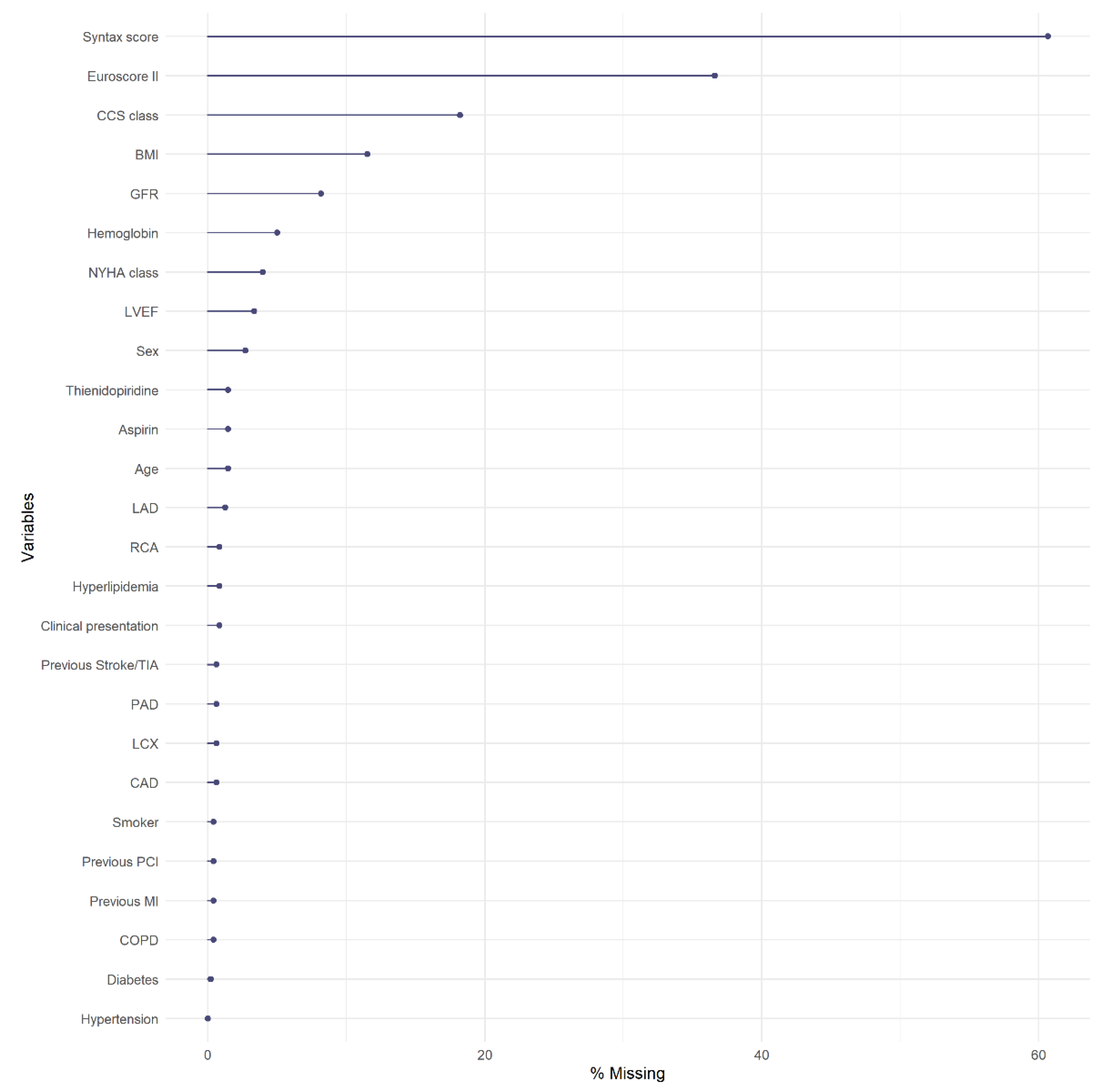
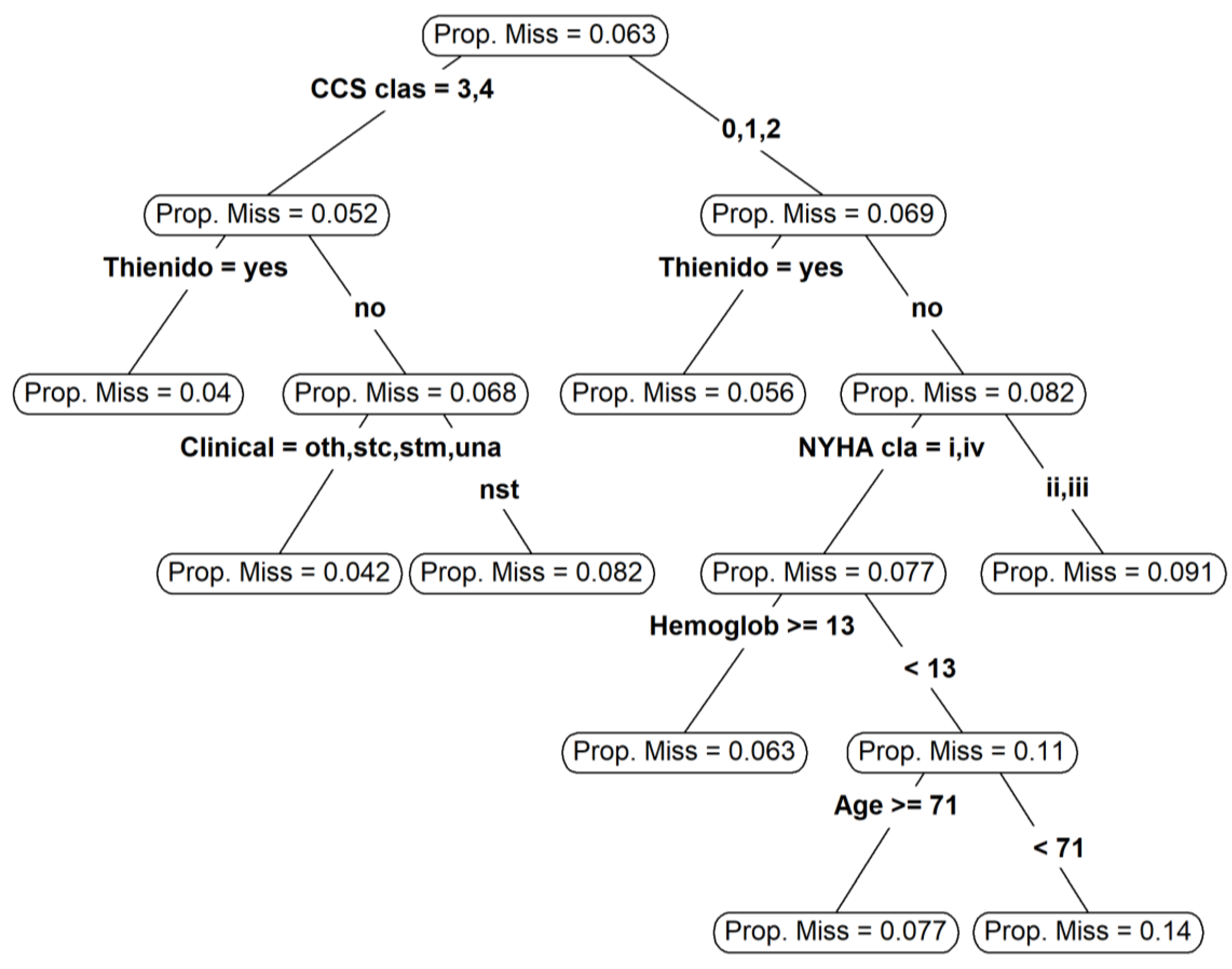
3.1. Missing Data
3.2. Propensity Score Estimation and Common Support
3.3. Balance
4. Discussion
5. Conclusions
Author Contributions
Funding
Institutional Review Board Statement
Informed Consent Statement
Data Availability Statement
Acknowledgments
Conflicts of Interest
References
- Austin, P.C. An Introduction to Propensity Score Methods for Reducing the Effects of Confounding in Observational Studies. Multivar. Behav. Res. 2011, 46, 399–424. [Google Scholar] [CrossRef] [Green Version]
- Rubin, D.B. For Objective Causal Inference, Design Trumps Analysis. Ann. Appl. Stat. 2008, 2, 808–840. [Google Scholar] [CrossRef]
- Rosenbaum, P.R.; Rubin, D.B. The Central Role of the Propensity Score in Observational Studies for Causal Effects. Biometrika 1983, 70, 41–55. [Google Scholar] [CrossRef]
- Elze, M.C.; Gregson, J.; Baber, U.; Williamson, E.; Sartori, S.; Mehran, R.; Nichols, M.; Stone, G.W.; Pocock, S.J. Comparison of Propensity Score Methods and Covariate Adjustment: Evaluation in 4 Cardiovascular Studies. J. Am. Coll. Cardiol. 2017, 69, 345–357. [Google Scholar] [CrossRef]
- Benedetto, U.; Head, S.J.; Angelini, G.D.; Blackstone, E.H. Statistical Primer: Propensity Score Matching and Its Alternatives. Eur. J. Cardiothorac. Surg. 2018, 53, 1112–1117. [Google Scholar] [CrossRef] [Green Version]
- Ellis, A.G.; Trikalinos, T.A.; Wessler, B.S.; Wong, J.B.; Dahabreh, I.J. Propensity Score-Based Methods in Comparative Effectiveness Research on Coronary Artery Disease. Am. J. Epidemiol. 2018, 187, 1064–1078. [Google Scholar] [CrossRef]
- McMurry, T.L.; Hu, Y.; Blackstone, E.H.; Kozower, B.D. Propensity Scores: Methods, Considerations, and Applications in the Journal of Thoracic and Cardiovascular Surgery. J. Thorac. Cardiovasc. Surg. 2015, 150, 14–19. [Google Scholar] [CrossRef] [Green Version]
- Bangalore, S.; Guo, Y.; Samadashvili, Z.; Blecker, S.; Xu, J.; Hannan, E.L. Everolimus-Eluting Stents or Bypass Surgery for Multivessel Coronary Disease. N. Engl. J. Med. 2015, 372, 1213–1222. [Google Scholar] [CrossRef] [Green Version]
- Rosenbaum, P.R. Model-Based Direct Adjustment. J. Am. Stat. Assoc. 1987, 82, 387–394. [Google Scholar] [CrossRef]
- Austin, P.C.; Stuart, E.A. Optimal Full Matching for Survival Outcomes: A Method That Merits More Widespread Use. Stat. Med. 2015, 34, 3949–3967. [Google Scholar] [CrossRef]
- Austin, P.C.; Stuart, E.A. Estimating the Effect of Treatment on Binary Outcomes Using Full Matching on the Propensity Score. Stat. Methods Med. Res. 2017, 26, 2505–2525. [Google Scholar] [CrossRef]
- White, I.R.; Carlin, J.B. Bias and Efficiency of Multiple Imputation Compared with Complete-Case Analysis for Missing Covariate Values. Stat. Med. 2010, 29, 2920–2931. [Google Scholar] [CrossRef]
- Rosenbaum, P.R.; Rubin, D.B. Reducing Bias in Observational Studies Using Subclassification on the Propensity Score. J. Am. Stat. Assoc. 1984, 79, 516–524. [Google Scholar] [CrossRef]
- Rubin, D.B. Multiple Imputation for Nonresponse in Surveys; Wiley: Hoboken, NJ, USA, 1987; ISBN 978-0-471-08705-2. [Google Scholar]
- Friedman, J.H. Greedy Function Approximation: A Gradient Boosting Machine. Ann. Statist. 2001, 29, 1189–1232. [Google Scholar] [CrossRef]
- Choi, B.Y.; Gelfond, J. The Validity of Propensity Score Analysis Using Complete Cases with Partially Observed Covariates. Eur. J. Epidemiol. 2020, 35, 87–88. [Google Scholar] [CrossRef]
- Cham, H.; West, S.G. Propensity Score Analysis with Missing Data. Psychol. Methods 2016, 21, 427–445. [Google Scholar] [CrossRef]
- Coffman, D.L.; Zhou, J.; Cai, X. Comparison of Methods for Handling Covariate Missingness in Propensity Score Estimation with a Binary Exposure. BMC Med Res. Methodol. 2020, 20, 168. [Google Scholar] [CrossRef]
- Stone, G.W.; Sabik, J.F.; Serruys, P.W.; Simonton, C.A.; Généreux, P.; Puskas, J.; Kandzari, D.E.; Morice, M.-C.; Lembo, N.; Brown, W.M.; et al. Everolimus-Eluting Stents or Bypass Surgery for Left Main Coronary Artery Disease. N. Engl. J. Med. 2016, 375, 2223–2235. [Google Scholar] [CrossRef]
- Mäkikallio, T.; Holm, N.R.; Lindsay, M.; Spence, M.S.; Erglis, A.; Menown, I.B.A.; Trovik, T.; Eskola, M.; Romppanen, H.; Kellerth, T.; et al. Percutaneous Coronary Angioplasty versus Coronary Artery Bypass Grafting in Treatment of Unprotected Left Main Stenosis (NOBLE): A Prospective, Randomised, Open-Label, Non-Inferiority Trial. Lancet 2016, 388, 2743–2752. [Google Scholar] [CrossRef] [Green Version]
- Choi, K.H.; Song, Y.B.; Lee, J.M.; Lee, S.Y.; Park, T.K.; Yang, J.H.; Choi, J.-H.; Choi, S.-H.; Gwon, H.-C.; Hahn, J.-Y. Impact of Intravascular Ultrasound-Guided Percutaneous Coronary Intervention on Long-Term Clinical Outcomes in Patients Undergoing Complex Procedures. JACC Cardiovasc. Interv. 2019, 12, 607–620. [Google Scholar] [CrossRef] [PubMed]
- Jones, D.A.; Rathod, K.S.; Koganti, S.; Hamshere, S.; Astroulakis, Z.; Lim, P.; Sirker, A.; O’Mahony, C.; Jain, A.K.; Knight, C.J.; et al. Angiography Alone Versus Angiography Plus Optical Coherence Tomography to Guide Percutaneous Coronary Intervention: Outcomes From the Pan-London PCI Cohort. JACC Cardiovasc. Interv. 2018, 11, 1313–1321. [Google Scholar] [CrossRef]
- Ali, Z.A.; Maehara, A.; Généreux, P.; Shlofmitz, R.A.; Fabbiocchi, F.; Nazif, T.M.; Guagliumi, G.; Meraj, P.M.; Alfonso, F.; Samady, H.; et al. Optical Coherence Tomography Compared with Intravascular Ultrasound and with Angiography to Guide Coronary Stent Implantation (ILUMIEN III: OPTIMIZE PCI): A Randomised Controlled Trial. Lancet 2016, 388, 2618–2628. [Google Scholar] [CrossRef]
- Harris, P.A.; Taylor, R.; Minor, B.L.; Elliott, V.; Fernandez, M.; O’Neal, L.; McLeod, L.; Delacqua, G.; Delacqua, F.; Kirby, J.; et al. The REDCap Consortium: Building an International Community of Software Platform Partners. J. Biomed. Inform. 2019, 95, 103208. [Google Scholar] [CrossRef]
- Harris, P.A.; Taylor, R.; Thielke, R.; Payne, J.; Gonzalez, N.; Conde, J.G. Research Electronic Data Capture (REDCap)—A Metadata-Driven Methodology and Workflow Process for Providing Translational Research Informatics Support. J. Biomed. Inform. 2009, 42, 377–381. [Google Scholar] [CrossRef] [Green Version]
- Westreich, D.; Lessler, J.; Funk, M.J. Propensity Score Estimation: Neural Networks, Support Vector Machines, Decision Trees (CART), and Meta-Classifiers as Alternatives to Logistic Regression. J. Clin. Epidemiol. 2010, 63, 826–833. [Google Scholar] [CrossRef] [Green Version]
- McCaffrey, D.F.; Griffin, B.A.; Almirall, D.; Slaughter, M.E.; Ramchand, R.; Burgette, L.F. A Tutorial on Propensity Score Estimation for Multiple Treatments Using Generalized Boosted Models. Stat. Med. 2013, 32, 3388–3414. [Google Scholar] [CrossRef] [Green Version]
- Imai, K.; Ratkovic, M. Covariate Balancing Propensity Score. J. R. Stat. Soc. 2014, 76, 243–263. [Google Scholar] [CrossRef]
- Cangul, M.Z.; Chretien, Y.R.; Gutman, R.; Rubin, D.B. Testing Treatment Effects in Unconfounded Studies under Model Misspecification: Logistic Regression, Discretization, and Their Combination. Stat. Med. 2009, 28, 2531–2551. [Google Scholar] [CrossRef]
- Gutman, R.; Rubin, D.B. Robust Estimation of Causal Effects of Binary Treatments in Unconfounded Studies with Dichotomous Outcomes. Stat. Med. 2013, 32, 1795–1814. [Google Scholar] [CrossRef]
- Gutman, R.; Rubin, D.B. Estimation of Causal Effects of Binary Treatments in Unconfounded Studies with One Continuous Covariate. Stat. Methods Med Res. 2015. [Google Scholar] [CrossRef] [Green Version]
- Hansen, B.B. Full Matching in an Observational Study of Coaching for the SAT. J. Am. Stat. Assoc. 2004, 99, 609–618. [Google Scholar] [CrossRef] [Green Version]
- Austin, P.C.; Stuart, E.A. The Effect of a Constraint on the Maximum Number of Controls Matched to Each Treated Subject on the Performance of Full Matching on the Propensity Score When Estimating Risk Differences. Stat. Med. 2021, 40, 101–118. [Google Scholar] [CrossRef] [PubMed]
- Jakobsen, J.C.; Gluud, C.; Wetterslev, J.; Winkel, P. When and How Should Multiple Imputation Be Used for Handling Missing Data in Randomised Clinical Trials–A Practical Guide with Flowcharts. BMC Med Res. Methodol. 2017, 17, 162. [Google Scholar] [CrossRef] [PubMed] [Green Version]
- Blake, H.A.; Leyrat, C.; Mansfield, K.E.; Seaman, S.; Tomlinson, L.A.; Carpenter, J.; Williamson, E.J. Propensity Scores Using Missingness Pattern Information: A Practical Guide. Stat. Med. 2020, 39, 1641–1657. [Google Scholar] [CrossRef] [Green Version]
- Groenwold, R.H.H.; White, I.R.; Donders, A.R.T.; Carpenter, J.R.; Altman, D.G.; Moons, K.G.M. Missing Covariate Data in Clinical Research: When and When Not to Use the Missing-Indicator Method for Analysis. CMAJ 2012, 184, 1265–1269. [Google Scholar] [CrossRef] [PubMed] [Green Version]
- Jones, M.P. Indicator and Stratification Methods for Missing Explanatory Variables in Multiple Linear Regression. J. Am. Stat. Assoc. 1996, 91, 222–230. [Google Scholar] [CrossRef]
- D’Agostino, R.; Lang, W.; Walkup, M.; Morgan, T.; Karter, A. Examining the Impact of Missing Data on Propensity Score Estimation in Determining the Effectiveness of Self-Monitoring of Blood Glucose (SMBG). Health Serv. Outcomes Res. Methodol. 2001, 2, 291–315. [Google Scholar] [CrossRef]
- Ridgeway, G. The State of Boosting. Comput. Sci. Stat. 1999, 31, 172–181. [Google Scholar]
- McCaffrey, D.F.; Ridgeway, G.; Morral, A.R. Propensity Score Estimation with Boosted Regression for Evaluating Causal Effects in Observational Studies. Psychol. Methods 2004, 9, 403–425. [Google Scholar] [CrossRef] [PubMed] [Green Version]
- Lee, B.K.; Lessler, J.; Stuart, E.A. Improving Propensity Score Weighting Using Machine Learning. Stat. Med. 2010, 29, 337–346. [Google Scholar] [CrossRef] [Green Version]
- Ramchand, R.; Griffin, B.A.; Suttorp, M.; Harris, K.M.; Morral, A. Using a Cross-Study Design to Assess the Efficacy of Motivational Enhancement Therapy-Cognitive Behavioral Therapy 5 (MET/CBT5) in Treating Adolescents with Cannabis-Related Disorders. J. Stud. Alcohol Drugs 2011, 72, 380–389. [Google Scholar] [CrossRef]
- Coleman, C.I.; Kreutz, R.; Sood, N.A.; Bunz, T.J.; Eriksson, D.; Meinecke, A.-K.; Baker, W.L. Rivaroxaban Versus Warfarin in Patients With Nonvalvular Atrial Fibrillation and Severe Kidney Disease or Undergoing Hemodialysis. Am. J. Med. 2019, 132, 1078–1083. [Google Scholar] [CrossRef]
- Feng, M.; McSparron, J.I.; Kien, D.T.; Stone, D.J.; Roberts, D.H.; Schwartzstein, R.M.; Vieillard-Baron, A.; Celi, L.A. Transthoracic Echocardiography and Mortality in Sepsis: Analysis of the MIMIC-III Database. Intensive Care Med. 2018, 44, 884–892. [Google Scholar] [CrossRef]
- Jiang, W.; Josse, J.; Lavielle, M. Logistic Regression with Missing Covariates—Parameter Estimation, Model Selection and Prediction within a Joint-Modeling Framework. Comput. Stat. Data Anal. 2020, 145, 106907. [Google Scholar] [CrossRef] [Green Version]
- Mayer, I.; Sverdrup, E.; Gauss, T.; Moyer, J.-D.; Wager, S.; Josse, J. Doubly Robust Treatment Effect Estimation with Missing Attributes. arXiv 2020, arXiv:1910.10624. [Google Scholar]
- Arnold, A.M.; Kronmal, R.A. Multiple Imputation of Baseline Data in the Cardiovascular Health Study. Am. J. Epidemiol. 2003, 157, 74–84. [Google Scholar] [CrossRef] [Green Version]
- Greenland, S.; Finkle, W.D. A Critical Look at Methods for Handling Missing Covariates in Epidemiologic Regression Analyses. Am. J. Epidemiol. 1995, 142, 1255–1264. [Google Scholar] [CrossRef]
- Sullivan, T.R.; White, I.R.; Salter, A.B.; Ryan, P.; Lee, K.J. Should Multiple Imputation Be the Method of Choice for Handling Missing Data in Randomized Trials? Stat. Methods Med. Res. 2018, 27, 2610–2626. [Google Scholar] [CrossRef]
- Vergouwe, Y.; Royston, P.; Moons, K.G.M.; Altman, D.G. Development and Validation of a Prediction Model with Missing Predictor Data: A Practical Approach. J. Clin. Epidemiol. 2010, 63, 205–214. [Google Scholar] [CrossRef]
- Janssen, K.J.M.; Vergouwe, Y.; Donders, A.R.T.; Harrell, F.E.; Chen, Q.; Grobbee, D.E.; Moons, K.G.M. Dealing with Missing Predictor Values When Applying Clinical Prediction Models. Clin. Chem. 2009, 55, 994–1001. [Google Scholar] [CrossRef] [Green Version]
- Hill, J. Reducing Bias in Treatment Effect Estimation in Observational Studies Suffering from Missing Data. In ISERP Working Papers; Institute for Social and Economic Research and Policy, Columbia University: New York, NY, USA, 2004. [Google Scholar] [CrossRef]
- Mitra, R.; Reiter, J.P. Estimating Propensity Scores with Missing Covariate Data Using General Location Mixture Models. Stat. Med. 2011, 30, 627–641. [Google Scholar] [CrossRef] [PubMed]
- Mitra, R.; Reiter, J.P. A Comparison of Two Methods of Estimating Propensity Scores after Multiple Imputation. Stat. Methods Med. Res. 2016, 25, 188–204. [Google Scholar] [CrossRef] [Green Version]
- Mayer, B.; Puschner, B. Propensity Score Adjustment of a Treatment Effect with Missing Data in Psychiatric Health Services Research. Epidemiol. Biostat. Public Health 2015, 12. [Google Scholar] [CrossRef]
- Leyrat, C.; Seaman, S.R.; White, I.R.; Douglas, I.; Smeeth, L.; Kim, J.; Resche-Rigon, M.; Carpenter, J.R.; Williamson, E.J. Propensity Score Analysis with Partially Observed Covariates: How Should Multiple Imputation Be Used? Stat. Methods Med. Res. 2017. [Google Scholar] [CrossRef] [PubMed]
- Granger, E.; Sergeant, J.C.; Lunt, M. Avoiding Pitfalls When Combining Multiple Imputation and Propensity Scores. Stat. Med. 2019, 38, 5120–5132. [Google Scholar] [CrossRef] [Green Version]
- Ridgeway, G.; McCaffrey, D.; Morral, A.; Griffin, B.A.; Burgette, L.; Cefalu, M. Twang: Toolkit for Weighting and Analysis of Nonequivalent Groups; RAND Corporation: Santa Monica, CA, USA, 2020. [Google Scholar]
- Austin, P.C. Optimal Caliper Widths for Propensity-Score Matching When Estimating Differences in Means and Differences in Proportions in Observational Studies. Pharm. Stat. 2011, 10, 150–161. [Google Scholar] [CrossRef] [Green Version]
- Jiang, W.; Mozharovskyi, P. Misaem: Linear Regression and Logistic Regression with Missing Covariates; CRAN: Vienna, Austria, 2020. [Google Scholar]
- van Buuren, S. Multiple Imputation of Discrete and Continuous Data by Fully Conditional Specification. Stat. Methods Med. Res. 2007, 16, 219–242. [Google Scholar] [CrossRef]
- van Buuren, S. Flexible Imputation of Missing Data; CRC/Chapman & Hall, FL: Boca Raton, FL, USA, 2018. [Google Scholar]
- van Buuren, S.; Groothuis-Oudshoorn, K.; Vink, G.; Schouten, R.; Robitzsch, A.; Doove, L.; Jolani, S.; Moreno-Betancur, M.; White, I.; Gaffert, P.; et al. Mice: Multivariate Imputation by Chained Equations; CRAN: Vienna, Austria, 2020. [Google Scholar]
- Meinfelder, F.; Schnapp, T. BaBooN: Bayesian Bootstrap Predictive Mean Matching-Multiple and Single Imputation for Discrete Data; Institute for Statistics and Mathematics of the WU Wien: Vienna, Austria, 2015. [Google Scholar]
- Harrell, F., Jr. Regression Modeling Strategies with Applications to Linear Models, Logistic and Ordinal Regression, and Survival Analysis, 2nd ed.; Springer Series in Statistics; Springer: New York, NY, USA, 2015. [Google Scholar]
- Harrell, E.H., Jr. Others, with Contributions from C.D. and Many Hmisc: Harrell Miscellaneous; CRAN: Vienna, Austria, 2020. [Google Scholar]
- Madley-Dowd, P.; Hughes, R.; Tilling, K.; Heron, J. The Proportion of Missing Data Should Not Be Used to Guide Decisions on Multiple Imputation. J. Clin. Epidemiol. 2019, 110, 63–73. [Google Scholar] [CrossRef] [Green Version]
- Tierney, N.J.; Harden, F.A.; Harden, M.J.; Mengersen, K.L. Using Decision Trees to Understand Structure in Missing Data. BMJ Open 2015, 5, e007450. [Google Scholar] [CrossRef] [Green Version]
- Therneau, T.; Atkinson, B.; Port, B.R. (Producer of the Initial R.; Maintainer 1999–2017) Rpart: Recursive Partitioning and Regression Trees; CRAN: Vienna, Austria, 2019. [Google Scholar]
- Franklin, J.M.; Rassen, J.A.; Ackermann, D.; Bartels, D.B.; Schneeweiss, S. Metrics for Covariate Balance in Cohort Studies of Causal Effects. Stat. Med. 2014, 33, 1685–1699. [Google Scholar] [CrossRef]
- Kish, L. Survey Sampling; Wiley: New York, NY, USA, 1965. [Google Scholar]
- R Core Team. A Language and Environment for Statistical Computing; R Foundation for Statistical Computing: Vienna, Austria, 2020. [Google Scholar]
- Ho, D.; Imai, K.; King, G.; Stuart, E.; Whitworth, A. MatchIt: Nonparametric Preprocessing for Parametric Causal Inference; CRAN: Vienna, Austria, 2018. [Google Scholar]
- Greifer, N. WeightIt: Weighting for Covariate Balance in Observational Studies; CRAN: Vienna, Austria, 2020. [Google Scholar]
- Fong, C.; Ratkovic, M.; Imai, K.; Hazlett, C.; Yang, X.; Peng, S. CBPS: Covariate Balancing Propensity Score; CRAN: Vienna, Austria, 2019. [Google Scholar]
- Rubin, D.B. Using Propensity Scores to Help Design Observational Studies: Application to the Tobacco Litigation. Health Serv. Outcomes Res. Methodol. 2001, 2, 169–188. [Google Scholar] [CrossRef]
- Stuart, E.A.; Lee, B.K.; Leacy, F.P. Prognostic Score–Based Balance Measures Can Be a Useful Diagnostic for Propensity Score Methods in Comparative Effectiveness Research. J. Clin. Epidemiol. 2013, 66, S84–S90.e1. [Google Scholar] [CrossRef] [PubMed]
- Koo, T.K.; Li, M.Y. A Guideline of Selecting and Reporting Intraclass Correlation Coefficients for Reliability Research. J. Chiropr. Med. 2016, 15, 155–163. [Google Scholar] [CrossRef] [Green Version]
- Schafer, J.L. Multiple Imputation: A Primer. Stat. Methods Med Res. 1999, 1, 3–15. [Google Scholar] [CrossRef]
- Mattei, A. Estimating and Using Propensity Score in Presence of Missing Background Data: An Application to Assess the Impact of Childbearing on Wellbeing. Stat. Methods Appl. 2009, 18, 257–273. [Google Scholar] [CrossRef]
- Choi, J.; Dekkers, O.M.; le Cessie, S. A Comparison of Different Methods to Handle Missing Data in the Context of Propensity Score Analysis. Eur. J. Epidemiol. 2019, 34, 23–36. [Google Scholar] [CrossRef] [Green Version]
- Alam, S.; Moodie, E.E.M.; Stephens, D.A. Should a Propensity Score Model Be Super? The Utility of Ensemble Procedures for Causal Adjustment. Stat. Med. 2019, 38, 1690–1702. [Google Scholar] [CrossRef]


| Variable | N | Combined (N = 478) | Angiography Guidance (N = 263) | IVUS or OCT (N = 215) | SMD |
|---|---|---|---|---|---|
| Gender: male | 465 | 83% (385) | 80% (205) | 86% (180) | 0.14 |
| Age | 471 | 65/72/79 | 65/73/80 | 64/72/79 | −0.06 |
| BMI | 423 | 24/26/28 | 24/27/29 | 24/26/28 | −0.01 |
| Hypertension | 478 | 78% (371) | 79% (207) | 76% (164) | −0.06 |
| Diabetes | 477 | 30% (142) | 30% (79) | 29% (63) | −0.02 |
| Smoker | 476 | 46% (221) | 45% (119) | 48% (102) | 0.04 |
| CAD | 475 | 25% (117) | 21% (56) | 29% (61) | 0.17 |
| Hyperlipidemia | 474 | 66% (311) | 62% (162) | 70% (149) | 0.18 |
| Previous PCI | 476 | 35% (167) | 34% (88) | 37% (79) | 0.06 |
| Previous MI | 476 | 25% (117) | 25% (65) | 24% (52) | −0.01 |
| Previous stroke/TIA | 475 | 5% (25) | 5% (13) | 6% (12) | 0.03 |
| COPD | 476 | 7% (34) | 7% (18) | 7% (16) | 0.02 |
| PAD | 475 | 15% (73) | 16% (42) | 14% (31) | −0.05 |
| Clinical Presentation: NSTEMI | 474 | 31% (145) | 37% (96) | 23% (49) | −0.30 |
| Other | 11% (54) | 10% (25) | 14% (29) | 0.13 | |
| Stable CAD | 33% (155) | 31% (81) | 35% (74) | 0.08 | |
| STEMI | 11% (50) | 10% (27) | 11% (23) | 0.01 | |
| Unstable Angina | 15% (70) | 12% (32) | 18% (38) | 0.16 | |
| NYHA: I | 459 | 56% (256) | 54% (136) | 58% (120) | 0.09 |
| II | 28% (130) | 28% (72) | 28% (58) | −0.01 | |
| III | 13% (59) | 14% (36) | 11% (23) | −0.09 | |
| IV | 3% (14) | 4% (9) | 2% (5) | −0.07 | |
| CCS: 0 | 391 | 26% (100) | 27% (59) | 24% (41) | −0.07 |
| 1 | 16% (63) | 18% (40) | 13% (23) | −0.13 | |
| 2 | 25% (97) | 25% (54) | 25% (43) | 0.01 | |
| 3 | 16% (63) | 14% (30) | 19% (33) | 0.15 | |
| 4 | 17% (68) | 16% (36) | 19% (32) | 0.06 | |
| EuroSCORE II | 303 | 0.94/1.52/3.00 | 1.07/1.72/3.15 | 0.80/1.38/2.60 | −0.20 |
| GFR | 439 | 56/74/90 | 53/69/90 | 58/75/90 | 0.17 |
| Hemoglobin | 454 | 12/13/15 | 12/13/15 | 12/14/15 | 0.08 |
| LVEF: poor (<30%) | 462 | 4% (17) | 3% (8) | 4% (9) | 0.06 |
| fair (30–50%) | 36% (166) | 41% (104) | 30% (62) | −0.25 | |
| good (>50%) | 60% (279) | 56% (140) | 66% (139) | 0.22 | |
| Aspirin | 471 | 79% (373) | 80% (208) | 79% (165) | −0.03 |
| Thienidopiridine | 471 | 54% (255) | 52% (135) | 57% (120) | 0.11 |
| Syntax score | 188 | 18/23/29 | 19/25/30 | 17/22/27 | −0.27 |
| LAD | 472 | 83% (394) | 85% (220) | 82% (174) | −0.09 |
| LCX | 475 | 51% (242) | 56% (147) | 44% (95) | −0.24 |
| RCA | 474 | 46% (218) | 52% (135) | 39% (83) | −0.26 |
| Measure of Balance | ||||
|---|---|---|---|---|
| Missing Data | PS Estimation | SMD | OVL | C-Statistc |
| CC | LR | 1.09 | 0.42 | 0.33 |
| GBM | 2.44 | 0.73 | 0.46 | |
| CBPS | 1.07 | 0.38 | 0.29 | |
| MIND | LR | 0.53 | 0.35 | 0.25 |
| GBM | 2.11 | 0.69 | 0.44 | |
| CBPS | 0.53 | 0.33 | 0.24 | |
| SAEM | LR (SAEM) | 0.7 | 0.28 | 0.19 |
| GBM (surr.) | GBM | 1.76 | 0.59 | 0.39 |
| MI-AREGIMP | CBPS | 0.7 (0.64;0.81) | 0.27 (0.25;0.31) | 0.19 (0.17;0.21) |
| GBM | 1.86 (1.56;2.3) | 0.63 (0.54;0.74) | 0.41 (0.37;0.45) | |
| LR | 0.73 (0.68;0.84) | 0.28 (0.26;0.3) | 0.19 (0.18;0.22) | |
| MI-BBPMM | CBPS | 0.69 (0.65;0.75) | 0.27 (0.25;0.29) | 0.18 (0.17;0.2) |
| GBM | 1.99 (1.7;2.29) | 0.67 (0.56;0.72) | 0.43 (0.39;0.45) | |
| LR | 0.72 (0.67;0.82) | 0.27 (0.25;0.33) | 0.19 (0.18;0.22) | |
| MI-MICE | CBPS | 0.74 (0.67;0.81) | 0.28 (0.25;0.31) | 0.2 (0.18;0.21) |
| GBM | 1.9 (1.69;2.31) | 0.63 (0.58;0.74) | 0.41 (0.39;0.46) | |
| LR | 0.76 (0.71;0.84) | 0.29 (0.27;0.32) | 0.2 (0.19;0.22) | |
| PS Based Methods | |||||||||||||
|---|---|---|---|---|---|---|---|---|---|---|---|---|---|
| NN | FM | PS-IPTW | |||||||||||
| Missing Data | PS Estimation | SMD | OVL | C-Statistic | PRI | SMD | OVL | C-Statistic | PRI | SMD | OVL | C-Statistic | PRI |
| CC | LR | 0.36 | 0.24 | 0.2 | 0.74 | 0.1 | 0.07 | 0.12 | 1 | 0.1 | 0.05 | 0.03 | 0.54 |
| GBM | 0.16 | 0.09 | 0.1 | 0.21 | 0.44 | 0.26 | 0.32 | 1 | 2.19 | 0.66 | 0.44 | 0.97 | |
| CBPS | 0.27 | 0.13 | 0.12 | 0.74 | 0.19 | 0.15 | 0.13 | 1 | 0.28 | 0.22 | 0.06 | 0.8 | |
| MIND | LR | 0.24 | 0.33 | 0.23 | 0.88 | 0.1 | 0.05 | 0.07 | 1 | 0.13 | 0.1 | 0.02 | 0.81 |
| GBM | 0.2 | 0.13 | 0.11 | 0.32 | 0.32 | 0.22 | 0.22 | 1 | 1.79 | 0.58 | 0.39 | 0.95 | |
| CBPS | 0.25 | 0.31 | 0.23 | 0.88 | 0.1 | 0.06 | 0.1 | 1 | 0.2 | 0.11 | 0.04 | 0.85 | |
| SAEM | LR (SAEM) | 0 | 0 | 0 | 0.42 | 0.01 | 0.01 | 0.06 | 1 | 0.03 | 0.1 | 0 | 0.88 |
| GBM (surr.) | GBM | 0 | 0 | 0 | 0.26 | 0.06 | 0.04 | 0.11 | 1 | 1.29 | 0.44 | 0.31 | 0.94 |
| MI-AREGIMP | CBPS | 0.06 (0.04;0.08) | 0.04 (0.03;0.05) | 0.02 (−0.01;0.03) | 0.72 (0.69;0.75) | 0.02 (0.01;0.04) | 0.02 (0.01;0.03) | 0.04 (0;0.09) | 1 | 0.16 (0.1;0.19) | 0.1 (0.06;0.13) | 0.04 (0.02;0.05) | 0.92 (0.9;0.93) |
| GBM | 0.14 (0.1;0.27) | 0.1 (0.07;0.19) | 0.07 (0.05;0.15) | 0.39 (0.29;0.46) | 0.12 (0.02;0.39) | 0.1 (0.03;0.29) | 0.12 (0.06;0.23) | 1 | 1.5 (1.17;1.99) | 0.5 (0.41;0.61) | 0.34 (0.29;0.39) | 0.95 (0.93;0.96) | |
| LR | 0.08 (0.06;0.1) | 0.05 (0.04;0.06) | 0.03 (0.02;0.04) | 0.72 (0.67;0.76) | 0.02 (0.01;0.03) | 0.02 (0.01;0.03) | 0.03 (−0.01;0.08) | 1 | 0.03 (0.01;0.06) | 0.08 (0.03;0.11) | 0 (0;0.01) | 0.87 (0.84;0.89) | |
| MI-BBPMM | CBPS | 0.06 (0.04;0.08) | 0.04 (0.03;0.05) | 0.02 (0.01;0.03) | 0.73 (0.7;0.76) | 0.02 (0.01;0.03) | 0.01 (0.01;0.02) | 0.02 (−0.03;0.09) | 1 | 0.14 (0.07;0.19) | 0.08 (0.07;0.11) | 0.04 (0.02;0.05) | 0.93 (0.88;0.94) |
| GBM | 0.18 (0.11;0.22) | 0.12 (0.06;0.16) | 0.09 (0.05;0.13) | 0.37 (0.29;0.46) | 0.2 (0.06;0.41) | 0.15 (0.05;0.28) | 0.13 (0.08;0.29) | 1 | 1.66 (1.3;1.99) | 0.55 (0.41;0.62) | 0.36 (0.31;0.4) | 0.95 (0.94;0.96) | |
| LR | 0.08 (0.06;0.1) | 0.05 (0.04;0.07) | 0.03 (0.02;0.04) | 0.73 (0.68;0.76) | 0.02 (0.01;0.03) | 0.01 (0.01;0.02) | 0.04 (−0.02;0.09) | 1 | 0.03 (0.02;0.05) | 0.08 (0.06;0.11) | 0.01 (0;0.01) | 0.88 (0.83;0.89) | |
| MI-MICE | CBPS | 0.07 (0.05;0.09) | 0.04 (0.03;0.06) | 0.03 (−0.02;0.03) | 0.72 (0.68;0.74) | 0.02 (0.01;0.03) | 0.01 (0.01;0.02) | 0.04 (−0.04;0.07) | 1 | 0.14 (0.06;0.2) | 0.08 (0.05;0.1) | 0.04 (0.01;0.05) | 0.91 (0.88;0.93) |
| GBM | 0.16 (0.12;0.26) | 0.11 (0.08;0.19) | 0.08 (0.06;0.15) | 0.39 (0.29;0.46) | 0.14 (0.05;0.24) | 0.1 (0.04;0.18) | 0.13 (0.08;0.19) | 1 | 1.46 (1.3;2.05) | 0.49 (0.44;0.64) | 0.34 (0.31;0.41) | 0.94 (0.93;0.95) | |
| LR | 0.1 (0.08;0.11) | 0.06 (0.04;0.07) | 0.04 (0.03;0.04) | 0.72 (0.67;0.74) | 0.01 (0.01;0.02) | 0.01 (0.01;0.02) | 0.03 (−0.02;0.1) | 1 | 0.02 (0;0.05) | 0.07 (0.04;0.12) | 0 (0;0.01) | 0.85 (0.83;0.88) | |
Publisher’s Note: MDPI stays neutral with regard to jurisdictional claims in published maps and institutional affiliations. |
© 2021 by the authors. Licensee MDPI, Basel, Switzerland. This article is an open access article distributed under the terms and conditions of the Creative Commons Attribution (CC BY) license (https://creativecommons.org/licenses/by/4.0/).
Share and Cite
Bottigliengo, D.; Lorenzoni, G.; Ocagli, H.; Martinato, M.; Berchialla, P.; Gregori, D. Propensity Score Analysis with Partially Observed Baseline Covariates: A Practical Comparison of Methods for Handling Missing Data. Int. J. Environ. Res. Public Health 2021, 18, 6694. https://doi.org/10.3390/ijerph18136694
Bottigliengo D, Lorenzoni G, Ocagli H, Martinato M, Berchialla P, Gregori D. Propensity Score Analysis with Partially Observed Baseline Covariates: A Practical Comparison of Methods for Handling Missing Data. International Journal of Environmental Research and Public Health. 2021; 18(13):6694. https://doi.org/10.3390/ijerph18136694
Chicago/Turabian StyleBottigliengo, Daniele, Giulia Lorenzoni, Honoria Ocagli, Matteo Martinato, Paola Berchialla, and Dario Gregori. 2021. "Propensity Score Analysis with Partially Observed Baseline Covariates: A Practical Comparison of Methods for Handling Missing Data" International Journal of Environmental Research and Public Health 18, no. 13: 6694. https://doi.org/10.3390/ijerph18136694