Article

On the Exchange Rate Dynamics of the Norwegian Krone

1
Department of Industrial Economics and Technology Management, Faculty of Economics, Norwegian University of Science and Technology (NTNU), Alfred Getz v. 3, 7034 Trondheim, Norway
2
SpareBank 1 Markets, 7004 Trondheim, Norway
*
Author to whom correspondence should be addressed.
J. Risk Financial Manag. 2023, 16(7), 308; https://doi.org/10.3390/jrfm16070308
Submission received: 11 April 2023 / Revised: 14 June 2023 / Accepted: 21 June 2023 / Published: 25 June 2023

Abstract

:
Global energy production is undergoing a transition from fossils to renewables. At the same time, the Norwegian Oil Fund has grown exponentially in size and is now a major global investor. These events in combination are likely to impact the dynamics of the Norwegian krone. Concurrently, the persistent weakening of the Norwegian krone (NOK), hitting record low exchange rates against the major currencies, is sparking national and international interest. Using updated data, we find that oil prices and global asset prices are both important drivers of EURNOK returns. However, we find that the relative importance changed following the 2015 oil price decline, whereafter asset prices became more significant. Furthermore, we observe an impact of investor risk aversion, suggesting that the krone is no longer a safe-haven currency.

1. Introduction

Commodities have been important in the Norwegian economy over the last 40 years. Oil and gas exploration on the Norwegian continental shelf has generated significant economic activity and fiscal stimulus. In 2015, falling oil prices initiated a restructuring of the offshore/supply sector and increased the attention toward the transition from fossil to green energy. At the same time, the Norwegian Oil Fund has grown exponentially in size and is now a major global investor. These events in combination raise the question of whether the Norwegian economy is now more exposed to global asset prices than to commodity prices.
The persistent weakening of the Norwegian krone (NOK), recently hitting record low exchange rates against the US dollar and euro, is sparking interest among central banks, regulators, and financial institutions. Bloomberg points out that the NOK is the worst G-10 versus the euro in the past decade, a trend with both short- and long-term consequences. In the short term, a weak krone causes imported inflation, increased difficulty recruiting foreign workers, and higher expenses for Norwegians traveling abroad. Long-term consequences may include a lower standard of living for Norwegians due to costly imports, challenges for import-reliant industries, increased economic shock vulnerability, and even a potential decrease in foreign direct investment. The NOK is steadily depreciating despite a strong Norwegian economy, whose major companies are largely profitable, and with the price of its major exports, oil and gas, being relatively high. This makes it difficult to explain the relative decline in the NOK.
This study aimed to identify which fundamental factors have the most significant impact on EURNOK returns by using updated data from 2003 through 2022. Our methodology is inspired by Hollstein et al. (2021). Using more than 140 years of data, they analyzed the predictive power of a broad set of business cycle variables for risk and return in commodity spot markets, finding statistically significant predictors for both commodity returns and commodity volatilities using univariate rolling OLS regression. Analogously, we applied this methodology to the EURNOK exchange rate. The univariate rolling OLS regression approach allows us to capture the potential time-varying nature of the relationships between the EURNOK and various economic variables and is well suited to a large set of explanatory variables. Furthermore, the method is easy to interpret and can provide valuable insights into the drivers of exchange rate movements. To account for the effects of heteroskedasticity, we validated our findings by employing the Dynamic Conditional Correlation framework of Engle (2002).
This study contributes to the literature by including a broader scope of explanatory variables compared to the existing literature. Most notably, we analyzed the risk aversion index proposed by Bekaert et al. (2022) and verified that the results are robust using two other proxies for risk aversion. This is an important contribution, as the current body of literature tends to focus on market volatility indices, which, in general, convey more information than solely risk aversion due to variance risk premia in implied volatilities. The impact of investor risk aversion is of particular interest for the Norwegian krone, which, in the current literature, is referred to as a safe-haven currency (Naug 2003). This interpretation, however, is under debate among investors. Market participants sometimes claim the opposite, namely, that it is typical for the Norwegian krone to depreciate during market turbulence, see for instance Furuseth (2022). Thus, this study sheds light on the importance of risk aversion for the dynamics of EURNOK returns.
In line with the body of literature, we find that the oil price and financial assets are the most decisive factors for EURNOK returns. Most notably, we observe a shift in the relative importance of these factors following the 2015 oil price decline, suggesting that global financial asset prices are now more important. Furthermore, we find that higher investor risk aversion affects returns, particularly during turbulent periods. Interestingly, while higher risk was associated with the Norwegian krone appreciating against the euro prior to the 2008 financial crisis, the opposite has since been the case. In total, we interpret this as evidence that the Norwegian krone is transitioning from being a safe-haven currency, with a low-risk perception derived from the value of near-infinite fossil energy reserves, to now acting as a more risky asset, where global asset prices and investor risk aversion are more important.
Additionally, we find that the weekly data on the Oslo Stock Exchange and Stoxx Europe 600 yield statistically significant out-of-sample EURNOK return predictability compared to a moving average. Furthermore, we find that forecast combinations generally outperform single-variable predictions.

2. Literature Review

Since the seminal study by Meese and Rogoff (1983), who found the random walk hard to beat, predicting exchange rates has remained a complex task. Macroeconomists often rely on purchasing power parity (PPP) and uncovered interest parity (UIP) as reference points when estimating the equilibrium of exchange rates. PPP is expressed as P t = P t * / S t , where P t is the price in domestic currency, P t * is the price in foreign currency, and S t denotes the nominal exchange rate (Taylor 2003). The UIP condition, described as the cornerstone parity condition for foreign exchange market efficiency by Sarno (2005), is defined as E t Δ s t , T = I t , T I t , T * , where E t is the expectation operator, E t Δ s t , T is the expected percentage change in the exchange rate from time t to T, and I t , T and I t , T * are nominal interest rates. More specifically, for modeling the Norwegian krone, Benedictow and Hammersland (2022) combined PPP and UIP in an expression for the nominal exchange rate. Similarly, Akram (2020) and Klovland et al. (2021) included the interest rate differential and price differential in their models for the krone exchange rate. However, they also included other variables, concluding that PPP and UIP are insufficient for accurate modeling. A high price differential between Norway and the euro area will negatively affect the krone. Akram (2006) found support for this hypothesis when studying Norway and its most important trading partners, albeit only in the medium and long run. As for the interest rate differential, Naug (2003), Klovland et al. (2021), and Benedictow and Hammersland (2022) concluded that a positive spread results in an appreciation of the krone, consistent with UIP.
Exchange rate models typically exhibit multivariate specifications. For the Norwegian krone, the literature predominantly models EURNOK or the trade-weighted exchange rate I44.1 A frequently used method is the Error Correction Model (ECM). Naug (2003) and Bernhardsen and Roisland (2000) applied the ECM when analyzing I44. An important advantage of the ECM is its capability to capture both short- and long-run effects. Both Naug (2003) and Bernhardsen and Roisland (2000) used the oil price, a global hazard indicator, and the interest rate differential as explanatory variables. In addition, Naug (2003) included the S&P 500 index, whereas Bernhardsen and Roisland (2000) included the price differential. Naug (2003) and Bernhardsen and Roisland (2000) reported R 2 values of 76% and 64%, respectively. Thus, even though the models possess explanatory power for the exchange rate in levels, a substantial part of the variation cannot be accounted for.
The single-equation ECM is a simplification of the traditional multi-equation Vector Error Correction Model (VECM). Klovland et al. (2021) used a VECM to model I44, and Benedictow and Hammersland (2022) used a model with similar features for EURNOK. Both include interest rate and price differentials, the oil price, S&P 500, and a volatility index. In addition, Benedictow and Hammersland (2022) included an energy-specific equity index and the share of oil and gas in total exports. Benedictow and Hammersland (2022) used quarterly data, whereas Klovland et al. (2021) used monthly data, both covering the period from 2001 through 2020. Klovland et al. (2021) argued that by doing so, they would be able to capture rapid adjustments in the market. Benedictow and Hammersland (2022) concluded that their model and its parameters were stable and that the level forecasts were well inside a 95% confidence interval. The long-run model of Klovland et al. (2021) has an R 2 of 90%.
Flatner et al. (2010) took PPP and UIP as reference points in a VECM, included the oil price and an indicator for global risk as additional variables, and concluded that increased international financial turbulence in general leads to a weakening of the krone. Martinsen (2017) analyzed both short- and medium-term models and argued that weekly data enable frequent model updates and thus the ability to evaluate the model nearly in real time.
Table 1 lists the recent literature on the Norwegian krone exchange rate. All of the surveys in Table 1 include the oil price as an explanatory variable. A general conclusion (see, for example, Benedictow and Hammersland (2022); Klovland et al. (2021); Naug (2003)) is that an increase in the price will lead to an appreciation of the krone, while the opposite is true for a decline in the oil price. The oil price has both short- and long term effects, and Bernhardsen and Roisland (2000) argue that the oil price is the only factor, along with a price differential, that has an effect in the long run. In addition to the oil price level, other factors related to energy production have proven to be relevant. The main conclusion by Benedictow and Hammersland (2022) is that the long-run krone exchange rate is largely driven by the share of oil and gas of total exports, the industry-specific equity index for the oil sector, and the volatility index. Benedictow and Hammersland (2022) report that, if oil and gas make up a smaller share of the Norwegian economy, the real exchange rate is estimated to weaken. A decline in the oil equity index will result in a depreciation of the krone in the long run, but apparently, this effect is weak. Naug (2003), Klovland et al. (2021), and Bernhardsen and Roisland (2000) all agree that an increase in the S&P 500 will effect the krone negatively, while a decrease will result in an appreciation. Naug (2003) argues that this is because of the krone’s functioning as a safe-haven currency. Naug (2003), Benedictow and Hammersland (2022), and Klovland et al. (2021) included different volatility indices in their models and concluded that increased financial turbulence and uncertainty in general have negative effects on the krone compared to larger currencies.
The literature points in the direction of certain variables being of significant importance for the Norwegian krone. The recent literature reports that exchange rates display a global factor structure. A large body of literature has found that two factors, carry and dollar, explain a significant share of the systematic variation in exchange rates (Lustig et al. 2011, 2014; Maurer et al. 2019; Verdelhan 2018). Aloosh and Bekaert (2022) reduced the cross-section of currencies by means of currency baskets that measure the average appreciation of each currency against all other currencies. They then applied clustering techniques to the cross-section of currency baskets and identified two clusters, one related to the dollar and another related to the euro. Lustig and Richmond (2020) modeled gravity in the cross-section of exchange rates and found factor structures related to physical, cultural, and institutional distances between countries. Jiang and Richmond (2023) linked trade networks between countries to exchange rate comovement in order to explain the existence of the global dollar and carry factors.

3. Data and Variables

3.1. Data Overview

To avoid structural breaks associated with changes in monetary policy, we considered data collected subsequent to the introduction of the inflation-targeting regime in 2001. Our sample period is January 2003 to September 2022.
Macroeconomic fundamentals are well-established in the literature as explanatory variables for exchange rates. Similarly, due to Norway being a small, open economy with significant natural resources, commodity prices are likely to impact the Norwegian krone. In addition, given the increasing size of the Norwegian Oil Fund, we considered the state of global financial markets, as expressed by asset returns and market risk indices, as relevant variables. Broadly, our choice of independent variables is based on the existing literature, as outlined in Table 1. However, as a contribution to the literature, we included additional variables that, according to our knowledge, have not yet been investigated in the context of EURNOK returns. More specifically, we investigated an explicit measure of market risk aversion as well as a broader set of financial asset prices; the is latter motivated by potentially different regional relationships with EURNOK. We used daily data when available, which were aggregated by taking the average to reach weekly and monthly values. Our approach of analyzing daily data is somewhat different from the existing literature, which predominantly uses monthly or quarterly data. We based our choice of data frequency on the hypothesis that higher granularity allows rapidly changing market dynamics to be captured more accurately.
To ensure stationary time series, we applied the Augmented Dickey–Fuller test and transformed the variables as appropriate. Table 2 displays descriptive statistics.
The correlation matrix in Figure 1 reveals blocks of positively correlated variables, corresponding to some of our grouped independent variables. Because of this correlation structure, which is as expected, we also expect their results to be similar. From this perspective, one could argue that some of the independent variables are redundant. However, one objective of this study is to investigate whether some of the variables explain EURNOK returns or volatility better than others. As such, even though a variable does not appear to be statistically significant in explaining EURNOK returns, the opposite might be true for EURNOK volatility. Hence, we did not discard any variables based on a priori assumptions.

3.2. The Dependent Variable

EURNOK returns is one of the dependent variables. In our data set, an increase in the exchange rate corresponds to a depreciation of the krone relative to the euro. Therefore, a positive (negative) correlation between EURNOK and other variables suggests that an increase in variable i results in a depreciation (appreciation) of the krone.

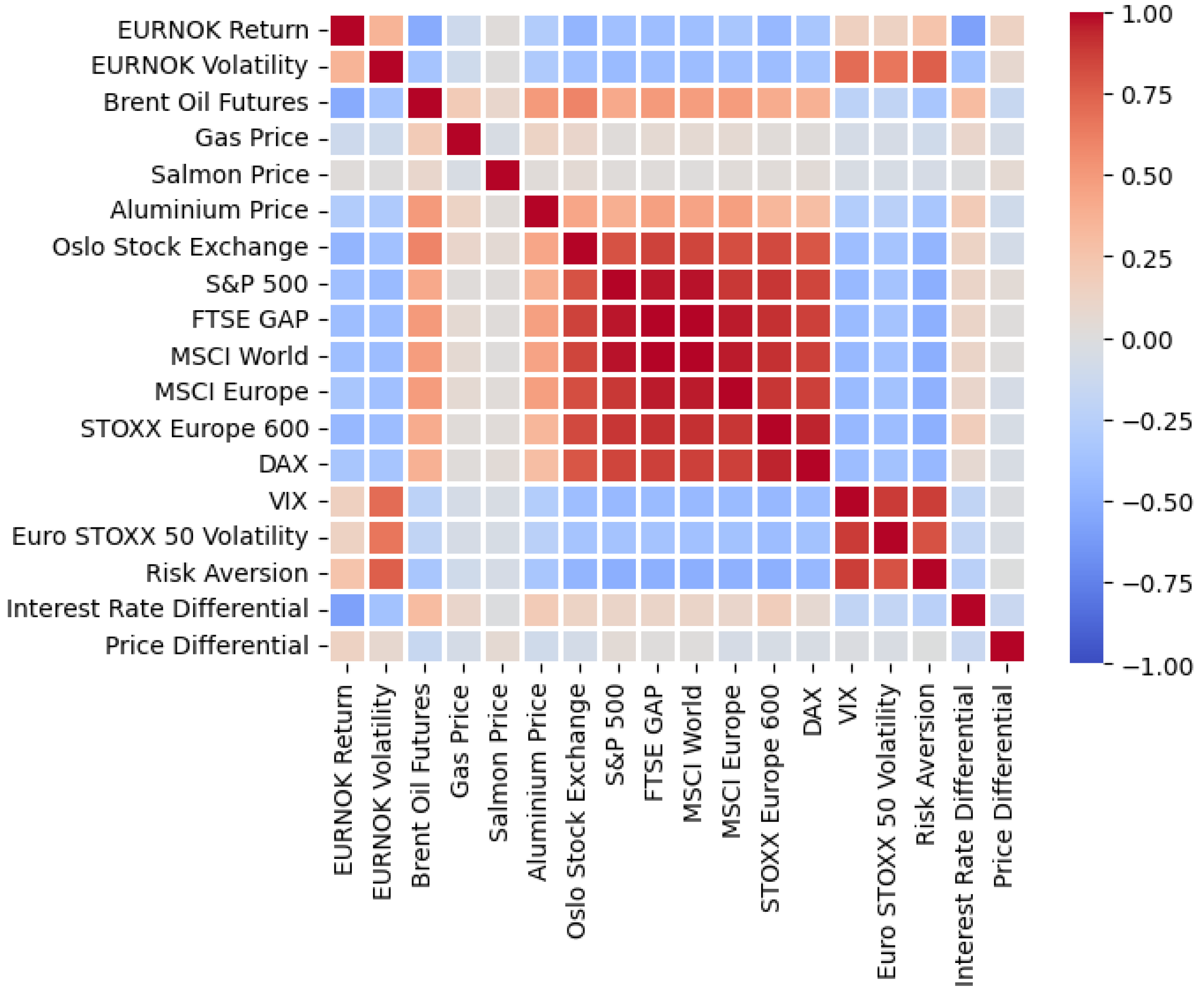
3.3. Explanatory Variables

3.3.1. Commodities

We included the oil price, represented by the 1st ICE Brent Crude Futures, in our analysis. The export value of Natural Gas has increased over time, equaling 34.5% of Norway’s total export in 2021. Hence, we included the Henry Hub spot price. Furthermore, we included salmon and aluminum spot prices, which constitute significant portions of Norwegian exports.

3.3.2. Financial Assets

In line with the literature, we included the S&P 500 index as an explanatory variable. However, we included other equity indices as well: the FTSE Global All Cap (FTSE GAP), MSCI World, MSCI Europe, Stoxx Europe 600, Dax, and Oslo Stock Exchange. The argument for investigating more indices is that S&P 500 only includes American companies, and we wish to investigate whether indices representing other parts of the world yield different results.

3.3.3. Financial Uncertainty

As volatility indices, we included VIX and Euro Stoxx 50 Volatility, which are the indices for the S&P 500 and Euro Stoxx 50, respectively. In addition to volatility indices, we included a variable that measures market risk aversion. The latent relationship between market sentiment and asset prices is most likely complex and non-linear. To represent risk aversion, we employed the index proposed by Bekaert et al. (2022). The index is constructed using six financial variables, namely, the term spread, credit spread, detrended dividend yield, realized and risk-neutral equity return variances, and realized corporate bond return variance. This risk aversion index is based on U.S. market data, and given the size and importance of U.S. capital markets, we interpret the index as a proxy for global risk aversion. This index has not previously been investigated in the context of Norwegian krone returns.

3.3.4. Macroeconomic Fundamentals

Due to the fundamental theories on PPP and UIP and the consensus on their relevance for exchange rate modeling, we included both price and interest differentials as explanatory variables. The price differential is the difference between the price level in Norway and the euro area, using the harmonized consumer price index (HCPI). For interest rates, we used the 12-month NIBOR and EURIBOR, which are the Norwegian and Euro Interbank Offered Rates, respectively.

4. Methodology

The empirical approach in Section 4.1 broadly follows Hollstein et al. (2021).2 Univariate models are useful for the purpose of this study, as they allow us to analyze time variation in covariances between a single explanatory variable and the dependent variable. Furthermore, we assessed whether the time variation in covariances arises solely from the time variation in the volatilities or whether correlation has its own dynamic pattern. For this purpose, we employed the Dynamic Conditional Correlation model proposed by Engle (2002), briefly outlined in Section 4.2.

4.1. Univariate Regression

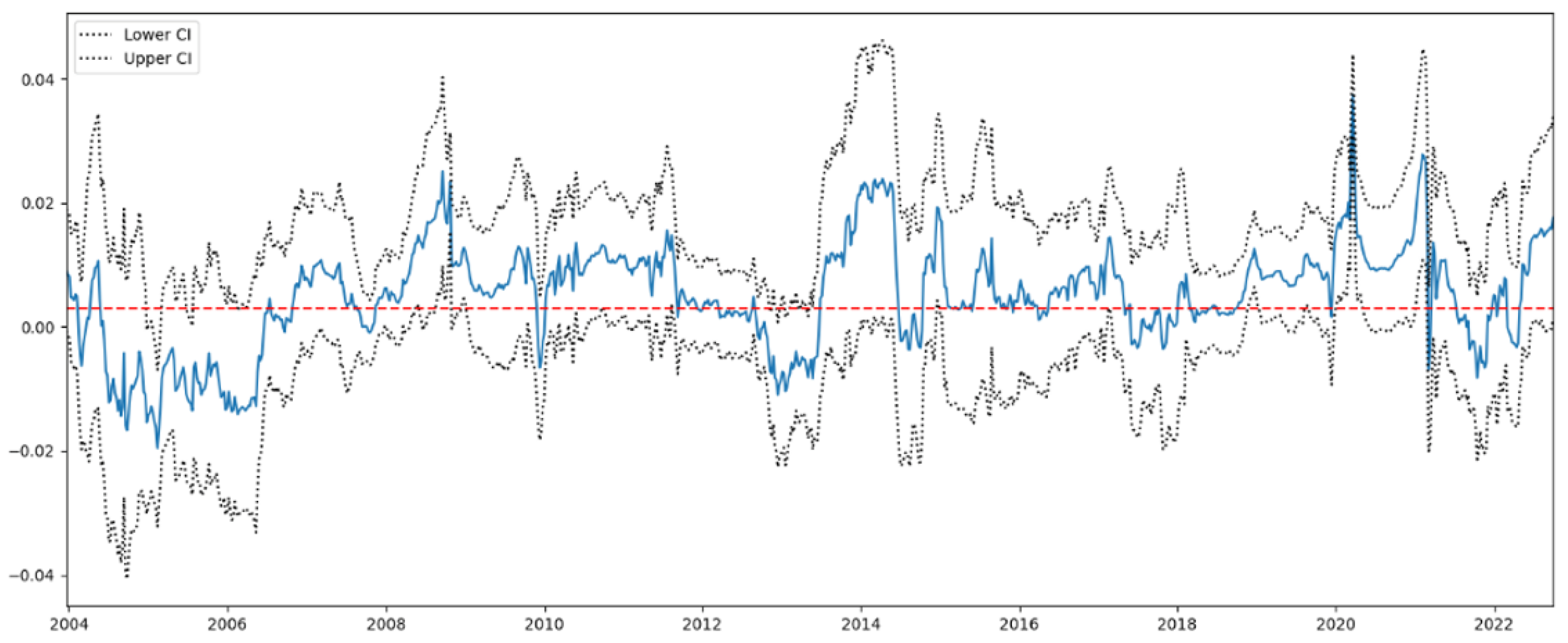
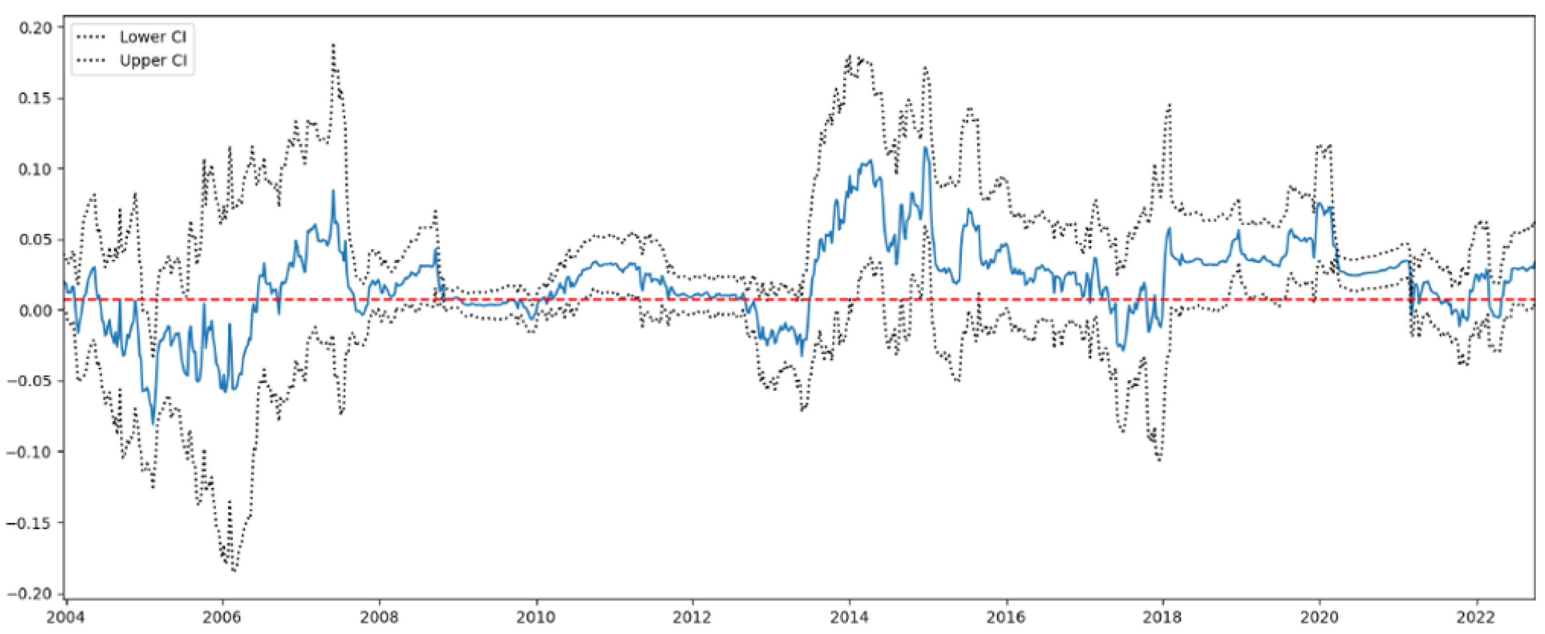
4.1.1. Time-Varying Relationship

In our analysis of the potential time-varying relationship between the explanatory and explained variables, we used univariate rolling OLS regression. We estimated the model parameters from k initial observations, where k is the number of periods in a rolling window. For the following period, we rolled the estimation period by one and re-estimated the model. This gives us T k distinct regressions for each variable, where T is the total number of observations. We estimated models for both weekly and monthly data. For the weekly models, we used a rolling regression window of 50 weeks. For the monthly models, the windows were set to 30 months. In general, capturing time dependencies in regression coefficients requires frequent re-estimation and relatively short estimation windows while avoiding high variance in coefficients. Rolling estimation windows of 50 and 30 weeks yield an appropriate balance between these two considerations in our research design.
To assess the relationship between the explanatory variables and EURNOK return, we fit the following regression model:
R t = α + β X t + ϵ t
where R t is the periodic (average) return from period t 1 to t, α and β are the intercept and slope parameters, respectively, X t is the explanatory variable at time t, and ϵ t represents the regression error term. When evaluating the regressions, we had two main areas of interest. Firstly, we analyzed the goodness of fit. Secondly, we assessed the time-varying relationship between the explained variable and the explanatory variable.
We used R 2 as a measure of goodness of fit and computed R 2 for all T k periods. By plotting R 2 values over time, we can visualize how the explanatory power of the regression model changes during the time period. For instance, if the plotted R 2 values show a generally increasing trend over time, this suggests that the model is becoming more effective at explaining the relationship between the explained and explanatory variables. On the other hand, if the plotted R 2 values show a generally decreasing trend, this suggests that the model is becoming less effective over time.
To evaluate the relationship between the explained and explanatory variables, we examined the β parameter. We obtained the estimated β parameters and calculated 95% confidence intervals for all T k time periods. We plotted the estimated β values over time. If the plotted values form a relatively flat line, this suggests that the relationship is relatively constant. However, if the plotted values show significant changes over time, this suggests that the relationship is time-varying.

4.1.2. Predictability

We started our exploration of return predictability with an in-sample ( I S ) analysis. For the I S predictability, we estimated the following regression model with 1-month/1-week-ahead return on a constant and the predictor variable:
R t + 1 = α + β X t + u t + 1
where R t + 1 is the monthly/weekly (average) return from month/week t to t + 1 , and α and β are the intercept and slope parameters. X t is the predictor variable at time t, and u t + 1 is a disturbance term. We followed Rapach and Wohar (2006) and assessed the predictive ability of X t by examining β ^ . Under the null hypothesis of no predictability, β ^ is not significantly different from zero, whereas under the alternative hypothesis, β ^ is different from zero. We assessed statistical significance using a t-test from a bootstrapped distribution.3 Note that for the initial I S analysis of return, we did not use a rolling window.
For the out-of-sample ( O O S ) forecast, we estimated Equation (2) using a rolling window. The initial parameters were estimated from the k initial observations. The first forecast was given by the most recent observations of the predictor variable and the generated parameter values. For the next prediction, we rolled the estimation period by one and generated updated parameters. We then estimated models for weekly and monthly data. For the weekly models, we used a rolling regression window of 50 weeks. For the monthly models, the window was 30 months.
We evaluated whether the variables have predictive properties by comparing the model to a naive benchmark, under which the best estimator for future expected return is the recursive mean. We followed Campbell and Thompson (2008) and used the out-of-sample fit of the measure R O O S 2 , given by:
R O O S 2 = 1 M S E u M S E r
where M S E u and M S E r are the mean squared errors of the unrestricted and restricted models, respectively. The unrestricted model is given by Equation (2). Similarly, the restricted model is the historical mean, corresponding to setting β in Equation (2) equal to zero. If R O O S 2 from Equation (3) is positive, the unrestricted model predicts future returns more accurately than the restricted model.
To evaluate O O S predictability, we used the MSE-F statistic of McCracken (2007), in combination with the bootstrap approach of Rapach and Wohar (2006):
M S E F = ( N k + 1 ) × ( M S E r M S E u M S E u )
where N is the number of O O S forecasts, and k is the forecast window (k = 1 in our case).
Furthermore, we included two forecast combinations; “Combination All” and “Combination Selected”. The former is a simple mean forecast, computed as the average across all univariate O O S models. The latter selects only the predictors that yield a positive R O O S 2 value and computes the mean of their predictions.

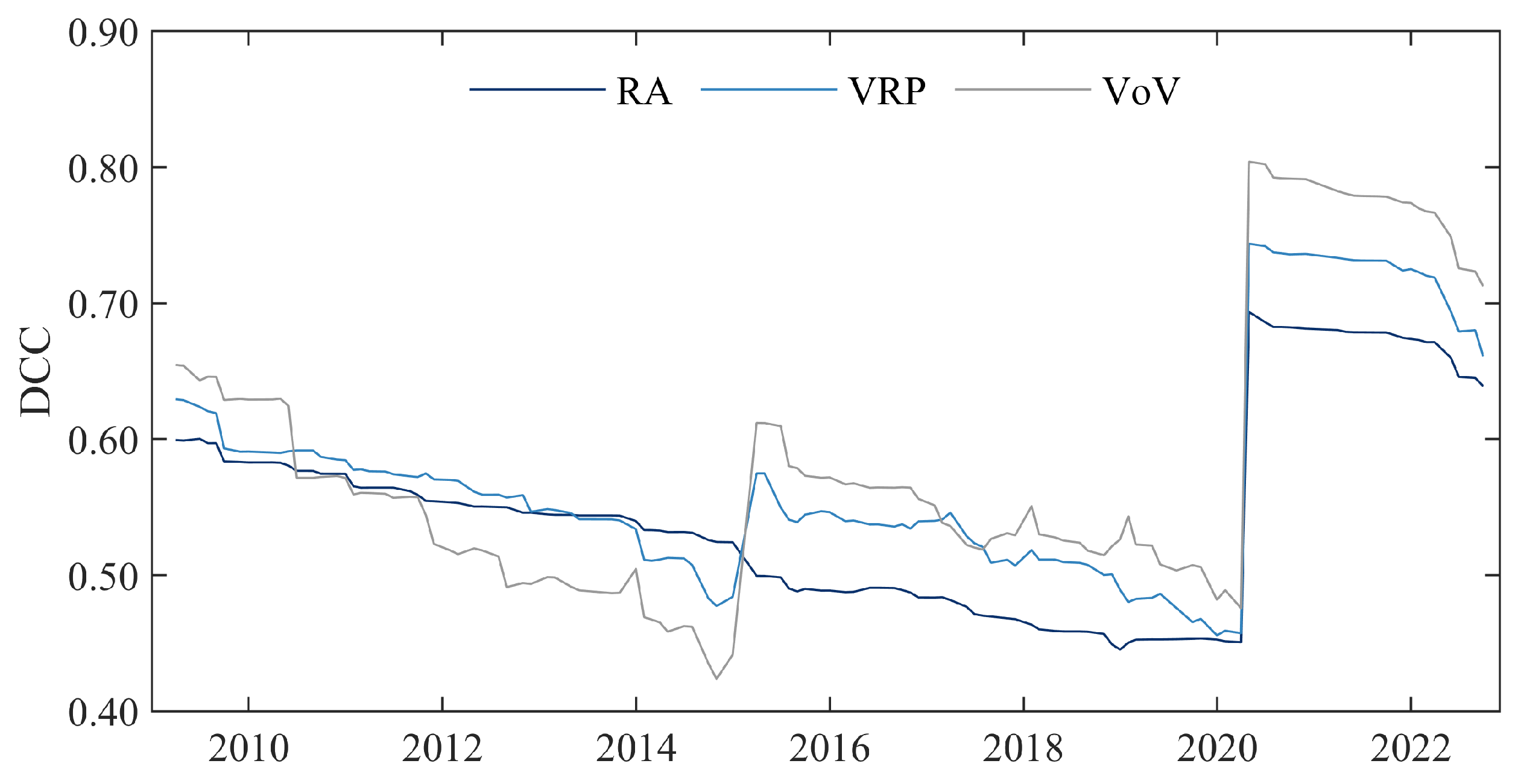
4.2. Dynamic Conditional Correlation

The Dynamic Conditional Correlation (DCC) model (Engle 2002) allows for the estimation of the conditional correlation between each pair of variables in a multivariate series, taking into account the dynamic nature of the correlation and the presence of conditional heteroskedasticity. In the DCC model, the conditional correlation matrix follows a time-varying autoregressive process.
Given standardized residuals obtained from univariate GARCH models, the conditional correlation matrix, denoted by Q t , is estimated using the DCC equation:
Q t = D t · R t · D t ,
where D t is a diagonal matrix containing the conditional standard deviations, and R t is the conditional correlation matrix at time t. The conditional correlation matrix is estimated as:
R t = ( 1 λ ) · R ¯ + λ · Q t 1 ,
where R ¯ is the long-run average correlation matrix, and λ is a constant between 0 and 1, representing the speed of adjustment of the correlation matrix.

5. Results and Discussion

5.1. Time-Varying Relationship

Table 3 reports R 2 for all variables under consideration, computed from the univariate regression model in Equation (1). We report the mean (taken as the equal-weighted average of R 2 over all rolling window estimates), minimum, and maximum.
As evident from Table 3, the linear dependency—as measured by R 2 —varies over time. All variables have an R 2 close to zero at some point during the sample period. This is as expected since using only one variable to model exchange rates has generally not yielded accurate results. However, by investigating the mean value, we obtain a consistent picture of which variables are most strongly associated with EURNOK returns. Comparing weekly and monthly values, we notice that the monthly values tend to be a bit higher for most of the variables, suggesting that more frequent samples do not give better results for this model.
Figure 2 shows how the coefficient of Brent Oil Futures has evolved. The average β for the whole period, computed without a rolling window, is marked by the red dotted line, just below −0.1. This negative correlation is consistent with other studies, where an increase in the oil price results in an appreciation of the krone against the euro. Using the average value, an increase in the oil price of 1% results in a decrease in EURNOK of 0.1%. The rolling window regression mainly evolves around the average, with a few spikes, and the confidence interval captures the average at almost all time periods. However, we see a weak tendency for more negative values in recent years. Most notably, we note a significant change in mid-2015, where β changes from being positive to its most negative value during the whole sample period.
The other commodity prices do not appear to have any significant contemporaneous relationship with EURNOK returns.
Investigating Figure 3, we see that the average coefficient for the Oslo Stock Exchange is negative 0.2, suggesting that an increase in the index of 1% on average is associated with a 0.2% decrease in EURNOK returns. The results for the other equity indices are similar.4 In addition, given the typical interpretation of S&P 500 as a proxy for global equities, it is interesting to note that S&P 500 has a lower average value than the majority of the other indices.
The perceived level of risk is known to impact investor portfolio allocations and, consequently, returns. Although the level of risk is a latent variable, we represent this by the VIX index and by the risk aversion index proposed by Bekaert et al. (2022).
Figure 4 shows that the average β -coefficient of VIX is close to zero. The development of β for the risk aversion index illustrated in Figure 5 displays a distinctly different pattern. From 2008 to 2014, a period characterized by modest volatility across asset classes and extraordinary monetary policy measures in the forms of unprecedentedly low short-term interest rates and quantitative easing, EURNOK returns do not appear to have been related to risk aversion. Since 2014, however, the β -coefficient has been positive. Furthermore, the magnitude of the coefficient increases sharply during periods of financial distress, such as the global financial crisis, Brexit, and the COVID-19 outbreak. It is also interesting to note that the sign of the β -coefficient changes from negative to positive for both VIX and risk aversion during the global financial crisis.
Figure 2, Figure 3, and Figure 5 strongly suggest that a structural shift occurred around 2015. To investigate this further, we performed a subsample analysis. Table 4 shows that the average β is considerably more negative after 2015, especially for the Oslo Stock Exchange. The average degree of explainability increases for both Brent Futures and the Oslo Stock Exchange. To test whether the change is significant, we performed a Chow test, and as the p-value shows, the difference before and after 2015 is statistically significant at a 1% level for both variables. The same is true for all other financial assets included in our analysis, and we have included FTSE GAP for illustrative purposes. Another variable where the Chow test shows that the change is statistically significant before and after 2015 is the risk aversion index. As the table shows, both β and R 2 are relatively close to zero compared to the other variables. However, we see that the average values of both β and R 2 increase, suggesting that the relevance of risk aversion for EURNOK returns has become greater.
Figure 6 illustrates how the coefficient of the interest rate differential evolves over the sample period. The negative coefficient is consistent with the UIP, which states that a larger difference will result in an appreciation of the krone. We notice more deviation from its average after 2014.
Table 3 shows that the price differential has low R 2 values.

5.2. Predictability

Table 5 illustrates how our model performs compared to a naive benchmark in terms of predictability. A few common observations emerge: For most of the variables, the naive benchmark outperforms our model. This is not surprising, given the consensus in the literature that multivariate models, taking into account variable co-dependencies, are most appropriate. Furthermore, most variables display in-sample predictability, expressed by R I S 2 . However, as indicated by the negative R O O S 2 , this predictability tends to disappear in out-of-sample forecasts.
For the monthly O O S analysis, all variables have negative R O O S 2 values, which is why “Combination Selected” is empty. However, the analysis performed with a weekly frequency shows that two variables, namely, Oslo Stock Exchange and Stoxx Europe 600, outperform the benchmark model and are statistically significant at the 1% level. Since they inhibit a larger degree of explainability on EURNOK returns than many other variables, it is not impossible that they also have some predictive properties. Overall, most variables show slightly better results when using data with a weekly frequency, suggesting that more frequent data points could prove beneficial when predicting EURNOK returns.

5.3. Dynamic Conditional Correlations (DCCs)

To isolate conditional correlations from conditional volatilities, we utilized the DCC framework, briefly outlined in Section 5.3. For the univariate GARCH models, we assumed GARCH(1,1) processes with Student-t-distributed residuals. Furthermore, we assumed a multivariate t distribution for the joint conditional distributions and a lag order equal to one for the autoregressive conditional correlation matrix.
Figure 7 shows the Dynamic Conditional Correlations of the most important explanatory variables identified in Section 4.1, based on monthly observations over the full sample period.
In Section 4.1, we capture time variation by re-estimating the regression models. In this section, we take an alternative approach, as we control for conditional volatility over the full sample, thus obtaining conditional linear correlations. Figure 7 is consistent with the findings in Section 4.1. As is well established in the existing literature, EURNOK returns exhibit negative correlations with changes in the oil price and asset prices. This paper is the first to quantify a positive association between market risk aversion, as proxied by the index proposed by Bekaert et al. (2022), and EURNOK returns. Most notably, Figure 7 shows that these correlations tend to increase during turbulent periods, most notably during the global financial crisis and the COVID-19 outbreak, which is consistent with well-established stylized facts from other markets.

5.4. Risk Aversion Robustness Analysis

As shown in Section 4.1 and Section 4.2, EURNOK returns are negatively correlated with risk aversion, as proxied by the index in Bekaert et al. (2022). This index is based on U.S. data, and although we consider it a representative measure of global risk aversion, it might be less relevant for Norwegian currency. Furthermore, risk aversion is a latent variable, and any proxy suffers from this inherent problem. Hence, as a robustness test, we considered alternative measures of risk aversion and compared them using the DCC framework.
Bollerslev et al. (2009) and Bekaert and Hoerova (2014), among others, interpret the variance risk premium (VRP) as the price of market risk, hence reflecting risk aversion. The market price of variance risk is simply defined as the difference between the risk-neutral and physical expectations of variance:
V R P t , T = E t Q ( V t , T 2 ) E t P ( V t , T 2 ) ,
where V t , T 2 refers to return variation. E t Q ( V t , T 2 ) is the ex ante forecast of the variance under the risk-neutral probability, which is measured by the implied volatility of 1-month EURNOK at-the-money options. E t P ( V t , T 2 ) is the ex ante forecast of the variance under the physical measure, proxied by the ex post realized variance R V t .5 The expected variance risk premium is thus given by:
V R P t I V t 2 R V t ,
where I V t 2 and R V t are scaled to a monthly frequency.
Baltussen et al. (2018) introduced the volatility-of-volatility (VoV) as measure of risk aversion, subsequently employed in empirical analyses by Hollstein et al. (2019) and Jeon et al. (2020), among others. The volatility-of-volatility is computed as
V o V t = 1 21 Σ i = t 21 σ i σ ¯ t I V σ t I V ¯ ,
where σ t I V ¯ = 1 21 Σ i = t 21 σ i , and σ i is the implied volatility of 1-month EURNOK at-the-money options.
In our analysis, VRP and VoV can be interpreted as idiosyncratic measures of EURNOK risk aversion, whereas RA proxies global risk aversion. From Figure 8, it is it clear that the three measures of risk aversion are highly correlated. It is noteworthy, though, that VRP and VoV spike following the 2014 rapid decline in oil prices, which proved harmful to the oil-related sectors of the Norwegian economy. All three measures display high and increasing correlations with EURNOK returns following COVID-19, confirming our findings in Section 4.1 that the depreciation of EURNOK is associated with increased risk aversion, supporting the view that the Norwegian krone is no longer a safe-haven currency.6

5.5. Discussion

The empirical results outlined in Section 5 suggest that EURNOK returns are associated with changes in commodity prices, financial assets, financial uncertainty, and macroeconomic fundamentals. A negative relationship between EURNOK returns and Brent, where an increase in the oil price coincides with an appreciation of the krone, is consistent with the existing literature. Other commodity prices do not appear to have any significant contemporaneous relationship with EURNOK returns. A plausible explanation for this could be that oil makes up a much larger part of the total export value than gas, aluminum, and salmon.
On average, we find a negative relationship between equity indices and EURNOK returns. This is somewhat contrary to Naug (2003) and Benedictow and Hammersland (2022), who report that an increase in the S&P 500 relates to a depreciation of the krone. In Figure 3, we see that the sign of the OSE β coefficient changes from positive to negative after the 2008 financial crisis. Furthermore, there has been a tendency for a stronger negative correlation in more recent years. Thus, our rolling window regression captures a change in the dynamics in EURNOK returns. For OSE and FTSE GAP, structural shifts occur around 2014. The β coefficients shift markedly downward and remain below average. This coincides with the rapid 2015 decline in global oil prices, which triggered a restructuring of the Norwegian offshore supply sector. Correspondingly, the transition to green energy has been intensified over time. One possible effect of this is that markets assign less value to Norwegian fossil energy reserves, rendering the oil price less important for EURNOK. In total, we interpret our results as evidence that the sensitivity of EURNOK to equity prices has increased over time.
One novelty in this paper is the assessment of the impact of financial uncertainty. β , used for the risk aversion index, as illustrated in Figure 5, changes significantly around 2014, corresponding in time to the Oslo Stock Exchange β shift. The positive correlation after 2014 suggests that when the market risk aversion increases, the krone will depreciate. The development of β differs from that of VIX, which is illustrated in Figure 4. This might suggest that it is not necessarily increased market uncertainty that is the main driver of EURNOK returns, but rather the risk aversion of investors.
From the perspective of considering whether the Norwegian krone is considered a safe-haven currency, it is interesting to analyze the development of the regression coefficient of risk aversion on EURNOK returns in Figure 5. Prior to the global financial crisis, the sign of the coefficient was negative, implying that higher risk aversion attracted NOK buyers. However, the signed switched during the financial crisis and has remained positive since. Furthermore, the magnitude of the positive coefficient increases sharply during periods of financial distress, such as the global financial crisis, the 2014 oil price decline, Brexit, and the COVID-19 outbreak. We interpret this as evidence of the krone changing characteristics from a safe-haven currency to a more peripheral and risk-exposed currency. This conclusion is robust to other measures of risk aversion, as confirmed by the analysis of Dynamic Conditional Correlations displayed in Figure 8.
Since oil price and equity indices on average have the highest R 2 , we investigated the development of these values more closely. Figure 9 and Figure 10 illustrate how the R 2 values evolve over time. We notice that both have spikes around 2015 and 2020, suggesting a higher correlation with EURNOK returns during these periods. For the Oslo Stock Exchange, we also see a spike during 2008. It is minor compared to the others, but based on the R 2 values prior to 2008, it is significant. The spikes occur in periods with high market uncertainty, with the financial crisis in 2008, the drop in the oil price in late 2014, and the COVID-19 pandemic in 2020. We interpret the fact that changes in both the oil price and financial assets have higher correlations with EURNOK returns during these periods as indications of regime-switching behavior of EURNOK returns.
Even though we observe that certain variables are associated with EURNOK returns, this does not generally carry over to out-of-sample predictability. This is somewhat unsurprising. Since Rogoff (1996), it has been well known that the random walk is hard to beat when forecasting FX returns, even when complex multivariate models are applied.

6. Conclusions

This study utilized a broad set of variables to investigate time-varying relationships with EURNOK returns and the related predictability. We find that changes in the oil price, financial assets, and risk aversion contain the highest explanatory power for EURNOK returns. We observe that the relative importance of financial assets has increased over time, supporting a view that the Norwegian economy is transforming from being commodity-based into being more exposed to global asset prices. Furthermore, we observe that risk aversion is important for EURNOK returns—a conclusion that is robust with respect to the choice of risk aversion proxy. More specifically, our empirical analysis indicates that the krone is no longer a safe-haven currency. In line with the body of literature, this study confirms that FX returns are generally unpredictable.
The results of this study can be extended in several directions. Further analysis of the impact of risk aversion might enhance our understanding of the dynamics of small, open-commodity-based currencies in general, such as CAD, NZD, and AUD. Specifically for EURNOK, the empirical analysis in this paper shows that risk aversion is particularly relevant during turbulent periods. This insight can be exploited by practitioners for the purpose of modeling the EURNOK risk–reward. Furthermore, the relationship between EURNOK and other financial variables is most likely complex and non-linear. As such, state-space models and Bayesian vector autoregressive models, possibly based on principal component analysis, might prove helpful. In addition, forecast error decomposition might shed additional light on the dynamics of EURNOK returns. We leave this for further research.

Author Contributions

Conceptualization, M.R. and S.W.; methodology, M.R., A.T. and K.A.T.; software, A.T. and K.A.T.; formal analysis, A.T. and K.A.T.; investigation, A.T. and K.A.T.; data curation, M.R., A.T. and K.A.T.; writing—original draft, M.R. and K.A.T.; writing—review and editing, S.W.; supervision, M.R. and S.W.; project administration, M.R. and S.W. All authors have read and agreed to the published version of the manuscript.

Funding

This research received no external funding.

Data Availability Statement

We do not have permission to share the data employed in this study.

Conflicts of Interest

The authors declare no conflict of interest.

Notes

1
I44 is a nominal effective krone exchange rate calculated on the basis of NOK exchange rates against the currencies of Norway’s 25 main trading partners (Norges Bank 2023).
2
Using more than 140 years of data, they analyzed the predictive power of a broad set of business cycle variables for risk and return in commodity spot markets. They found statistically significant predictors for both commodity returns and commodity volatilities using univariate rolling OLS regression models.
3
See Section 2.3 of Rapach and Wohar (2006).
4
Available from the corresponding author upon request.
5
As is common in the literature, we estimated R V t from high-frequency data sampled at a 5-minute frequency (Andersen et al. 2001; Liu et al. 2015). To filter the tick-level data, we started by applying the cleaning procedure suggested by Barndorff-Nielsen et al. (2009), which is summarized as follows: First, we deleted entries with (i) zero quotes, (ii) a negative bid–ask spread, (iii) a bid–ask spread greater than 50 times the median spread on that day, and (iv) a mid-quote that deviates by more than 10 mean absolute deviations from the centered mean (excluding the observation under consideration) of 25 observations before and 25 observations after. Second, we computed mid-quotes as the average of the bid and ask quotes and resampled the data using a 5 min frequency. The data are publicly available at DukasCopy (accessed 10 January 2023).
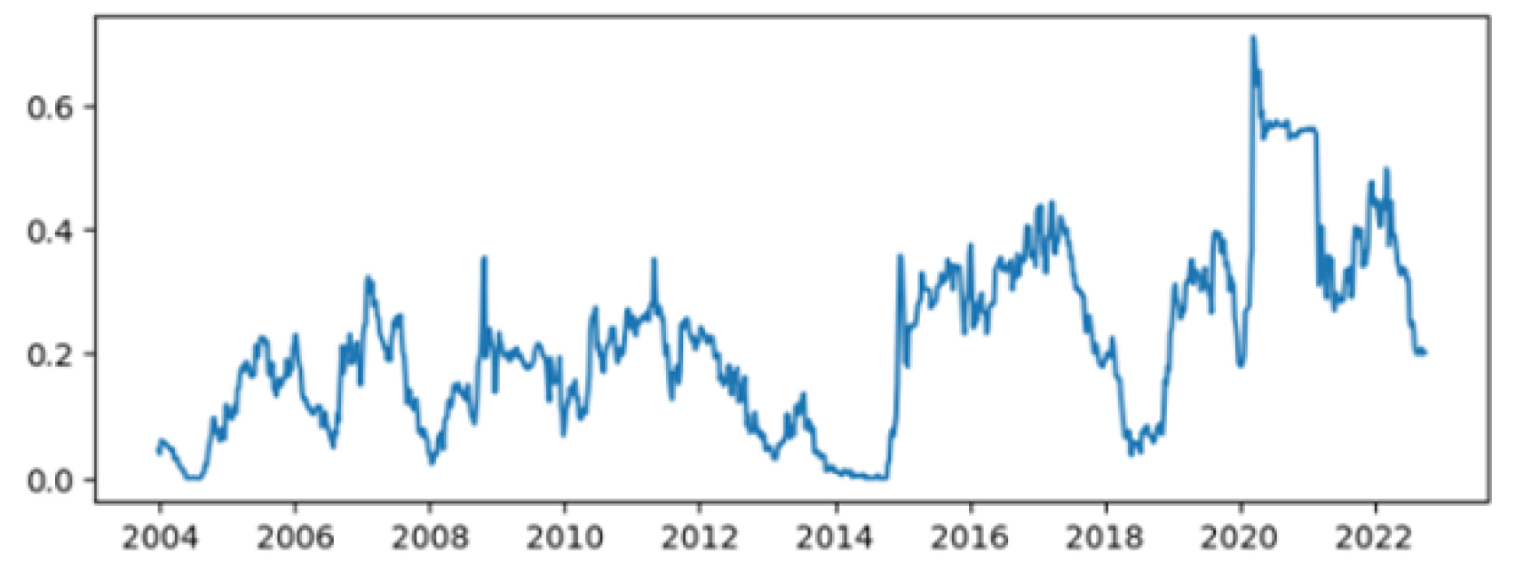
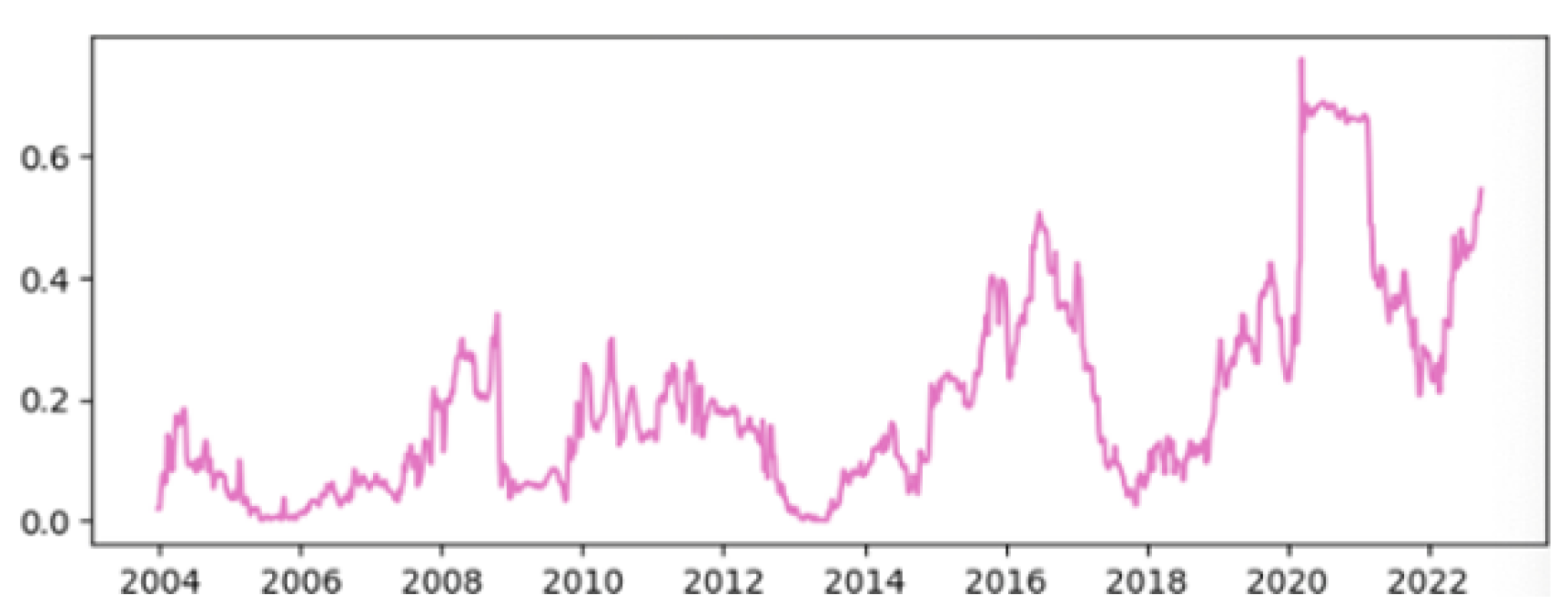
6
Note that, due to the availability of data, the sample underlying Figure 8 covers June 2009 to September 2022, i.e., slightly shorter than the full sample period from January 2003 to September 2022 applied elsewhere in the paper.

References

  1. Akram, Q. Farooq. 2006. PPP in the medium run: The case of norway. Journal of Macroeconomics 28: 700–19. [Google Scholar] [CrossRef]
  2. Akram, Q. Farooq. 2020. Oil price drivers, geopolitical uncertainty and oil exporters’ currencies. Energy Economics 89: 104801. [Google Scholar] [CrossRef]
  3. Aloosh, Arash, and Geert Bekaert. 2022. Currency factors. Management Science 68: 4042–64. [Google Scholar] [CrossRef]
  4. Andersen, Torben G., Tim Bollerslev, Francis X. Diebold, and Paul Labys. 2001. The distribution of realized exchange rate volatility. Journal of the American Statistical Association 96: 42–55. [Google Scholar] [CrossRef]
  5. Baltussen, Guido, Sjoerd Van Bekkum, and Bart Van Der Grient. 2018. Unknown unknowns: Uncertainty about risk and stock returns. Journal of Financial and Quantitative Analysis 53: 1615–51. [Google Scholar] [CrossRef] [Green Version]
  6. Barndorff-Nielsen, Ole E., P. Reinhard Hansen, Asger Lunde, and Neil Shephard. 2009. Realized kernels in practice: Trades and quotes. The Econometrics Journal 12: C1–C32. [Google Scholar] [CrossRef]
  7. Bekaert, Geert, and Marie Hoerova. 2014. The vix, the variance premium and stock market volatility. Journal of Econometrics 183: 181–92. [Google Scholar] [CrossRef] [Green Version]
  8. Bekaert, Geert, Eric C. Engstrom, and Nancy R. Xu. 2022. The time variation in risk appetite and uncertainty. Management Science 68: 3975–4004. [Google Scholar] [CrossRef]
  9. Benedictow, Andreas, and Roger Hammersland. 2022. Why Has the Norwegian Krone Exchange Rate Been Persistently Weak? A Fully Simultaneous VAR Approach. Technical Report, Statistics Norway, Discussion Papers. Available online: https://www.ssb.no/en/nasjonalregnskap-og-konjunkturer/konjunkturer/artikler/why-has-the-norwegian-krone-exchange-rate-been-persistently-weak-a-fully-simultaneous-var-approach/_/attachment/inline/f1c08d6c-7a4b-4e14-93ec-f410095f9411:c9e0e487e483c7bd265aae1205aaab247a410634/DP981_web.pdf (accessed on 1 February 2023).
  10. Bernhardsen, Tom, and Oistein Roisland. 2000. Factors that influence the krone exchange rate. Economic Bulletin 71: 143. [Google Scholar]
  11. Bollerslev, Tim, George Tauchen, and Hao Zhou. 2009. Expected stock returns and variance risk premia. The Review of Financial Studies 22: 4463–92. [Google Scholar] [CrossRef]
  12. Campbell, John Y., and Samuel B. Thompson. 2008. Predicting excess stock returns out of sample: Can anything beat the historical average? Review of Financial Studies 21: 1509–31. [Google Scholar] [CrossRef] [Green Version]
  13. Engle, Robert. 2002. Dynamic conditional correlation: A simple class of multivariate generalized autoregressive conditional heteroskedasticity models. Journal of Business & Economic Statistics 20: 339–50. [Google Scholar]
  14. Flatner, Alexander, Preben Holthe Tornes, and Magne Østnor. 2010. En oversikt over Norges Banks Analyser av Kronekursen. Norges Bank Staff Memo, 7/2010. Available online: https://norges-bank.brage.unit.no/norges-bank-xmlui/bitstream/handle/11250/2507760/staff_memo_0710.pdf?sequence=1&isAllowed=y (accessed on 1 February 2023).
  15. Furuseth, Thomas. 2022. Hvorfor er den norske krona så svak? DnB Analyst Report. Available online: https://www.dnb.no/dnbnyheter/no/bors-og-marked/hvorfor-er-den-norske-krona-saa-svak-mkts (accessed on 1 February 2023).
  16. Hollstein, Fabian, Duc Binh Benno Nguyen, and Marcel Prokopczuk. 2019. Asset prices and “the devil (s) you know”. Journal of Banking & Finance 105: 20–35. [Google Scholar]
  17. Hollstein, Fabian, Marcel Prokopczuk, Björn Tharann, and Chardin Wese Simen. 2021. Predictability in commodity markets: Evidence from more than a century. Journal of Commodity Markets 24: 100–71. [Google Scholar] [CrossRef]
  18. Jeon, Byounghyun, Sung Won Seo, and Jun Sik Kim. 2020. Uncertainty and the volatility forecasting power of option-implied volatility. Journal of Futures Markets 40: 1109–26. [Google Scholar] [CrossRef]
  19. Jiang, Zhengyang, and Robert J. Richmond. 2023. Origins of international factor structures. Journal of Financial Economics 147: 1–26. [Google Scholar] [CrossRef]
  20. Klovland, Jan Tore, Lars Myrstuen, and Didrik Sylte. 2021. Den svake norske kronen—Fakta eller fiksjon? Samfunnsøkonomen 2: 9–20. [Google Scholar]
  21. Liu, Lily Y., Andrew J. Patton, and Kevin Sheppard. 2015. Does anything beat 5-minute rv? A comparison of realized measures across multiple asset classes. Journal of Econometrics 187: 293–311. [Google Scholar] [CrossRef] [Green Version]
  22. Lustig, Hanno, and Robert J. Richmond. 2020. Gravity in the exchange rate factor structure. The Review of Financial Studies 33: 3492–540. [Google Scholar] [CrossRef]
  23. Lustig, Hanno, Nikolai Roussanov, and Adrien Verdelhan. 2011. Common risk factors in currency markets. The Review of Financial Studies 24: 3731–77. [Google Scholar] [CrossRef]
  24. Lustig, Hanno, Nikolai Roussanov, and Adrien Verdelhan. 2014. Countercyclical currency risk premia. Journal of Financial Economics 111: 527–53. [Google Scholar] [CrossRef] [Green Version]
  25. Martinsen, Kjetil. 2017. Norges Bank’s BEER Models for the Norwegian Effective Exchange Rate. Norges Bank Staff Memo, No. 7/2017. Available online: https://www.econstor.eu/handle/10419/210341 (accessed on 1 February 2023).
  26. Maurer, Thomas A., Thuy-Duong Tô, and Ngoc-Khanh Tran. 2019. Pricing risks across currency denominations. Management Science 65: 5308–36. [Google Scholar] [CrossRef]
  27. McCracken, Michael W. 2007. Asymptotics for out of sample tests of granger causality. Journal of Econometrics 140: 719–52. [Google Scholar] [CrossRef]
  28. Meese, Richard A., and Kenneth Rogoff. 1983. Empirical exchange rate models of the seventies. Journal of International Economics 14: 3–24. [Google Scholar] [CrossRef]
  29. Naug, Bjørn E. 2003. Factors behind movements in the krone exchange rate—An empirical analysis. Norges Banks Skriftserie 32: 115–35. [Google Scholar]
  30. Norges Bank. 2023. TWI, Trade Weighted Exchange Rate. Available online: https://www.norges-bank.no/en/topics/Statistics/twi/ (accessed on 1 February 2023).
  31. Rapach, David E., and Mark E. Wohar. 2006. In-sample vs. out-of-sample tests of stock return predictability in the context of data mining. Journal of Empirical Finance 13: 231–47. [Google Scholar] [CrossRef]
  32. Rogoff, Kenneth. 1996. The purchashing power parity puzzle. Journal of Economic Literature 34: 647–68. [Google Scholar]
  33. Sarno, Lucio. 2005. Towards a solution to the puzzles in exchange rate economics: Where do we stand? The Canadian Journal of Economics 38: 673–708. [Google Scholar] [CrossRef]
  34. Taylor, Mark P. 2003. Purchasing power parity. Review of International Economics 11: 436–52. [Google Scholar] [CrossRef]
  35. Verdelhan, Adrien. 2018. The share of systematic variation in bilateral exchange rates. The Journal of Finance 73: 375–418. [Google Scholar] [CrossRef]
Figure 1. Pairwise correlation of all variables for monthly values. The correlation matrix for weekly values is practically identical.
Jrfm 16 00308 g001
Figure 2. Slope coefficient of Brent Oil Futures on EURNOK returns.
Jrfm 16 00308 g002
Figure 3. Slope coefficient of Oslo Stock Exchange on EURNOK returns.
Jrfm 16 00308 g003
Figure 4. Slope coefficient of VIX on EURNOK returns.
Jrfm 16 00308 g004
Figure 5. Slope coefficient of risk aversion index on EURNOK returns.
Jrfm 16 00308 g005
Figure 6. Slope coefficient of interest rate differential on EURNOK returns.
Jrfm 16 00308 g006
Figure 7. Dynamic Conditional Correlations of EURNOK and Brent (top panel); OSEAX, FTSE GAP, and MSCI (middle panel); and the risk aversion index of Bekaert et al. (2022) (lower panel). Monthly data over the full sample.
Jrfm 16 00308 g007
Figure 8. Dynamic Conditional Correlations of alternative proxies for risk aversion. RA: The risk aversion index of Bekaert et al. (2022). VRP: The variance risk premium from 1-month EURNOK options, as per Equation (6). VoV: The uncertainty of 1-month EURNOK implied volatilities, as per Equation (7). Monthly data from June 2009 to September 2022.
Jrfm 16 00308 g008
Figure 9. R 2 Brent Oil Futures.
Jrfm 16 00308 g009
Figure 10. R 2 Oslo Stock Exchange.
Jrfm 16 00308 g010
Table 1. Literature overview.
ReferencePeriodMethodMain Explanatory Variables
Naug (2003)2000–2003 MonthlyECMInterest rate differential. Oil price. S&P 500. A global hazard indicator.
Bernhardsen and Roisland (2000)1993–2000 MonthlyECMPrice differential. Interest rate differential. Oil price. Financial turbulence.
Klovland et al. (2021)2001–2020 MonthlyVECMPrice differential. Interest rate differential. Oil price. CVIX. S&P 500.
Benedictow and Hammersland (2022)2001–2020 QuarterlyVECMPrice differential. Interest rate differential. Oil price. Oil/gas share of exports. Energy-specific equity index. VIX. Net capital flow.
Flatner et al. (2010)1983–2008 Monthly and weeklyBEERPrice differential. Interest rate differential. Oil price. Financial turbulence.
Martinsen (2017)1999–2016 Quarterly and weeklyBEERPrice differential. Interest rate differential. Oil price. Norwegian basic balance. Norwegian specific volatility.
Akram (2006)1970–2003 QuarterlyVARPrice differential.
The table shows an overview of relevant literature on the Norwegian krone exchange rate, including information about the sample period, data frequency, method employed, and variables found to have the greatest effect on the exchange rate.
Table 2. Summary statistics.
MeanSDSkewKurtAR(1)UnitFreq.
  EURNOK returns0.0010.0191.2825.5840.190Log dDaily
Brent Futures0.0050.093−1.2884.0790.350Log dDaily
Natural Gas price0.0020.1450.0374.046−0.119Log dDaily
Salmon price0.0040.077−0.065−0.0120.223Log dWeekly
Aluminum price0.0020.051−0.6131.4300.323Log dDaily
Oslo Stock Exchange0.0100.051−2.20310.5100.294Log dDaily
S&P 5000.0060.038−2.17610.3720.204Log dDaily
FTSE GAP0.0050.042−2.17211.0710.277Log dDaily
MSCI World0.0050.040−2.19110.8400.257Log dDaily
MSCI Europe0.0020.047−1.7457.8090.313Log dDaily
STOXX Euro 6000.0030.041−2.0109.4750.179Log dDaily
DAX0.0060.049−1.6807.4080.199Log dDaily
VIX2.8910.3560.9070.9250.870LogDaily
Euro Stoxx 50 Vol3.2800.3540.5460.1620.880LogDaily
Risk aversion1.1020.2303.59816.6110.809LogDaily
Interest rate diff.−0.0080.159−1.7908.1780.362DiffDaily
Price level diff.0.0490.528−1.39110.281−0.188DiffMonthly
The table shows the summary statistics for all variables included in the analysis for monthly values. Note that Freq. refers to the frequency of the raw data. Each variable was aggregated as appropriate in the empirical analysis. Unit: Log, natural logarithm; Log d, log-difference; Diff, 1st difference. Standard statistical tests verify that all variables are stationary.
Table 3. Time-varying relationship of EURNOK returns. The table summarizes the mean, min, and max R 2 values for all variables for monthly and weekly values, using the regression model in Equation (1). Interest rate differential and price differential are computed as the difference between Norway and Eurozone interest rates and price levels, respectively.
           Monthly R 2            Weekly R 2
MeanMinMaxMeanMinMax
Brent Oil Futures0.278<0.0010.7410.215<0.0010.807
Gas price0.025<0.0010.1270.039<0.0010.288
Salmon price0.085<0.0010.4050.033<0.0010.332
Aluminum price0.094<0.0010.2880.085<0.0010.436
Oslo Stock Exchange0.259<0.0010.8940.200<0.0010.828
S&P 5000.169<0.0010.8780.175<0.0010.820
FTSE GAP0.191<0.0010.8990.206<0.0010.866
MSCI World0.181<0.0010.8940.195<0.0010.849
MSCI Europe0.174<0.0010.8950.175<0.0010.833
Stoxx Europe 6000.199<0.0010.8840.201<0.0010.797
DAX0.153<0.0010.8580.163<0.0010.772
VIX0.068<0.0010.4330.064<0.0010.796
Euro Stoxx 50 Volatility0.072<0.0010.5900.056<0.0010.825
Risk aversion0.109<0.0010.7160.084<0.0010.906
Interest rate differential0.332<0.0010.7190.161<0.0010.719
Price differential0.060<0.0010.291---
Table 4. Structural break in regression coefficients: average values before and after 2015.
β R 2
Before 2015After 2015Before 2015After 2015Chow p -Value
Brent Oil Futures−0.081−0.1250.1380.3250.002
Oslo Stock Exchange−0.083−0.3350.1070.3220.000
FTSE GAP−0.113−0.3690.1150.3280.000
Risk aversion 0.004 0.0190.0500.0980.000
Before 2015 refers to before 1 January 2015, and after 2015 refers to after 1 January 2015. Chow-test p-values close to zero confirm that the regression coefficients are significantly different in the two sample periods.
Table 5. Predictability of EURNOK returns.
       Monthly       Weekly
R IS 2 R OOS 2 R IS 2 R OOS 2
Brent Oil Futures0.093 **−0.0900.061 ***−0.048
Gas price0.008 *−0.0710.024−0.029
Salmon price0.042 **−0.0320.023−0.017
Aluminum price0.085 **−0.0310.028−0.034
Oslo Stock Exchange0.062 **−0.0030.121 *** 0.060 ***
S&P 5000.051−0.0160.083 ***−0.021
FTSE GAP0.047−0.0210.091 ***−0.027
MSCI World0.046−0.0210.091 ***−0.020
MSCI Europe0.037−0.0340.095 ***−0.010
Stoxx Europe 6000.030−0.0210.110 *** 0.028 ***
DAX0.024−0.0260.096 ***−0.004
VIX0.086−0.0300.083−0.096
Euro Stoxx 50 Volatility0.076−0.0180.079−0.084
Risk aversion0.111−0.3680.109 *−0.209
Interest rate differential0.084 *−0.2050.072 ***−0.072
Price differential0.068 **−0.044- -
Combination All0.084−0.0100.118 0.014
Combination Selected--0.126 0.055
The table summarizes the in-sample and out-of sample return predictability. Statistical significance is based on a bootstrapped distribution. *, **, and *** indicate significance at the 10%, 5%, and 1% significance levels, respectively.
Disclaimer/Publisher’s Note: The statements, opinions and data contained in all publications are solely those of the individual author(s) and contributor(s) and not of MDPI and/or the editor(s). MDPI and/or the editor(s) disclaim responsibility for any injury to people or property resulting from any ideas, methods, instructions or products referred to in the content.

