A Discrete Risk-Theory Approach to Manage Equity-Linked Policies in an Incomplete Market

Abstract

We construct a model where, at each time instance, risky securities can only take a limited number of values and the equity-linked policy sold by the insurer to policyholders pays benefits linked to these securities. Since the number of states in the model exceeds the number of securities in the (incomplete) market, the martingale measure is not unique, posing a problem in pricing insurance instruments. In this framework, we consider how a super-replicating strategy violates the assumption of absence of arbitrage, yet simultaneously allows the insurance company to fully hedge against financial risk. Since the super-replicating strategy, when considered alone, would be too costly for any rational insured person, through the definition of the safety loading, we demonstrate how the insurer can still hedge against financial risk, albeit at the expense of increasing its exposure to demographic risk. This approach does not aim to show how the pricing of the index-linked policy can actually be performed but rather highlights how risk theory-based approaches (via the definition of the profit and loss random variable) enable the management of the trade-off between financial risk and demographic risk.

1. Introduction

In the realm of financial markets, the concept of completeness holds significant importance, defining whether all contingent claims can be hedged perfectly and consequently priced uniquely. Notably, models such as the Black and Scholes (1973) and the Cox, Ross, and Rubinstein (CRR, see Cox et al. 1979) model stand as archetypes of completeness. For instance, the CRR model, characterized by trading occurring at fixed intervals with only two potential outcomes for the change in stock value, earns its epithet “binomial model”. Within such models, each contingent claim possesses a replicating self-financing trading strategy, enabling distinct pricing through the lens of no-arbitrage arguments.

However, the landscape shifts in more intricate models like the trinomial model, where the potential outcomes for the change in stock value expand to three. This expansion disrupts the property of duplication, rendering contingent claims unable to be uniquely priced. It is worth noting that such incompleteness often arises when contingent claims are entwined with additional sources of risk, such as mortality risk, as observed in equity-linked life insurance contracts.

An equity-linked policy is a life insurance contract whose maturity benefit depends on an underlying equity. These policies emerged to fill a gap in the traditional insurance framework, allowing the insured to combine the benefits of longevity/mortality risk coverage with the opportunity to gain returns linked to the stock market. As the pricing of an equity-linked policy hinges on the evaluation of the portfolio that the insurer must construct to cover the cash flows, it is evident that any study concerning incomplete markets assumes significance in pricing such policies.

The valuation and risk management of equity-linked life insurance contracts represent a dynamic field of study. Brennan and Schwartz (1976, 1979) laid the groundwork by integrating actuarial and financial risk management methodologies, demonstrating that the payoff structure of equity-linked insurance contracts resembles a known guarantee coupled with an embedded call option. Numerous authors explore an imperfect insurance market characterized by incompleteness attributed to mortality risk, an extra risk factor distinct from financial risk, while the financial market operates under a complete market model. In Møller (2001), the author employs a risk-mitigation strategy outlined in Föllmer and Schweizer (1985) and Föllmer and Schweizer (1988) to ascertain non-self-financing hedging tactics for equity-linked pure endowment contracts, within the framework of a complete discrete binomial model for the financial market.

Subsequent research, exemplified by numerous authors (see Bacinello and Ortu 1993 and references therein), has further refined this approach, often operating under the assumption of financial market completeness.

Josephy et al. (2011) proposed a method for optimal hedging and pricing of equity-linked life insurance products in an incomplete discrete-time financial market, using a pure endowment contract as an example. The incompleteness of the financial market is attributed to the assumption that underlying risky asset price ratios are distributed within a bounded interval; additionally, the paper discusses recalibration techniques for long-term contracts. Incomplete financial markets in the realm of equity-linked life insurance have garnered attention in Jaimungal and Young (2005). This incompleteness stems from the dynamics of the underlying risky asset, characterized by a continuous-time stochastic process with jumps. Consiglio and De Giovanni (2008) introduced a stochastic programming model aimed at addressing diverse sources of financial market incompleteness, including jumps in the stochastic process of the underlying asset and its heteroscedasticity. El Karoui and Quenez (1995), using stochastic control methods, determined that the maximum price allows complete hedging by the seller, while a similar approach is used to find the minimum price. Gaillardetz and Lakhmiri (2011) introduced a premium principle for equity-indexed annuities to address their valuation challenges. Traditional actuarial methods are inadequate due to the products’ financial guarantees and proposed loaded premium protects issuers against financial and mortality risks. They derived a fair premium using arbitrage-free theory and established a participation rate based on security loading to hedge errors.

Our paper endeavors to address a gap in the existing literature by offering a practical application of an evaluative model for equity-linked policies. This model is designed to be implemented by insurers as a means to thoroughly evaluate the level of risk inherent in these policies. In our work, we focus on the management of equity-linked policies in an incomplete and discrete-time market. We specify that incompleteness arises both from the randomness associated with policyholders’ mortality and from the fact that the number of market states exceeds the number of securities available. In this context, contingent claims typically cannot be replicated by self-financing strategies alone, and thus cannot be uniquely priced through no-arbitrage arguments. Our purpose is to present a model that highlights the limitations of the super-replicating strategy: in particular, we aim to demonstrate how if the insurance company seeks to fully hedge against financial risk, it is compelled to increase its exposure to demographic risk. Certainly, operational reality is far more complex than the framework used in this paper, but modern computing tools allow for the utilization of our mathematical-actuarial approach to big data while keeping the logical structure completely intact. Specifically, our paper aims to present a readily implementable methodology for managing premium risk for life insurers through an approach tailored to the capital requirements outlined in Directive 2009/138/EC, also known as Solvency II. The model, applied to the simplest scenario involving only two securities and three states in the model, can be easily extended to more complex scenarios without losing generality, as our models enable us to understand the trade-off between financial immunization and demographic risk with the insurance company’s risk tolerance.

Our work is structured as follows: in Section 2, we recall the context of the CRR model and the risk-neutral valuation scheme; in Section 3, we focus on the pricing of the equity-linked contract, and we present an approach to calculate the safety loading coherently with the whole risk of the portfolio; and in Section 4, we apply our model to a Pure Endowment going deep into the analytical computations.

2. Preliminaries—The CRR Model

The well-known Cox–Rox–Rubinstein (CRR) model (see Cox et al. 1979), also called the binomial asset-pricing model, allows the price of a derivative to be calculated under the following assumptions:

• The price $S_1$ of the underlying asset $\mathcal{S}$ at time $t=1$ can assume only the values $u·S_0$ and $d·S_0$;
• Short selling of the underlying asset as well as the derivative instrument is permitted;
• No arbitrage opportunities are permitted;
• The underlying asset and the derivative instrument are traded on the market in discrete time;
• There are no transaction costs, taxes, or other frictions in the market;
• There is perfect divisibility of all financial assets (it is possible to exchange arbitrarily small fractions of every security on the market);
• The risk-free interest rate r is constant and equal for all maturities.

Concerning a uniperiod model, a probability space $\left(\Omega ,\mathcal{F},\mathbb{P}\right)$ is therefore assumed, whereas the sample space $\Omega$ is constituted only of two outcomes ${\omega }_1$ and ${\omega }_2$. Moreover, $\mathcal{F}$ is a $\sigma$-algebra and $\mathbb{P}$ the probability measure that to every set $A\in \mathcal{F}$ assigns a number in $[0,1]$ (i.e., $\mathbb{P}\left(A\right)$) coherently with real-word evidence.

Consistent with the first assumption, the price $S_1$ of asset $\mathcal{S}$ at time $t=1$ can only take on two values: $S_1\left({\omega }_1\right)=u·S_0$ with probability p and $S_1\left({\omega }_2\right)=d·S_0$ with probability $1-p$.

We are referring to u as the up factor and d as the down factor. It is assumed that u is strictly greater than d. We introduce the risk-free interest rate r which allows both borrowing and investing. In other words, one unit of currency invested (borrowed) in the money market at time $t=0$ will return (require) $1+r$ units at time $t=1$. Another fundamental assumption of the model is the exclusion of arbitrage opportunities in the considered market. Arbitrage occurs when an investor, without initial wealth, can avoid losses and, with a positive probability, achieve a profit; in other words, it is possible to make a positive or at least zero profit without any investment. In the real market, arbitrage opportunities may exist for short periods because the market itself tends to correct imbalances and absorb price discrepancies.

In the binomial model, to exclude any arbitrage opportunities, it is necessary and sufficient to define the condition that

$$0<d<1+r<u.$$

(1)

It is introduced as a financial derivative $\mathcal{V}$, e.g., a call option or a put option, whose payoff depends on the price of $\mathcal{S}$ at time $t=1$, i.e., $S_1$. The model demonstrates that it is possible to calculate a $V_{0,1}$ (where 1 is the maturity of the derivative) price that does not introduce the possibility of arbitrage within the market. This price results in

$$V_{0,1}=\frac{1}{1+r}\left[\tilde{p}{V}_1\left({\omega }_1\right)+\tilde{q}{V}_1\left({\omega }_2\right)\right],$$

(2)

where $\tilde{p}$ and $\tilde{q}$ are the so called risk neutral probabilities; $\tilde{p}$ is defined as

$$\tilde{p}=\frac{1+r-d}{u-d}.$$

(3)

Consider a multiperiod binomial model with maturity $t_n$

$$V_{0,t_n}=\frac{E_0^{\mathbb{Q}}\left(V_{t_n}\right)}{{(1+r)}^{t_n}}$$

(4)

where $E_0^{\mathbb{Q}}\left(·\right)=E^{\mathbb{Q}}\left(·|{\mathcal{F}}_0\right)$ is the expectation under risk neutral probabilities with information available at time $t=0$, and $V_{0,t_n}$ is the price of the derivative $\mathcal{V}$ with maturity $t_n$ at time $t=0$; $V_{t_n}$ is a compact notation for $V_{t_n,t_n}$.

Hence, under risk-neutral measure $\mathbb{Q}$, the stochastic process of the price of every financial instrument in the market (risk-free security, asset, and derivative) discounted at the risk-free rate is a martingale.

3. Pricing of Equity-Linked Policies in Insurance

3.1. Introduction on Pricing

The starting point coincides with the definition of the vector of the cashflows, generally indicated with $\mathbf{X}$1

$$\mathbf{X}=(X_0,X_1,\dots ,X_{t_n})\in L_{t_n+1}^2(\mathbb{P},\mathbb{F}),$$

(5)

where $L_{t_n+1}^2(\mathbb{P},\mathbb{F})$ is a Hilbert space, and $t_n$ indicates the latest moment in time at which a policy payment can occur. Moreover, we split the generic cashflow $X_t$ into two components:

$$X_t=X_t^{out}-X_t^{in},$$

(6)

where $X_t^{out}$ is the outflow paid by the insurer at time t and $X_t^{in}$ is the inflow paid by the insured at time t.

In insurance practice and considering traditional policies2, the generic outflow $X_t^{out}$ can be broken down as

$$X_t^{out}=I_{\left\{f_t\left(T\left(x\right),t\right)\right\}}·c_t.$$

(7)

where $c_t$ is the deterministic sum insured paid to the beneficiary at time t. Here, $I_{\left\{f_t\left(T\left(x\right),t\right)\right\}}$ is an indicator function of a certain event linked to $T\left(x\right)$ and time t, where the r.v. $T\left(x\right)$ denotes the remaining lifetime of a person who is currently x years old.3 Now, we define the Fair Premium (FP) as the expected present value of the insurer’s future outflows. The FP, on average, covers the insurer’s outlays, but due to Gambler’s Ruin, in the long run, it will lead the insurer into insolvency. We define the Pure Premium (PP) as the sum of the FP and loadings for risks (whether demographic or financial); this latter component is thus a kind of risk premium that, if positive, avoids the insurer’s certain ruin. Furthermore, we specify that the PP is accepted by rational policyholders who are risk-averse. In this context, the Pure Premium (PP) required by the insurer is calculated as

$$PP=\sum _{t=0}^{t_n}\frac{E_0^{{\mathbb{P}}^{*}}\left(X_t^{out}\right)}{{(1+j^{*})}^t}.$$

(8)

The underlying idea is to calculate the PP as the expected present value of benefits using distorted technical bases to have an implicit safety loading. These bases are ${\mathbb{P}}^{*}$ and $j^{*}$, respectively, first-order demographic base (prudential) and first-order financial base, also called the technical rate. In other words, the insurance company uses probabilities greater than those considered realistic (second-order demographic basis) and a technical rate lower than the return it expects to obtain from investments on the market to have a positive expected profit (for further comments, see Clemente et al. (2021)).

Consistent with the above, it is possible to define the Fair Premium (FP) of the policy (not charged by the insurer as it lacks safety loading) as

$$FP=\sum _{t=0}^{t_n}\frac{E_0^{\mathbb{P}}\left(X_t^{out}\right)}{{(1+r)}^t}.$$

(9)

3.2. Equity-Linked Pricing in the Complete Market

We now consider a generic equity-linked policy, i.e., a policy in which when a certain event related to the policyholder’s life occurs (survival or death), he/she receives a capital that is not pre-established but rather calculated based on the price of a security at the time t. In the most generic way possible, we consider a European contingent claim $H_t$ with a convex payoff function $f\left(S_t\right)$. For the sake of clarity, we will focus on the case

$$X_t^{out}=I_{\left\{f_t\left(T\left(x\right),t\right)\right\}}·P^{inv}·max\left(\frac{S_t}{S_0};{(1+i_{guar})}^t\right),$$

(10)

where $P^{inv}$ is the “number of shares” that the policyholder buys, and $i_{guar}$ is a guaranteed rate that the insurance company uses as a floor so that policyholders can not lose the whole invested premium.

We now shift our attention to the term $C_t$

$$C_t=P^{inv}·max\left(\frac{S_t}{S_0};{(1+i_{guar})}^t\right).$$

(11)

We now define

$$\frac{S_t}{S_0}=A_t,$$

(12)

and

$${\left(1+i_{guar}\right)}^t=g_t.$$

(13)

Therefore, it is possible to write Formula (11) in two different ways:

$$C_t=P^{inv}·\left[A_t+max(g_t-A_t;0)\right],$$

(14)

$$C_t=P^{inv}·\left[g_t+max(A_t-g_t;0)\right].$$

(15)

Formula (14) highlights that the payoff of the equity-linked policy can be understood as the sum of two payoffs: the former is the payoff deriving from the investment in the risky security, while the latter is the payoff of a put option subscribed on the gross return of the risky security, with the strike price ${(1+i_{guar})}^t$ and maturity of t years. This decomposition is called the put decomposition. In a completely similar way, Formula (15) explains that the payoff of the equity-linked policy can be understood as the sum of two other payoffs: that of a Zero Coupon Bond (with nominal value ${\left(1+i_{guar}\right)}^t$) and the payoff of an option call that has the same characteristics (strike price and maturity) as the aforementioned put option. This latter approach is called the call decomposition.

Typically, a well-known assumption in the literature is that financial and mortality factors are independent (see Wüthrich and Merz 2013; Dhaene et al. 2013); we accept the independence assumption.

Since the payoff of the equity-linked policy can be replicated by a hedging portfolio, it is reasonable to think that the insurer creates this portfolio to cover itself from the possible claim, i.e., from the survival of the policyholder.

Hence, considering the independence between financial and actuarial risks,

$$FP=\sum _{t=0}^{t_n}{E}_0^{\mathbb{P}}\left(I_{\left\{f_t\left(T\left(x\right),t\right)\right\}}\right)·P^{inv}·\frac{1}{{(1+r)}^t}{E}_0^{\mathbb{Q}}\left[max\left(\frac{S_t}{S_0};{(1+i_{guar})}^t\right)\right],$$

(16)

exploiting the put decomposition of Formula (14)

$$FP=\sum _{t=0}^{t_n}{E}_0^{\mathbb{P}}\left(I_{\left\{f_t\left(T\left(x\right),t\right)\right\}}\right)·P^{inv}·\frac{1}{{(1+r)}^t}{E}_0^{\mathbb{Q}}\left[A_t+max(g_t-A_t;0)\right],$$

(17)

$$FP=\sum _{t=0}^{t_n}{E}_0^{\mathbb{P}}\left(I_{\left\{f_t\left(T\left(x\right),t\right)\right\}}\right)·P^{inv}·\frac{1}{{(1+r)}^t}\left[E_0^{\mathbb{Q}}\left(A_t\right)+E_0^{\mathbb{Q}}\left(max(g_t-A_t;0)\right)\right].$$

(18)

Since, as reported in Section 2, the stochastic processes of the prices of financial instruments discounted at the risk-free rate, under risk-neutral probabilities, are martingales,

$$FP=\sum _{t=0}^{t_n}{E}_0^{\mathbb{P}}\left(I_{\left\{f_t\left(T\left(x\right),t\right)\right\}}\right)·P^{inv}·\left(A_0+V_{0,t}\right),$$

(19)

where $V_{0,t}$ is the price of the contingent claim $H_t$ (with maturity t) at time 0. Considering that $A_0=1$ because of Formula (12), we have

$$FP=\sum _{t=0}^{t_n}{E}_0^{\mathbb{P}}\left(I_{\left\{f_t\left(T\left(x\right),t\right)\right\}}\right)·P^{inv}·\left(1+V_{0,t}\right).$$

(20)

The interpretation is straightforward: the insurance company requires a fair premium equal to the real-world expected value of the number of units in the portfolio of financial instruments, comprising the underlying security of the financial derivative and the financial derivative itself. Initially, it is observed that if the portfolio is perfectly replicating, the only source of risk for the insurance company is the mortality risk, defined as the risk associated with not knowing how many policyholders will be entitled to the benefit. For this reason, as noted by Møller (2001), the insurer is considered risk-neutral concerning the mortality risk.

Moreover, we specify that this risk is subject to diversification; indeed, according to the law of large numbers, in the case of an infinitely large portfolio, the number of policyholders entitled to the benefit will be equal to their expected value, thereby reducing the risk for the insurance company. The issue we aim to highlight is that, given a change in the financial context (where the market is incomplete), the portfolio of financial instruments in which the insurer invests is not perfectly replicating. Consequently, we will proceed to describe the risk the insurer assumes and explore how pricing can account for this situation.

3.3. From Complete to Incomplete Market

We revisit the market structure delineated by the CRR model within the context of a one-year temporal horizon. This examination is not merely a simplification; rather, it represents the most elementary method for elucidating insights into risk-neutral probabilities and formulating strategies for constructing the hedging portfolio.

Defining with ${\mathcal{M}}_t$ the matrix of possible payoffs of financial instruments at time t, in the uniperiodal CRR model ${\mathcal{M}}_1$ has the dimension $2\times 2$ and the form

$${\mathcal{M}}_1=\left[\begin{array}{cc}{B}_1& S_1\left({\omega }_1\right)\\ B_1& S_1\left({\omega }_2\right)\end{array}\right]=\left[\begin{array}{cc}{B}_0·(1+r)& u·S_0\\ B_0·(1+r)& d·S_0\end{array}\right].$$

(21)

We indicate with $\mathbf{Q}=\left[\mathbb{Q}\left({\omega }_1\right),\mathbb{Q}\left({\omega }_2\right),\dots ,\mathbb{Q}\left({\omega }_m\right)\right]$ the $m\times 1$ vector of risk-neutral probabilities. Following the approach recalled in Section 2, under the no-arbitrage assumption, time 0 prices must be calculated as the solution of

$${\mathcal{M}}_1^{⊺}·\frac{\mathbf{Q}}{1+r}={\mathcal{M}}_0^{⊺},$$

(22)

where ${\mathcal{M}}_1$ is the $m\times n$ matrix of the possible outcomes of all market securities at time $t=1$. For clarity, we are thus examining the scenario in which we have 1 riskless security, $n-1$ risky securities, and m possible states at time $t=1$. In an expanded form, Formula (22) results in

$$\left\{\begin{array}{c}{B}_1·\mathbb{Q}\left({\omega }_1\right)+B_1·\mathbb{Q}\left({\omega }_2\right)+B_1·\mathbb{Q}\left({\omega }_3\right)+\dots +B_1·\mathbb{Q}\left({\omega }_m\right)\hfill \\ S_1\left({\omega }_1\right)·\mathbb{Q}\left({\omega }_1\right)+S_1\left({\omega }_2\right)·\mathbb{Q}\left({\omega }_2\right)+S_1\left({\omega }_3\right)·\mathbb{Q}\left({\omega }_3\right)+\dots +S_1\left({\omega }_m\right)·\mathbb{Q}\left({\omega }_m\right)\hfill \\ \dots \hfill \\ S_{n-1}\left({\omega }_1\right)·\mathbb{Q}\left({\omega }_1\right)+S_{n-1}\left({\omega }_2\right)·\mathbb{Q}\left({\omega }_2\right)+S_{n-1}\left({\omega }_3\right)·\mathbb{Q}\left({\omega }_3\right)+\dots +S_{n-1}\left({\omega }_m\right)·\mathbb{Q}\left({\omega }_m\right)\hfill \end{array}\right..$$

(23)

Indicating with $rk\left({\mathcal{M}}_1\right)$ the rank of ${\mathcal{M}}_1$, we identify the following possibilities:

• $m=n=rk\left({\mathcal{M}}_1\right)$. In this scenario, the market is deemed complete, satisfying both the First Fundamental Theorem of Asset Pricing and the Second Fundamental Theorem of Asset Pricing (see Shreve et al. 2004; Björk 2009). Notably, $det\left({\mathcal{M}}_1\right)\ne 0$, and by the Rouché–Capelli theorem, a unique solution for the vector $\mathbf{Q}$ exists. Given that both the matrices ${\mathcal{M}}_1$ and ${\mathcal{M}}_1^{⊺}$ are non-singular, there exists a unique vector Q that satisfies Formula (22); this implies that the risk-neutral measure is unique, and all securities possess a unique non-arbitrage price. In this framework, therefore, while the overall market is incomplete due to the presence of policyholders, the financial market is complete because the martingale measure exists and is unique. This scenario has been extensively studied in the literature; therefore, we refer the reader to prior research for further insights (see, for example, Møller 2001).
• $rk\left({\mathcal{M}}_1\right)=m<n$. In this scenario, the matrix ${\mathcal{M}}_1$ is rectangular, with a number of rows m lower than the number of columns n; moreover, ${\mathcal{M}}_1$ is full rank, since $rk\left({\mathcal{M}}_1\right)=min\left(m,n\right)=m$. From a descriptive point of view, we are considering the scenario in which we have a greater number of securities than the number of possible states. We highlight that the transposed matrix ${\mathcal{M}}_1^{⊺}$ also has a rank equal to m, which coincides with the number of its columns in this case. From a purely mathematical perspective, while the rank of the coefficients matrix $rk\left({\mathcal{M}}_1^{⊺}\right)$ is different from the rank of the bordered matrix $rk\left({\mathcal{M}}_1^{⊺}|{\mathcal{M}}_0^{⊺}·(1+r)\right)$, the Rouché–Capelli theorem demonstrates that the system (22) admits no solutions. The system is thus deemed impossible, and no vector $\mathbf{Q}$ would render the expected present value, under the risk-neutral measure, of future security values equal to their current prices capitalized at the risk-free rate. Consequently, in this case, the condition of the First Fundamental Theorem of Asset Pricing is not satisfied and the financial market, net of policyholders, exhibits arbitrage opportunities. Naturally, there exists the case where $rk\left({\mathcal{M}}_1^{⊺}\right)=\left({\mathcal{M}}_1^{⊺}|{\mathcal{M}}_0^{⊺}·(1+r)\right)$, indicating that one or more securities are linear combinations of the others; however, this scenario lacks scientific interest since redundant securities would not be considered, leading back to the outcomes of case 1.
• $rk\left({\mathcal{M}}_1\right)=n<m$. In this scenario, the matrix ${\mathcal{M}}_1$ is also rectangular, but with a number of rows m greater than the number of columns n, indicating that the number of states in the model exceeds the number of securities. Here, we are thus dealing with an incomplete financial market. Additionally, it is worth specifying that since $rk\left({\mathcal{M}}_1^{⊺}\right)=n=rk\left({\mathcal{M}}_1^{⊺}|{\mathcal{M}}_0^{⊺}·(1+r)\right)$, the system in Formula (22) is possible but indeterminate, as it admits infinite solutions. Specifically, the First Fundamental Theorem of Asset Pricing is upheld and there exists at least one risk-neutral measure satisfying the non-arbitrage assumption. However, following the Second Fundamental Theorem of Asset Pricing, such a measure is not unique. The focus of this paper is solely directed toward the investigation of this scenario.

In finance, a market is considered incomplete when it is not possible to perfectly replicate the payoffs of all available financial assets through a combination of risky and risk-free asset portfolios. In other words, in an incomplete market, there are not enough financial instruments to fully diversify risk or replicate all possible payoffs. This incompleteness can stem from various factors, including high transaction costs, borrowing constraints, and the absence of certain types of financial assets. At this point, it seems necessary to clarify that the market is incomplete due to both the presence of policyholders and the number of world states, which exceeds the number of securities. Achieving a perfect hedge with a self-financing strategy is not feasible, even in the absence of the mortality factor. As a result, market incompleteness is reflected in the fact that the vector $\mathbf{Q}$ is not unique, allowing us to identify a range of non-arbitrage prices for the derivative through Formula (4).

We then describe the one-period incomplete market in case 3, and we focus on the set of risk-neutral probabilities that lead to no-arbitrage prices.

Recalling the structure of ${\mathcal{M}}_1$, we are in the case

$${\mathcal{M}}_1=\left(\begin{array}{ccccc}{B}_1& S_1\left({\omega }_1\right)& S_2\left({\omega }_1\right)& \dots & S_{n-1}\left({\omega }_1\right)\\ B_1& S_1\left({\omega }_2\right)& S_2\left({\omega }_2\right)& \dots & S_{n-1}\left({\omega }_2\right)\\ ⋮& ⋮& ⋮& ⋮& ⋮\\ ⋮& ⋮& ⋮& ⋮& ⋮\\ B_1& S_1\left({\omega }_m\right)& S_2\left({\omega }_m\right)& \dots & S_{n-1}\left({\omega }_m\right)\end{array}\right),$$

(24)

with $rk\left({\mathcal{M}}_1^{⊺}\right)=n<m$.

Given that $rk\left({\mathcal{M}}_1^{⊺}\right)=rk\left({\mathcal{M}}_1^{⊺}|{\mathcal{M}}_0^{⊺}·(1+r)\right)$ the linear system of Formula (22) is a consistent one. Moreover, as $rk\left({\mathcal{M}}_1^{⊺}\right)<m$ (the rank of the transpose matrix equals its number of rows, and the addition of a vector in creating the bordered matrix does not alter the rank itself), the system has infinite solutions. From a practical standpoint, there exist infinitely many vectors $\mathbf{Q}$ that satisfy Equation (22), indicating the presence of infinite risk-neutral measures that adhere to the no-arbitrage assumption.

After obtaining the solutions of Formula (22), it becomes feasible to delineate an open range of prices for each derivative at any given moment. Specifically, upon policy issuance, the calculation of

$$\left({\underline{V}}_{0,t},{\overline{V}}_{0,t}\right)$$

(25)

can be performed for $t=\left[0,1,\dots ,t_n\right]$. Here, ${\underline{V}}_{0,t}$ is the lower bound of the price of the derivative with maturity t at time 0, and ${\overline{V}}_{0,t}$ is the upper bound.

3.4. Super-Replicating Strategy

For the remainder of the paper, we consider a European contingent claim with a convex payoff function. The payoff depends solely on the terminal value of the risky security, independent of its path. The market is incomplete due to both the presence of policyholders and the fact that the number of securities is less than the number of states in the model at the subsequent instant. Consequently, there exist infinitely many risk-neutral measures that uphold the no-arbitrage assumption.

Our current focus is to mathematically formalize the following objectives:

• The insurer does not want to have any kind of financial risk. Specifically, we aim for the insurance company to construct a super-replicating portfolio for each policyholder, ensuring it can over-replicate every cash flow.
• Facilitate the company’s complete control over its costs and disbursements. In particular, by obtaining the simulated distribution of its profits and losses, the company can calculate the implicit safety loading ensuring that the probability of ruin aligns with a predetermined level consistent with the company’s acceptable tolerance threshold.

Considering our present focus on pricing a financial derivative with the underlying asset represented by the gross return of the risky security rather than the security itself, our attention now turns to matrix ${\mathcal{M}}_1$, encompassing the values at $t=1$ of both the riskless security and the gross return of the risky security. To facilitate clarity and coherence with the existing literature, we will maintain the notation of ${\mathcal{M}}_1$, notwithstanding a slight abuse of notation, as both conceptual frameworks are fundamentally equivalent. In practical terms, we are effectively adjusting the second column of the matrix by scaling it with the price of the risky security, denoted as $S_0$.

Firstly, we reintroduce the $m\times 1$ vector ${\mathbf{V}}_1$ representing the payoffs of the derivative at time $t=1$, ${\mathbf{V}}_1=\left(V_1\left({\omega }_1\right),V_1\left({\omega }_2\right),\dots ,V_1\left({\omega }_m\right)\right)$. Our purpose is to construct a hedging portfolio composed of both risky and riskless securities, with the weights specified by the vector $\mathit{\theta }=\left({\theta }_1,{\theta }_2,\dots ,{\theta }_n\right)$, in formulas

$$\left\{\begin{array}{c}{\theta }_1·B_1+{\theta }_2·A_1\left({\omega }_1\right)+{\theta }_3·A_2\left({\omega }_1\right)+\dots +{\theta }_n·A_{n-1}\left({\omega }_1\right)=V_1\left({\omega }_1\right)\hfill \\ {\theta }_1·B_1+{\theta }_2·A_1\left({\omega }_2\right)+{\theta }_3·A_2\left({\omega }_2\right)+\dots +{\theta }_n·A_{n-1}\left({\omega }_2\right)=V_1\left({\omega }_2\right)\hfill \\ \dots \hfill \\ {\theta }_1·B_1+{\theta }_2·A_1\left({\omega }_m\right)+{\theta }_3·A_2\left({\omega }_m\right)+\dots +{\theta }_n·A_{n-1}\left({\omega }_m\right)=V_1\left({\omega }_m\right)\hfill \end{array}\right.,$$

(26)

or, analogously but in matrix notation,

$${\mathcal{M}}_1·\mathit{\theta }={\mathbf{V}}_1.$$

(27)

Since $rk\left({\mathcal{M}}_1\right)=n$ and $rk\left({\mathcal{M}}_1|{\mathbf{V}}_1\right)=n+1$, the system is impossible and does not admit solutions.

The interest therefore moves towards the identification of the super-replicating strategies that solve the system

$${\mathcal{M}}_1·\mathit{\theta }\ge {\mathbf{V}}_1$$

(28)

Consistent with the aim of attaining a competitive fair premium that minimizes the cost for the insurance company to establish the super-replicating portfolio, we introduce the following linear programming problem:

$$\begin{array}{cc}\hfill {\mathit{\theta }}^{*}=\underset{\mathit{\theta }}{\arg \min }& {\mathcal{M}}_0·\mathit{\theta }\hfill \\ \hfill \mathrm{subject} \mathrm{to}& {\theta }_1·B_1+\dots +{\theta }_n·A_{n-1}\left({\omega }_1\right)\ge V_1\left({\omega }_1\right)\hfill \\ \hfill & \dots \hfill \\ \hfill & {\theta }_1·B_1+\dots +{\theta }_n·A_{n-1}\left({\omega }_m\right)\ge V_1\left({\omega }_m\right)\hfill \end{array}.$$

(29)

Solutions derived from Formula (29) enable the insurance company to establish a super-replicating portfolio by paying an amount equivalent to ${\mathcal{M}}_0·{\mathit{\theta }}^{*}$. This portfolio, irrespective of the movements in risky securities, ensures payoffs that are equal to or surpass those of the derivative. Hence, purely from a financial standpoint (disregarding the element associated with mortality risk), the insurer is shielded from any financial risk. In essence, this approach insulates the insurer from adverse financial outcomes, offering a robust financial safeguard.

A point we want to emphasize is that requesting the insured to pay such an amount as a fair premium (disregarding the demographic component) is incorrect because, intuitively, the insurer obtains an arbitrage. Our purpose is, therefore, to manage this issue by proposing an approach grounded in risk theory.

Expanding on this idea, it becomes apparent that demanding an additional fair premium from the insured, when the insurer is already expected to make a financial gain, is a flawed practice. The essence of our approach lies in leveraging the anticipated financial profit to alleviate the burden of the final safety loading imposed on the insured. This not only rectifies the misconception of demanding an extra risk premium but also optimizes the utilization of financial resources within the insurance framework. Thus, our methodology seeks to align the financial incentives in a manner that benefits both the insurer and the insured, fostering a more equitable and economically efficient insurance arrangement.

3.5. Pure Premium and Safety Loading Calculation in the Incomplete Market

In this section, we introduce the demographic insurer’s profit and loss ${\mathcal{F}}_{t_n}$-measurable r.v., $Y_{t_n}$. To avoid excessive notation complexity, we focus on an equity-linked pure endowment, which is a policy entailing the payment of a sum assured to the policyholders if he/she survives for $t_n$ years. This amount is not deterministic but depends on the performance of a risky security $\mathcal{S}$.

$$X_{t_n}^{out}=I_{\left\{T\left(x\right)\ge t_n\right\}}·P^{inv}·max\left(\frac{S_{t_n}}{S_0};{(1+i_{guar})}^{t_n}\right).$$

(30)

We assume the existence of an Equivalent Martingale Measure (EMM) $\mathbb{Q}$ under which the expected values of security prices discounted at the risk-free rate are martingales; moreover, such an EMM ensures the absence of arbitrage. We define the Fair Premium of the equity-linked policy in an incomplete market as

$$FP={}_{t_n}p_x·P^{inv}·\left(1+V_{0,t_n}\right),$$

(31)

where ${}_{t_n}p_x$ is the empirical best estimate of the survival probability of a policyholder x years old, for $t_n$ years calculated at time $t=0$, and $V_{0,t_n}$ is the no-arbitrage price associated with the strategy ${\mathit{\theta }}^{Eff}$.

In insurance practice, it is typical to use an implicit safety loading so that the insurance company acquires a loading to cover itself from demographic risk; generally, it is termed “implicit” because pricing is carried out using a more recent/older demographic base depending on the sign of the policy’s at-risk capital (see Savelli and Clemente 2013). The equity-linked policies typically refer to Endowment or Whole Life insurance funded through recurrent premiums. In this context, we are instead considering a generic insurance policy with a sum insured that varies based on the price of one or more assets. Within this framework, we are thus contemplating Pure Endowments and Term Insurances with longevity risk and mortality risk, respectively. Finally, it is noted that even the Endowment, if funded through a constant annual premium, carries a mortality risk. These reasons justify the presence of the demographic safety loading.

In this framework, we will explicitly define $\lambda$ as the multiplicative coefficient of (realistic) survival probabilities. Therefore, considering the Pure Premium PP,

$$PP<\lambda ·{}_{t_n}p_x·P^{inv}·\left(1+{\mathcal{M}}_0·{\mathit{\theta }}^{*}\right)·\frac{1+V_{0,t_n}}{1+V_{0,t_n}}.$$

(32)

Moreover, we define the quantity $\lambda$-max, ${\lambda }^{Max}$ as

$${\lambda }^{Max}=\lambda ·\frac{1+{\mathcal{M}}_0·{\mathit{\theta }}^{*}}{1+V_{0,t_n}}$$

(33)

where the ratio within the formula is strictly positive, as the numerator represents the minimum price for super-replicating the cash flows, while the denominator is the non-arbitrage price. Hence, Formula (32) can be rewritten as

$$PP<{\lambda }^{Max}·{}_{t_n}p_x·P^{inv}·\left(1+V_{0,t_n}\right)$$

(34)

Drawing from the discussion generated in Björk (2009), in an incomplete market, the no-arbitrage assumption is not sufficient to determine a unique price for derivatives. There exist several EMMs and different derivative prices consistent with the no-arbitrage assumption. The choice of EMM is a market choice. In our framework, therefore, our goal is not to quantify the “correct”price chosen by market agents but rather to evaluate the cost that the insurance company must incur if it aims to fully hedge against financial risk. From an operational standpoint, therefore, since pricing under the non-arbitrage assumption is beyond the scope of this paper, the derivative price and the choice of the EMM $\mathbb{Q}$ will be considered as input data (for potential solutions regarding $\mathbb{Q}$ and ${\mathit{\theta }}^{Eff}$, see, for example, Møller (2001)).

The unconditional application of the super-replicating strategy would lead to arbitrage in favor of the insurance company and, consequently, would be of no interest to any policyholder. However, an insured is inherently risk-averse and, in order to cover their demographic risk (in this case, longevity risk), is willing to pay an additional premium.

The insurance company, aiming to completely immunize itself from a financial standpoint, can adhere to the non-arbitrage price throughout the strategy ${\mathit{\theta }}^{*}$, provided that it “draws upon”a portion of this cost from the implicit safety loading it charges the insured. From a practical standpoint, this approach highlights how the insurance company can fully immunize itself from financial risk, provided it obtains less coverage for demographic risk. Following the approach of Clemente et al. (2022) and Wüthrich et al. (2010), we define the r.v. $Y_{t_n}$ as

$$Y_{t_n}=X_{t_n}^{out}-{\lambda }^{Eff}·{}_{t_n}p_x·P^{inv}·\left(A_{t_n}+{\theta }_1^{Eff}·B_{t_n}+{\theta }_2^{Eff}·A_{t_n}\right),$$

(35)

where ${\lambda }^{Eff}$ is the safety loading effectively chosen by the insurer. We are currently assessing the financial position of the insurer at time $t_n$. On the paid benefit side, we have outflows contingent upon the actual survival or demise of the policyholder, and they are influenced by the market value of the securities on which the contractual guarantees are calculated. On the income side, there is the premium collected from the policyholder at time 0, strategically invested according in the risky security and in the risk-free asset. This dual perspective encompasses both the financial obligations tied to policy outcomes and the revenue generated through strategic premium investment, providing a comprehensive view of the insurer’s financial standing at this specific point in time.

Moreover, we consider these following fundamental aspects:

• Considering a cohort of policyholders (and scaling Formula (35) for dimension), if the financial portfolio held by the insurer were super-replicating, the only reason for $Y_{t_n}$ to have a value different from 0 is related to the fact that the survival of the cohort differed from what was predicted/expected at $t=0$ based on the estimation of survival probabilities ${}_{t_n}p_x$. However, it is observed in this case that, according to the law of large numbers and in the absence of systemic risk (or trend risk), inflows and outflows converge to the same value, ensuring that the premium collected by the insurer is indeed fair, as it does not incorporate any additional profit margin.
• Moreover, if the portfolio held by the insurer were super-replicating, even when the mortality of the cohort is exactly as expected, the fact that the super-replicating portfolio (where premiums have been invested) generates a value greater than or equal to the sums insured of the policyholders means that the insurer can profit in certain scenarios. In this scenario, the insurer aiming for greater competitiveness can afford to reduce the amount of safety loading to be imposed on policyholders, utilizing the financial proceeds generated by the super-replicating portfolio.

Expanding on these points, it is evident that the insurer’s potential profit, derived from the super-replicating portfolio, offers flexibility in adjusting safety loading, thus enhancing competitiveness and efficiency in the insurance market.

With reference to ${\lambda }^{Eff}$, we propose the following approach:

$$Pr\left(\left[X_{t_n}^{out}-{\lambda }^{Eff}·{}_{t_n}p_x·P^{inv}·\left(A_{t_n}+{\theta }_1^{Eff}·B_{t_n}+{\theta }_2^{Eff}·A_{t_n}\right)\right]\ge 0\right)=ϵ.$$

(36)

Comparing Formula (34) with Formula (36), it is observed that the insurance company aiming to fully hedge against financial risk using a super-replicating strategy is implicitly accepting a greater demographic risk. This is because, if it were to apply the same effective safety loading as an insurer quantifying the derivative price fairly $\left({\lambda }^{Eff}={\lambda }^{Max}\right)$, it would propose a price that is too high.

This approach, known in risk theory as “safety loading calculation through the ruin probability principle” (see Clemente et al. 2022), is perfectly aligned with insurance practice, where implicit safety loading is incorporated into pricing through the use of prudential demographic bases, commonly referred to as first-order technical bases.

4. Numerical Example

In this section, we first outline the market characteristics and then delve into the intrinsic characteristics of the policyholders. The primary objective is to quantify the profits and losses of the insurance company, subsequently determining the safety loading through an approach tied to the probability of ruin. In the example at hand, we consider an equity-linked Pure Endowment policy that matures one year after subscription; while the example is simplified, addressing this “baseline scenario” allows us to clearly illustrate the effects of the model. Importantly, this model remains perfectly applicable even in more complex scenarios, thanks to the principle of the composition of elementary contracts.

With reference to policyholders, let us assume that the insurer sells the policy at time $t=0$ to a cohort of 10,000 policyholders with the same characteristics (for further information on the definition of a homogeneous cohort, see Savelli and Clemente (2013) or Clemente et al. (2022)); in particular, they all have an age of 50 years and a probability of reaching the age of 51 equal to $99.5\%$. The vector of 10,000 sums insured was drawn from a LogNormal distribution with a mean of 100,000 and a Coefficient of Volatility (CoV) of 1.

Assuming the market comprises only two securities, B and S, where the former is riskless and the latter is risky,

Table 1. Matrix of market values at times $t=0$ and $t=1$.

	${\mathit{B}}_0=1$	${\mathit{S}}_0=2$
${\omega }_1$	$B_1\left({\omega }_1\right)=1.03$	$S_1\left({\omega }_1\right)=5.00$
${\omega }_2$	$B_1\left({\omega }_2\right)=1.03$	$S_1\left({\omega }_2\right)=1.00$
${\omega }_3$	$B_1\left({\omega }_3\right)=1.03$	$S_1\left({\omega }_3\right)=0.50$

presents both the current and future potential values that these securities can assume at $t=1$.

The policy payoff, consistent with Formula (11), has a guaranteed minimum of $4\%$, and therefore,

$$C_1=P^{inv}·max\left(\frac{S_1}{S_0};(1+4\%)\right).$$

(37)

By exploiting the results of the put decomposition reported in the Formula (14), it is possible to replicate this payoff through the joint investment of a unit in the underlying asset (the security S) and the purchase of a put option subscribed on the $\frac{S_1}{S_0}$ asset ratio, with maturity equal to 1 year and strike price $\left(1+i_{guar}\right)$. In particular, we highlight that the possible outcomes of the put option in $t=1$ are

$${\mathbf{V}}_1=\left[max(g_1-A_1;0)\right]=\left\{\begin{array}{c}0.00=V_1\left({\omega }_1\right)\hfill \\ 0.54=V_1\left({\omega }_2\right)\hfill \\ 0.79=V_1\left({\omega }_3\right)\hfill \end{array}\right..$$

(38)

The price of the replicating portfolio is therefore equal to $1+V_{0,1}$ where $V_{0,1}$ is the non-arbitrage price of the aforementioned put option. Hence, moving in this direction, the crucial initial step involves thoroughly examining the market structure and identifying risk-neutral probabilities that satisfy the assumption of non-arbitrage. This early stage of the process aims to solve the system outlined in Formula (22), which, in this specific context, presents a considerably intricate task since the matrix ${\mathcal{M}}_1$ is rectangular. The finding of the solutions is pivotal in ensuring an optimal equilibrium and the absence of arbitrage opportunities within the examined market. Therefore, in extended form, the system is defined as

$$\left\{\begin{array}{c}1.03·\mathbb{Q}\left({\omega }_1\right)+1.03·\mathbb{Q}\left({\omega }_2\right)+1.03·\mathbb{Q}\left({\omega }_3\right)=1·(1+3\%)\hfill \\ 5·\mathbb{Q}\left({\omega }_1\right)+1·\mathbb{Q}\left({\omega }_2\right)+0.5·\mathbb{Q}\left({\omega }_3\right)=2·(1+3\%)\hfill \end{array}\right..$$

(39)

We observe that the matrix ${\mathcal{M}}_1$ has the dimension $3\times 2$ and, at the same time, $rk\left({\mathcal{M}}_1\right)=2<m=3$. Since also $rk\left({\mathcal{M}}_1^{⊺}\right)=rk\left({\mathcal{M}}_1^{⊺}|(1+r)·{\mathcal{M}}_0^{⊺}\right)=2$, system (39) admits infinite solutions. With simple algebra, it is easy to prove that

$$\left\{\begin{array}{c}\mathbb{Q}\left({\omega }_1\right)=1-\mathbb{Q}\left({\omega }_2\right)-\mathbb{Q}\left({\omega }_3\right)\hfill \\ \mathbb{Q}\left({\omega }_2\right)=\frac{147}{200}-\frac{9}{8}·\mathbb{Q}\left({\omega }_3\right)\hfill \\ 0<\mathbb{Q}\left({\omega }_3\right)<\frac{196}{300}\hfill \end{array}\right..$$

(40)

We have therefore identified the infinite vectors of risk-neutral probabilities that satisfy the no-arbitrage assumption.

Considering the possible outcomes of the derivative in $t=1$ reporter in Formula (38), throughout the well-known risk-neutral discounting reported in Formula (4), it is possible to calculated the interval

$$\left({\underline{V}}_{0,1},{\overline{V}}_{0,1}\right)=\left(0.3853,0.5011\right).$$

(41)

Since $rk\left({\mathcal{M}}_1\right)=2$ and $rk\left({\mathcal{M}}_1|{\mathbf{V}}_1\right)=3$, Formula (27) does not admit solutions; therefore, we shift our attention to the minimum cost super-replicating strategy.

From this moment on, we will focus on the upper bound of Formula (34): our objective is to demonstrate how the use of the super-replicating strategy compels the insurance company to adopt a lower safety loading than it would/could use to hedge against demographic risk. We will denote by ${\mathcal{M}}_1$ the matrix that considers the market values of the risky security’s gross return $A_1$ instead of the values of $S_1$. Therefore, linear programming problem of Formula (29) becomes

$$\begin{array}{cc}\hfill {\mathit{\theta }}^{*}=\underset{\mathit{\theta }}{\arg \min }& {\theta }_1·1+{\theta }_2·1\hfill \\ \hfill \mathrm{s}.\mathrm{t}.& {\theta }_1·1.03+{\theta }_2·\frac{5}{2}\ge 0\hfill \\ \hfill & {\theta }_1·1.03+{\theta }_2·\frac{1}{2}\ge 0.54\hfill \\ \hfill & {\theta }_1·1.03+{\theta }_2·\frac{1}{4}\ge 0.79\hfill \end{array}.$$

(42)

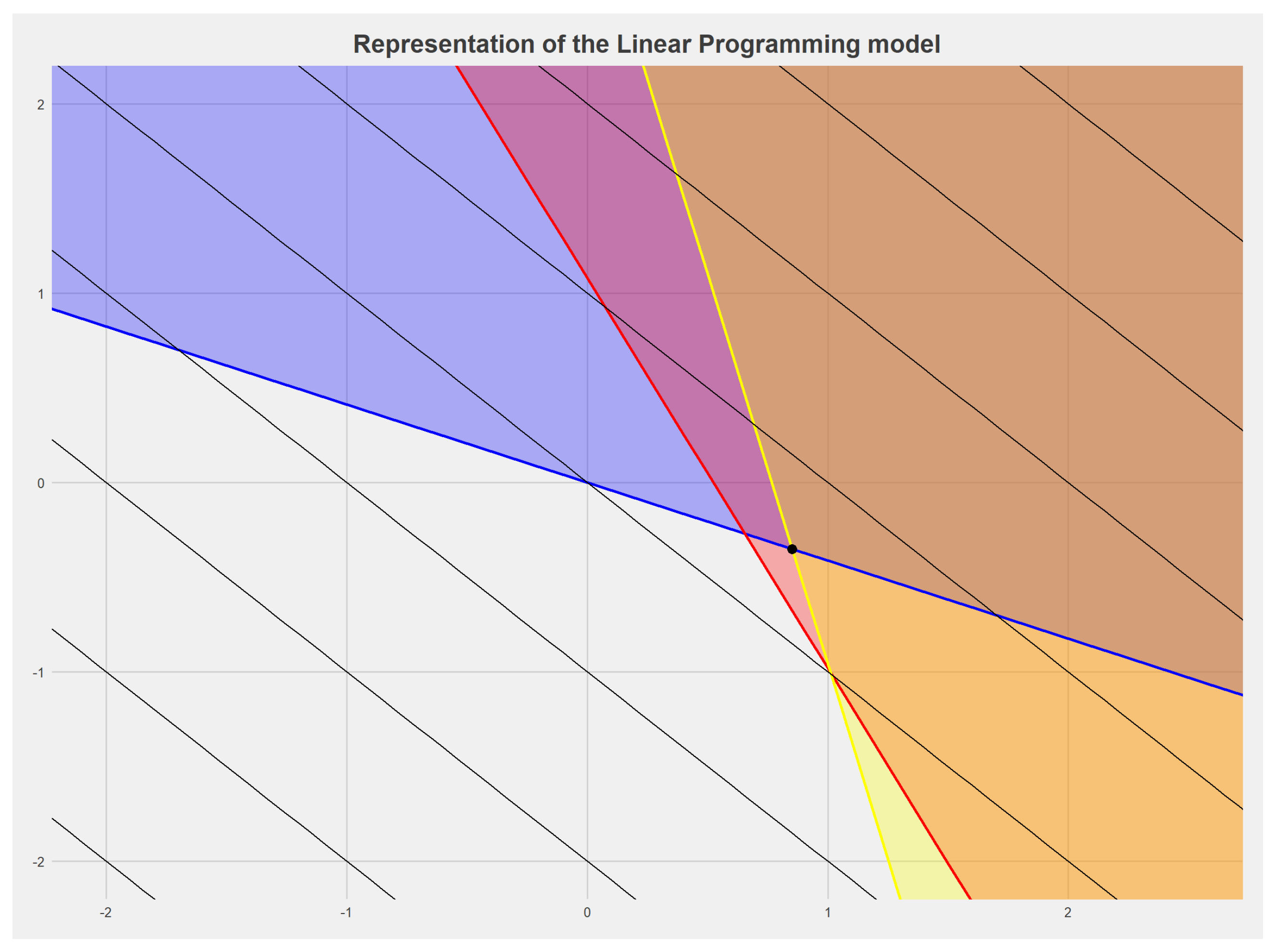
In Figure 1, we illustrate the problem outlined in Formula (42): specifically, the colored lines depict the boundaries of the three constraints (blue for the first equation, red for the second, and yellow for the third), while the shaded areas indicate the points satisfying their respective inequalities. The black lines represent the contour lines of the objective function to be minimized, and the black point represents the constrained minimum. This result can be easily obtained using any linear programming method, including contour lines or Lagrange multipliers.

The solution is ${\mathit{\theta }}^{*}=\left(0.8522,-0.3511\right)$ and the price of super-replicating portfolio is ${\mathcal{M}}_0·{\mathit{\theta }}^{*}=0.5011$ which coincides with the supremum of the non-arbitrage price range of the derivative.

An interesting aspect is that the vector ${\mathbf{Q}}^{*}$ linked to the ${\mathit{\theta }}^{*}$ strategy is

$${\mathbf{Q}}^{*}=\left(104/300,0,196/300\right)$$

(43)

As easily observable, $A_0=\frac{A_1·{\mathbf{Q}}^{*}}{(1+r)}$ and $S_0=\frac{S_1·{\mathbf{Q}}^{*}}{(1+r)}$, but at the same time, the second element of ${\mathbf{Q}}^{*}$ equals 0, making ${\mathbf{Q}}^{*}$ a martingale measure that is not equivalent to $\mathbb{P}$.

In

Table 2. Payoffs of the equity-linked policy vs. payoff of the super-replicating portfolio.

	${\mathit{A}}_1+\left[\mathit{max}({\mathit{g}}_1-{\mathit{A}}_1;0)\right]$	${\mathit{A}}_1+{\mathit{\theta }}_1^{*}·{\mathit{B}}_1+{\mathit{\theta }}_2^{*}·{\mathit{A}}_1$
${\omega }_1$	$250.00\%$	$250.00\%$
${\omega }_2$	$104.00\%$	$120.00\%$
${\omega }_3$	$104.00\%$	$104.00\%$

, we report the payoffs of the equity-linked policy and the payoffs guaranteed by the super-replicating portfolio: due to the incompleteness of the market, the insurer has set up a portfolio which, if state ${\omega }_2$ occurs where $S_1\left({\omega }_2\right)=1$, the portfolio not only obtains a performance that allows it to hedge the disbursements paid by policyholders, but it guarantees a profit of a strictly financial nature. From the insurer’s point of view, however, we observe that the policy has a high financial content. Given a unit investment, in only one scenario (${\omega }_1$), the insured sum receives a positive revaluation; in the other cases, however, the depreciation has a floor which makes the insurance operation less risky than the simple investment in the risky security. We now present the results of applying the simulation model. It is important to note that we simulated the profit/loss random variable 10 million times to ensure consistent and robust outcomes.

Regarding the real-world probabilities of the risky security values at time t = 1, we assumed a uniform distribution. This assumption primarily influences the magnitude of the model results but not the underlying logic.

Observing in line with the results previewed in Table 2, when the risky security takes on the values $S_1\left({\omega }_1\right)$ and $S_1\left({\omega }_3\right)$, the insurer’s portfolio is perfectly replicating, and the only source of uncertainty pertains to the mortality of the policyholders. On the other hand, if the risky security assumes the value $S_1\left({\omega }_2\right)$, the insurer’s portfolio ensures a positive profit regardless of the cohort’s mortality. This distinction underscores the impact of different scenarios on the insurer’s financial position, emphasizing the model’s versatility in capturing diverse outcomes based on the risky security’s behavior.

From the policyholder’s perspective, a crucial aspect concerns the real-world probabilities associated with the determinations of $S_1$. Notably, the purchase of a single policy unit ($P^{inv}=1$) entails an initial loaded premium of $\left(\lambda ·0.995·1.5011\right)$. Only if the risky security assumes the value S$\left({\omega }_1\right)$ does the final sum insured exceed the initial investment. It is essential to clarify that in the remaining two cases, any loss is mitigated due to the inclusion of financial guarantees provided by $i_{guar}$. From a purely financial standpoint, the policyholder has no incentive to buy the policy, as the price is too high, guaranteeing arbitrage to the insurer. However, the policyholder is averse to both financial and demographic risk and, for the latter, is willing to pay an additional price to cover, in this case, longevity risk. For the risk-averse policyholder, it is therefore possible to accept a policy whose derivative price is higher than the actual value, provided that the safety loading for demographic risk is lower than that required by other insurers who instead use the market’s EMM.

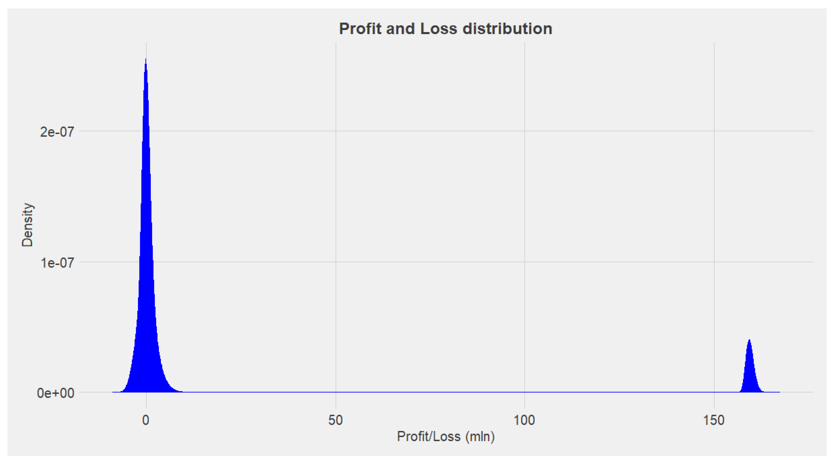
From the perspective of the insurer aiming to fully hedge against financial risk, losses are observed in both cases $S\left({\omega }_1\right)$ and $S\left({\omega }_3\right)$ when the observed survival is higher than expected. In insurance practice, it is common to quantify the implicit safety loading based on a ruin probability ranging from 30% to 50%. Setting $ϵ=30\%$, it is possible to calculate ${\lambda }^{Max}=1+0.01\%$. In Figure 2, we show the distribution of profit and loss obtained from 10 million simulations. We highlight that the loss in the worst-case scenario with a confidence level of 30% is around 700 thousand: from a computational standpoint, therefore, 700 thousand is the 30th percentile of the distribution of the aggregate benefits amount paid to the policyholders at time 1. With reference to Formulas (32) and (34), we observe that by using a first-order survival probability ${}_{1}p_x$ in the pricing phase equal to 0.996 (different from the second-order probability, considered realistic by the insurance company equal to 0.995), it is possible to request from the policyholders an additional aggregate premium exactly of 700 thousand monetary units such that the probability of ruin of the insurance company is exactly equal to the set $ϵ=30\%$. From a practical standpoint, therefore, the insurer aiming to fully hedge against financial risk will have to accept a greater probability of ruin $ϵ$ to compensate for the price difference between the market replicating portfolio (calculated under EMM) and the super-replicating portfolio.

Additionally, it should be noted that if the insurance company seeks economic results as independent as possible from financial scenarios, it can sell put portfolios, creating a so-called “reverse butterfly spread”. In this strategy, the insurer relinquishes profits derived from $S\left({\omega }_2\right)$ in exchange for a fixed amount. This approach allows for a more balanced and risk-mitigated financial position.

5. Conclusions

This study has delved into a discrete and incomplete market scenario, where the number of states surpasses the count of securities available. By breaking down the payoff structure of an equity-linked policy into components involving risky securities and financial derivatives, we established the infimum of the arbitrage prices of the derivative by minimizing the objective function tied to insurer costs. The incompleteness of the market ensures that the payoff of the equity-linked policy is not perfectly replicable, and any non-arbitrage strategy would result in financial losses in one or more scenarios. If the insurance company were to require complete immunization from financial risk, it could request the price of the super-replicating portfolio from the insured, provided it underprices demographic risk, accepting a higher probability of ruin. This approach presents two main avenues for improvement. Firstly, an effective strategy could be implemented to compute the derivative price under non-arbitrage assumptions and quantify financial losses. Secondly, the cost of capital could be further explored. Solvency II directive requires insurance companies to hold own funds necessary to cover annual losses in the worst-case scenario (Value-at-Risk measure) with a confidence level of $99.5\%$. The approach outlined in this paper allows for no financial risk (hence no capital requirement needs to be set aside) but entails higher demographic risk. This results in a greater allocation of funds for the latter risk. It is evident, therefore, that the calculation of the trade-off, absent in analytical form in this paper, could complement the discussion.