Abstract
This article provides both stylized facts and estimations of the endogenous nexus of the financial fragility hypothesis (FFH) with public social spending (PSS) for a paradigmatic Eurozone member country. The sample period 1995–2022 includes three major economic crises, the global financial crisis 2007–2009, the European debt crisis 2010–2015 and the COVID-19 pandemic one in 2020–2022. Within the context of the financialization literature, this paper is founded, for the first time, as far as we know, on the “financial fragility hypothesis”, combining the effects of both Minsky’s “financial instability”, as it has been extended for open economies, and the “Eurozone fragility one”. Similar to the relevant literature, the findings show that the PSS is associated, in a long-term steady state (cointegration), with the financial fragility process, starting, firstly, from the hedge-financing structure with high profitability of firms, when PSS decreases; secondly, to hyper-speculative financing with risky options, supported by bank credit and openness, indebtedness or discretionary fiscal policy, when PSS rises; thirdly, to the hyper-speculative or even Ponzi financing structures with over-indebtedness (leverage) from the global capital market, inflated asset prices and internationalized fragility, when PSS also rises, and so on. Our conclusion validates Minsky’s famous saying, “stability breeds instability”, also in the architecturally incomplete Eurozone. Policy implications are straightforward and discussed.
Keywords:
public social spending; financialization; Minsky’s extended financial instability hypothesis; Eurozone’s fragility hypothesis; animal spirits JEL Codes:
F36; F44; F62; G28; H12; H55; H63; I38
1. Introduction
Our neoclassical model of standard economics proves that it is not sufficient to simultaneous interpretation, on the one hand, the continuous transformation of economies and, on the other hand, the permanence of the market as a mode of production (Boyer 2022). The more resounding example is the global financial crisis of 2008 (GFC-2008). The fundamental three assumptions of this prevailing model, self-regulating and efficient markets, the rational behavior of actors and equilibrium, are obviously inadequate in explaining contemporary structural crises (Boyer and Saillard 2002). Today, we recognize the fact that the long-term dynamic development of the countries of East Asia was built on “proactive state policy” (Wade 1990). China’s resilience and better performance than North America after the GFC-2008 have shown that there may be more effective alternative development models (Boyer et al. 2011; Alary and Lafaye de Micheaux 2015). Especially in the European Union (EU), we should take into account that given complementarities among institutional forms, such as transfer payments and social security systems, the productive system and specialization imply more interdependence (not only competition), provided that a stable international regime prevails (Boyer 2022).
A crucial transformation of the contemporary Western economies (North America and Europe) concerns the institution of the “financial system”, which, in the last forty years or so, has gradually prevailed in almost all countries. More strictly speaking, this is the “financialization” phenomenon that shaped the transformation of countries’ growth models, e.g., the export-led, the welfare-led or even the consumption-led, to that of the finance-led growth regime (Boyer 2000). However, there is no unanimity yet for its definition. Mader et al. (2020) analytically explain a widely employed definition of the “financialization” offered by Epstein (2005), which is “the increasing roles of financial motives, financial markets, financial actors and financial institutions, in the operation of the domestic and international economies”. Alternatively, scholarship on financialization (van der Zwan 2014; Besedovsky 2018; Mader et al. 2020) has identified the following four different aspects: (1) the emergence of a new regime of accumulation, (2) the dominance of shareholder value, (3) the financialization of everyday life, and (4) structured finance and cultural as well as calculative transformation of credit rating agencies (CRAs). The literature on financialization can be classified into two groups depending on whether the focus of the research is microeconomic or macroeconomic (Cibils and Allami 2013). The last one includes economists from the following three schools of thought; first, “Régulation” (Boyer and Saillard 2002), second, “Post-Keynesian” (Minsky 1975, 1977, 1978, 1982, 1983, 1986, 1992a, 1992b, 1995, 1996), and third, “Radical” (Krippner 2005; Epstein 2005; Lapavitsas 2009).
The aim of this paper is to examine if the “financialization” of a European Monetary Union’s (EMU) member country (namely Greece1) can explain its public social spending (PSS) during the period 1995–2022. The famous welfare state, an element of the “identity” of the countries of the European Union (EU), is profoundly transformed2 in more and more financialized economies. Thus, in seeking relevant evidence, we investigate the research question “Is the financial fragility hypothesis (FFH) compatible with long run or steady state public social spending (PSS) of an EMU’s member-country (namely Greece), over the sample period 1995–2022?” The term FFH includes3 Minsky’s (1986) financial instability hypothesis (FIH) as it has been extended by Arestis and Glickman (2002) for open economies (eFIH) and the Eurozone fragility hypothesis (EZFH) (De Grauwe 2011, 2012, 2013; De Grauwe and Ji 2022), since Greece belongs to the core of the EU and that of the EMU.
To our knowledge, there is no other study to date that applies the FFH theory and our methodology. Moreover, the case of Greece as a small-open EMU economy is “paradigmatic“ because (a) it is internationally deficient, specialized mainly in services such as shipping or tourism, its financialization has been proven (Kyriakopoulos et al. 2022), while this literature is compatible with the endogenous “FFH-PSS” nexus we study here; (b) it was the only one of the EMU member countries for which the political system (Greece–EU) allowed the liquidity crisis of 2010 to slide into a solvency crisis and finally a sovereign default in 2012; it is the same country that, until the GFC-2008, had approximately the same credit rating by the CRAs as the other EMU member countries, but none of them (which experienced the Eurozone-sovereign or banking crisis, namely Italy, Portugal, Spain and Ireland) except Greece signed three MoUs4 with the Troika (IMF, European Commission and ECB5).
We focus on the theory of FFH as an appropriate stream of the financialization process transforming our economies based on the theoretical idea of endogenous financial instability or even crises, as well as because it seems that it satisfactorily interprets the PSS (Boyer 2013; De Grauwe 2013; Rossi 2013). The sample period 1995–2022 covers one and a half business cycles with three global or regional crises, the GFC-2008, the Eurozone debt crisis 2010–2015 and the economic crisis of COVID-19 pandemic (2020–2022). Eurozone fragility, always present over the sample period, is conceived on either issuing debt denominated in euro that member countries do not control or where no centralized fiscal budget exists, or even that the European Central Bank (ECB) cannot, by its statute, act as a lender of last resort for any country of the zone. That is why we have introduced a “Hyper-speculative” financing structure in order to take into account this permanent source of regional instability (EZFH).
The stylized facts we analyzed based on many time series graphs showed that the sample period could be divided into four sub-periods identified by the FFH as (a) the “super-speculative financing structure” 1995–2002, (b) a mix of “hedge and hyper-speculative financing structure” 2002–2008, (c) the “hyper-speculative financing structure” 2008–2018 and (d) the “hyper-speculative” but with some indications towards the “hedge-financing structure” 2018–2022. Furthermore, within this context, we provide consistent interpretations for the Greek PSS based on empirical models [ARDL (p, q1, …, qk)] estimated at long-term steady-state relationships (cointegrated) with the main factors of the FFH theory; under the limitation of Eurozone vulnerability, these could be allocated to the following stages: (a) clear profitability of the private sector; (b) its risky options supported by bank credits and discretionary fiscal policy; (c) openness to the global capital market and over-indebtedness, revealing “animal spirits” … until the produced instability leads to a new structure of markets restoring stability, and so on.
We contribute the relevant theory by providing the new term of “hyper-speculative financing” and the FFH economic interpretations of the public social spending of an EMU member country. The most important regional lesson resulting from the conclusion of this paper seems to has already been taken from the European authorities; for instance, one can see the reversal of the European monetary (PEPP6 by the European Central Bank (ECB) instead of OMT7) and fiscal (RRF8 by the European Commission instead of austerity) policies during the economic crisis of the COVID-19 pandemic (2020–2022) versus the Eurozone debt crisis (2010–2015).
Our research can be generalized to the Eurozone member countries. This is the goal for our next paper. Furthermore, the generalization question of this paper is equivalent to asking whether the Eurozone continues to be fragile. As De Grauwe and Ji (2022) explain, the ECB’s willingness to be the lender of last resort in member state bond markets is uncertain. President Draghi did so in 2012 with his famous “whatever it takes” and the OMT program, for which he did not have to put up a single euro. Will Lagarde or whichever next ECB president do so if need be? Since the problem Greece faced in 2010–2012 has not been institutionally solved, it could happen to any other member country of the EMU as long as bond holders, e.g., fund managers, fear (for any reason) that bonds will not be repaid at maturity, which could trigger a self-fulfilling liquidity crisis and even a default.
The structure of the paper is as follows. In the Section 2, we discuss the theoretical underpinnings of the financial fragility hypothesis, for which we document its explanation of public social spending or social security payments. In the Section 3, we describe the research design, modeling and the data analyzed in the paper. The Section 4 presents the empirical analysis and results with the relevant interpretations we offer, while the Section 5 concludes the paper.
2. Theoretical Foundation of the Financial Fragility Hypothesis
Public social spending (PSS) includes both demographic and economic categories of benefits. Demographic ones can be pensions or survivors’ and family support benefits, while those linked to the economic cycle can be sickness, disability, unemployment and social exclusion benefits. EMU members like Greece, as aging societies, are expected to have increasing needs for demographic categories anyway.
Economically, however, it should be stressed that, as Darby and Melitz (2008) have shown9, PSS for aspects like unemployment, age and health, and incapacity and sickness functions as an automatic stabilizer, i.e., their payments during recessions increase and conversely, in recovery, decrease. This evidence is very important because although PSS as an automatic stabilizer is proven to work in favor of a “smooth landing or take-off” of the economy, they do not seem to disprove the endogenous nature of cycles or even crises (as this paper also shows), as Minsky (1986) summarized in his famous phrase “stability breeds instability”. Thus, the automatic stabilizer argument enhances the respective of the introduction section that this paper’s evidence could be generalized in the Eurozone.
Thus, as transfer payments are recorded in government expenditures, PSS follows the mechanism of income redistribution (social policy) within the effectiveness of fiscal policy. More specifically, the European System of Accounts (ESA 2010, § 4.83) defines the (PSS) “Social contributions and benefits (D.6) as: social benefits are transfers to households, in cash or in kind, intended to relieve them from the financial burden of a number of risks or needs10 [(a) sickness; (b) invalidity, disability; (c) occupational accident or disease; (d) old age; (e) survivors; (f) maternity; (g) family; (h) promotion of employment; (i) unemployment; (j) housing; (k) education; (l) general neediness], made through collectively organized schemes, or outside such schemes by government units and Nonprofit Institutions Serving Households (NPISHs); they include payments from general government to producers which individually benefit households and which are made in the context of social risks or needs”.
In order to develop our research question, we start with the broad theoretical body of “financialization”, which has been recently excellently overviewed by Mader et al. (2020). We can distinguish the economists who work at a microeconomic level from those who are interested in the great picture or the macroeconomy. The latter include the Regulationist (Boyer and Saillard 2002; Boyer 2000, 2022), the post-Keynesian (Palley 2007) and the Radical (Krippner 2005; Epstein 2005; Lapavitsas 2009) schools of thought. Among post-Keynesians, the financial instability hypothesis (FIH) theory proposed by Minsky (1957, 1975, 1982, 1986) holds a dominant position in the literature because of its great interpretative capacity for business cycles and crises, like the GFC-2008 or the Eurozone’s (2010–2018) one.
Minsky introduced the term “money manager capitalism” to describe not only a version of capitalism that is dominated by financial motives and activities but rather to define capitalism as financialized by default (Sotiropoulos and Hillig 2020; Christophers and Fine 2020). In this perspective, his FIH is founded on the idea that any (capitalist) economy endogenously establishes a financial structure which is susceptible to crises (Minsky 1983). Its economic performance is mainly determined by the way firms finance their fixed capital investments. Thus, in the first stage of the upward trend of a business cycle, often called the “recovery phase”, economic actors (primarily the businesses) are able to finance from their operations both the interests and principal of their loans; Minsky called this financial structure “hedge finance”. The reason seems to be that both lenders and borrowers do remember recent depression times, so they behave conservatively, while investment plans are mainly financed by internal sources (retained earnings) rather than through banks or other external sources. So, corporate “profitability” seems to be not only the starting point for the hedge financing stage but also its foundation, due to the fact that the previous period of high risk is still “alive”.
Nevertheless, “A break in the boom occurs whenever… reversals in present-value relations take place. Often this occurs after the increase in demand financed by speculative finance has raised interest rates, wages of labor, and prices of material so that profit margins and thus the ability to validate the past has eroded” (Minsky 1986, p. 220). Arestis and Glickman (2002) underline here what is the most important, which is in contrast with the neo-classical model, though strongly compatible with financial (in origin) crises, i.e., the endogenous nature of the events that break the boom reached by the economy. Although Minsky (1977) accepts that the catalyst of a crisis could be an “external” event, he steadily denies the “exogenous shocks or accidents or even policy errors”, writing that “our economy endogenously develops fragile or crisis-prone financial structures” (Minsky 1977, pp. 139–40). Thus, the memories fade due to the increased output (fueled by raised investments), which causes optimism to prevail in markets. This triggers entrepreneurs (see, Schumpeter’s sense) to promote projects on innovative products, which inevitably come, this time, with more risky debts. Hence, some of these risky investments could fail (due to the mentioned reversal of present values caused by raised income, interest rate and so on), while if the failures last, then the respective borrowers could not be able to repay (at least) part of their loan. If the bank still believes in the project, it may refinance the principal while it steadily receives interest. Minsky calls this second stage of the FIH “speculative” finance. External financing and growing debts characterize the speculative financing stage. The duration of this speculative financing stage could be prolonged by reckless leveraging, which actually could be translated as the exposure to risk of asset prices’ collapse (Dow 2020). Thus, in Minsky’s thought, financial leverage, increasing the ratio of debts in the capital structure, is really significant for the liquidity, the solvency and finally the bankruptcy of any agent.
When a “market” is witnessed of a number of insolvent borrowers, or if it happens that a policy is reversed by the authorities, then firms, sectors or even the economy as a whole could enter the final (third) stage of the Minskyan FIH, that of “Ponzi” finance. In the latter, the borrower can repay neither the capital nor the interests of their debts from operational cash flows; thus, they are bankrupted.
The direct consequence of the FIH is the famous Minskyan quote “stability breeds instability” over the long term, because of the endogenous devaluing of liquidity, the easy lending standards by the deregulated banking system, and the ensuing private debt—leverage—in order to support inflated asset values and the rising expensive capital stock (Holloway and Eloranta 2014; De Grauwe 2013).
In addition, innovation could also come from credit institutions, as happens in reality. This concerns their well-structured processes and their financial products: first, the worldwide deregulation process, starting in the early mid-70s from the US, which mainly gave birth to the globalization process (Sen 2020); second, the liberation of international financial transactions, notably free and easy capital flows (after the collapse of the Bretton Woods system in 1973); third, crucial financial innovation instruments, i.e., mainly derivatives, like forward, futures, options, and swaps originating from commodity markets or even collateralized debt obligations (CDO) or mortgage- (or asset-) backed securities (MBS or ABS) or credit default swaps (CDS) and the like; it is noteworthy that when financial assets are not backed by physical ones, then they constitute the essential components of an aspect of the financialization process (Blanchard et al. 2021). We refer in summary to the capabilities offered by all these processes and instruments as “the drive towards financial innovation”. The latter is explained in detail by Arestis and Glickman (2002) who extended the Minskyan FIH (eFIH) in order to show the state of the internationalized financial fragility, whereby an economy could fall when, in addition, domestic agents borrow in foreign exchange. They distinguish three (3) potential scenarios: (i) a crisis that is domestic (d) in origin but impacts its external (e) situation (they give this the term “d to e crisis”); (ii) a crisis that is external (e) in origin but impacts its domestic (d) situation (they give this the term “e to d crisis”); and (iii) crisis-intensifying interactions between (i) and (ii).
The first (i) potential scenario, a “d to e crisis”, as already mentioned, starts from a rising cost of domestic capital goods, while, as Minsky argues, the result will be present-value reversal and a decline in asset prices. However, the speculative financed units in the closed economy of the early Minskyan analysis are transformed now into the open one to “super-speculative” finance because of the huge outflows of international portfolio investments (both by non-residents and residents) who cannot afford the devaluation of their domestic assets. The latter causes the home currency to devalue too, or it could even trigger an exchange rate crisis. Thus, domestic firms in the open economy are now vulnerable due to the fact that even if they were hedge-financed in the beginning (matching asset and liability maturities), they have incurred debts in foreign exchange, while their cash flows are denominated in the home currency. The contagion effects could now be internationalized. As regards the openness of the country to global financial markets, this could cause the second (ii) scenario, a “e to d crisis”, through the foreign exchange market or the form of its international integration, e.g., it could be a member of a monetary union (e.g., EMU). So, in the stand-alone case, the residents could accumulate debts denominated in foreign currencies; as long as the central bank can also increase the official reserves so as to be able to finance the relevant liabilities with no need for intervention in the foreign exchange market, then hedge-financing could be sustainable; however, when the endogenous process drives up the debt-to-reserves ratio (especially short-term debt), creating doubts regarding the ability of monetary authorities to preserve the purchasing power of the home currency, then the market expectations for the exchange rate could become a source of uncertainty, destabilizing the domestic economy vs. the rest of the world; thus, possible fire-sales of the home currency could, in effect, downgrade the finance of domestic units, including that of the state, to the so called super-speculative (Arestis and Glickman 2002) or even the Ponzi financing final stage (equivalent to bankruptcy). The external finance of Minsky’s speculative stage is now exacerbated by foreign exchange markets’ effects, hence the term “super”-speculative.
Furthermore, in the case of the member countries of an incomplete monetary union like the Eurozone (or EMU), the super-speculative stage can become even worse. This is because they have delegated their monetary policy to the ECB, which, by its mandate, cannot act as a lender-of-last-resort, and hence, the members of the EMU cannot give a 100% guarantee to their bondholders that they will have the necessary liquidity to pay them out at maturity (Boyer 2013; De Grauwe 2013; Rossi 2013; De Grauwe and Ji 2022). Put differently, Greece, like every member country of the EMU, issues government bonds in the home currency, the euro, over which it has no control. Thus, as has historically been confirmed, after the GFC-2008 and the ensuing Eurozone sovereign debt crisis that erupted in 2010 (EZ-2010), the unified till then bonds’ risk was priced differently since then by the relevant capital market for the South and West Euro-Area Periphery countries (SWEAP) than for the core ones (CORE). This special risk that a government of an EMU member state can run out of cash, which creates the potential for self-fulfilling liquidity crises that may force it to default (as it was the case for Greece in 2010–2012), cannot arise in standalone countries because the central bank of the latter can issue whatever amount in home currency to repay its government bondholders at maturity. Thus, in order to take into account this additional Eurozone-country risk to the super-speculative scheme of Arestis and Glickman (2002), we introduce the term “hyper-speculative” financing units, so as to complete the financial fragility hypothesis (FFH). The latter is theoretically expected to affect the EMU’s government expenditures of the sample era, part of which are the (Greek) PSS we analyze in this paper.
It is worth noting that this aforementioned risk fragmentation of the EZ-2010 (coming from the diversity of the government bond yields, distinguished into bad and good clusters) and the ensuing burst of the Eurozone’s fragility11 did not happen during the economic crisis of the COVID-19 pandemic, and thus did not trigger a new sovereign crisis. The reason was probably the monetary (the unconditional PEPP of the ECB) and fiscal (the first “Eurobonds”—NGEU12 program) policies applied by the European authorities (De Grauwe and Ji 2022).
In Figure 1, the main factors of the FFH affecting PSS are schematically allocated to the following three stages:
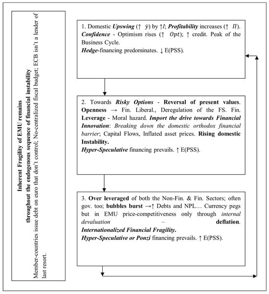
Figure 1.
Financial fragility hypothesis (FFH): an endogenous process. Notes: = real gross domestic product (GDP) growth; I = business (fixed) investments; E(PSS) = theoretically expected value of public social spending (PSS) or social security payments; = profitability; = optimism; EMU = European Monetary Union or Eurozone (EZN) member countries; FS = financial system; ECB = European Central Bank; NPL = non-performing loans.
- (a)
- Starting from “stability economic conditions”, the domestic results mainly increase the profitability of the private sector. “Hedge financing structure” prevails. In general, PSS is expected to decrease as output raises [↓ E(PSS)].
- (b)
- The entrance of new foreign direct investments (FDIs) or even short-run portfolios increase risky options for domestic small-medium enterprises (SMEs), which seek bank credits and discretionary fiscal policy resulting in financial leverage—indebtedness—while the inflated asset prices and exposure to foreign funds feed instability conditions of “hyper-speculative financing structure”. In general, PSS is expected to increase as output is squeezed [↑ E(PSS)].
- (c)
- The “animal spirits” of the financial downturn should be “paid” by the government through austerity policies… “Ponzi-finance” is exacerbated by the Eurozone’s inherent fragility. In general, PSS is expected to increase as output is squeezed [↑ E(PSS)]. New markets’ structures give birth to a new round from stability to instability, and so on.
Based on the aforementioned theoretical analysis of FFH (Minsky 1986; Arestis and Glickman 2002; De Grauwe 2011; Mader et al. 2020), it is considered plausible to empirically investigate the following research question: “Is the financial fragility hypothesis (FFH) compatible with long run or steady state public social spending (PSS) of an EMU’s member-country (namely Greece), over the sample period 1995–2022?”
Kyriakopoulos et al. (2022) provided theoretical support and empirical evidence for the financialization of the Greek economy based on Boyer’s (2000) seminal paper. They confirmed the compatibility of a number of mechanisms that originated from the financial system (see Boyer 2000, Figure 3) and impacted the dependent variable of PSS. However, in this paper, we have proceeded a step further: we elaborate on the specific theoretical underpinnings of the FFH theory in this section; we appropriately apply, in the following section, the ARDL (p, q) econometric method of Pesaran et al. (2001); and finally, we propose the variable selections tailored to explore the endogenous impacts of financial instability on PSS.
3. Research Design, Modeling and Data
The epistemological problem of the difference between research data and research purpose, is also present in this study, where our effort is to identify if the whole economy or a sector is in a specific Minsky financial stage. However, we can obtain a wider picture, as for instance, when during the Eurozone sovereign debt crisis in 2010–2012, the bond market sentiments transformed the Greek government’s liquidity crisis to a solvency one and eventually forced it into bankruptcy; this obviously constitutes the Ponzi finance stage. In addition, we would be making an epistemological error if we tried to “prove” our falsifiable research question (Popper 2002; Kuhn 1962; Hepburn and Andersen 2021). We only try to test if the FFH could be considered compatible with the long term or steady state of an EMU’s member country (Greece) PSS (cointegrated) over the sample period 1995–2022.
As explained earlier, the financial fragility of a small open Eurozone-member economy arises when endogenous factors predicted by the theory appear and cause either ups and downs of business cycles or, even worse, crises. Thus, we develop a double test for the relationship, “FFH, the cause—PSS, the effect-purpose”; first, we use descriptive statistics with many time series graphs in order to see if the stylized facts of the Greek economy’s impacts on PSS tell the story of the FFH; second, in the econometric analysis, we identify autoregressive distributed lag [ARDL (p, q1, …, qk)] empirical models so as to test if there are long-run (cointegrated) relationships between the dependent of the PSS and a number of “independent” variables expressing the factors predicted by the FFH theory.
More specifically, the social contributions and benefits (D.6) paid (PSS) in Greece include13 seven out of twelve risks or needs provided by the (ESA 2010), that is, (1) old age (pensions), (2) sickness, (3) survivors, (4) disability, (5) family, (6) unemployment, and since 2014, (7) social exclusion14 (see Appendix A, Figure A13 evolution of the PSS composition).
We expect that the main factors of the FFH affecting PSS, as they have been explained in the previous section and presented in Figure 1, can be detected from estimations of our empirical ARDL (p, q) models. However, a limited effect of PSS functioning as an automatic stabilizer is expected, especially during the period of the Eurozone debt crisis (2010–2015), not only because of the Stability and Growth Pact (SGP of the EMU) predictions15 still in place, but mainly because of the harsh austerity–deflation policies imposed on the country by the Troika (International Monetary Fund—IMF, European Commission—EC, and ECB) through the memoranda (MoU) signed by the government. They treated PSS as a luxury good with low-income elasticity.
So, first, we investigate whether the “profitability” of sectors or the economy as a whole is such that the constant expansion of the real output can be justified, i.e., whether we can detect the “stability conditions” expressing “hedge finance”. If the data (primarily of the non-financial sector) record a sharp increase in credit and then loans with a parallel increase in asset prices, this could suggest a robust financial structure in that period (hedge finance). Conversely, if endogenous forces push asset prices down, while private sector borrowing increases, alongside anemic growth in real output (a widening output gap), then our open Eurozone-member economy slides into a “hyper-speculative financial” structure. Hence, this could reflect an advanced stage of the Minsky moment “stability breeds instability”. Further, for Greece, which belongs to the EMU, the previously mentioned Eurozone fragility factor should be added. That cumulative effect of “free capital movements plus the membership of the incomplete EMU”, we have called the “hyper-speculative” financial structure. Finally, the “Ponzi” finance stage can be easily ascertained from declared solvency crisis—defaulting.
We specify the long-term model in Equation (1).
where = Greek social contributions and benefits paid (the dependent variable); = 1, …, k explanatory variables; t = time in quarters; = the disturbance term.
By implementing the Pesaran et al. (2001) bounds testing approach for the cointegration, and by rewriting Equation (1) in an error-correction model (ECM) form, the short-run effects of the FFH factors on PSS are presented in the Equation (2) (Hajilee et al. 2021).
To demonstrate the long-term relationship, we need to control two criteria, namely the sign and significance level of the error-correction coefficient (); a significant negative is an indication of a long-term relationship or cointegration among the variables.
Equation (2) has been estimated in five (5) different models according to the FFH structure summarized in Figure 1, while estimations of the variables are presented in Table 3. The definitions and sources of the variables are reported in Table A1 of Appendix A. So, the vectors of independents include Model 1, focusing on the “profitability factor” = (invgdp, realgdp10yy, discrpol, goss11gdp, goss12gdp); Model 2a, focusing on the “risky options and financial development factors” = (realgdp10yy, discrpol, credtnfgdp16, credtfgdp); Model 2b, focusing on the “Openness and indebtness -leverage” = (realgdp10yy, discrpol, cagdp, s11debtgdp, pudbtgr, s1ltloanss2tot); Model 2c, stressing the “Inflated asset prices and foreign funds exposure” = (realgdp10yy, cagdp, s11debtgdp, s1ltloanss2tot, hpiyoy, asegspiyoy, gr10ygby); and Model 3, focusing on “Animal spirits “paid” by the gov.” = (discrpol, m3outsgdp, nlbs13gdp, rgsnowb).
An example of the analytical form of Model 1 (Table 3) as a special case of Equation (2) is presented in Equation (2a).
As Kyriakopoulos et al. (2022) mentioned, the Pesaran et al. (2001) estimation approach used in this paper has three main advantages over other methods of cointegration: it obviates the unit root pretests to identify the degree of integration of the time series; it can be used with either I(0) or I(1) variables, but not I(2); a one-step simultaneous estimation on both long-term and short-term models is applied. The procedure involves three stages (Goel et al. 2008): first, searching the long-term (level) relationship among the variables applying the bound tests through the estimation of a conditional ECM; second, the lagged dependent-variable term and the one-period lag on regressors are tested for joint significance via an F-test, under the (null) H0 “variables have not relation in levels” and using the critical values of Pesaran et al. (2001), and a supplementary t-test is available for the significance of the lagged dependent variable, with critical values again provided by Pesaran et al. (2001); third, if from the previous tests a level relationship cannot be rejected, then the long-term or cointegrated one is estimated through the ARDL procedure, as proposed by Pesaran and Shin (1999).
In Table 3, only the estimated coefficients ( and ) of the ECM are presented, since we are interested only in long-term cointegrated relationships.
As regards the “discretionary fiscal policy” variable (discrpol), this was based on the methodology of Fatás and Mihov (2003), and we have used it as a proxy of the unobserved government expenditures such as the “interest paid for the public debt” or “countercyclical additional payments”. It comes from the residuals of the ordinary least squares (OLS), estimated using Equation (3)
where is the growth rate (yoy) of the government consumption expenditures; is the growth rate of the nominal gross domestic product (GDP); is the inflation rate as measured by the general consumer price index; is the squared inflation; is the growth rate of fuel price index (yoy).
4. Empirical Analysis and Discussion
We begin with a wider picture of the economy 1995–2023 based on the raw variables and stylized facts shown in the graphs provided in Appendix A. It should be pointed out that although PSS payments are transfer payments, they are nevertheless recorded in government expenditures and hence in the state budget; see fiscal policy.
So, in the first step of (descriptive statistical) empirical analysis, one can find out if the national accounts data, which we processed and present in Figure A1, Figure A2, Figure A3, Figure A4, Figure A5, Figure A6, Figure A7, Figure A8, Figure A9, Figure A10, Figure A11, Figure A12 and Figure A13 in Appendix A, are compatible with the FFH as summarized schematically in Figure 1. From the latter arise the turning points one looks for: (a) profitability feeding a climate of confidence–optimism and rising credits, which could express the Minsky “hedge financing” stage; (b) a sequence from the undertaking of risky business investment plans with extra leverage in foreign exchange currency and the reversal of present values with shrinking profit margins, to a rise in outstanding debts and pessimism and capital outflows with likely liquidity crisis, which could be translated as the “hyper-speculative financing” stage; (c) according to the finance-led growth regime adopted as part of the insertion of the country into the incomplete EMU (Kyriakopoulos et al. 2022), this choice could also lead to bankruptcy, or, in Minskyan terms, to a “Ponzi financing” structure.
We think that the accumulative information of the facts reported in Figure A1, Figure A2, Figure A3, Figure A4, Figure A5, Figure A6, Figure A7, Figure A8, Figure A9, Figure A10, Figure A11, Figure A12 and Figure A13 of Appendix A need not be explained. A few comments could be useful:
Given that we are interested in (endogenous) financial instability, the starting point should be the overall performance of the economy recorded by the history of the GDP (see Figure A2). The global financial crisis of 2008 (GFC-2008) and the Eurozone debt crisis 2010–2014 had a decisive structural impact on the economy, which is reflected in the large decline in employment in manufacturing (≃32%) over the 2008–2014 recession and its stagnation since then, while the respective approximately constant increase in the financial sector is reflected in a jump in their ratio of FI/MNF (see Figure A1). The profitabilities, measured by the gross operating surplus19 to GDP, of the non-financial sector (↓18%) and financial sector (↑67%) follow opposite tendencies and translate the increase in the financialization of the economy as well as the transition from a hedge–financial structure to a hyper-speculative one (Figure A2 and Figure A3).
The snowball effect shown in Figure A11 can express the change in the climate of confidence from euphoria during 1995–2008 to pessimism or animal spirits over the deep recession 2008–2014, stagnation 2014–2018 and some recovery since then. The most important structural damage in a long-term perspective is demonstrated in the de-investment of the economy (see Figure A6 and Figure A8). In financial terms, the reversal in profit margins (2008–2014) can be confirmed by respective asset price falls (dwellings, the stocks in the Athens exchange and government bonds) (see Figure A4, Figure A5 and Figure A9). The hyper-speculative financing structure can once again be detected.
The international investment position (BP-IIP20) of the country is steadily negative and in fact continuously deteriorated over the 2002–2022 period (see Figure A12). The stylized facts of the international borrowing of the country are compatible with the FFH and are similar to those in the literature (Vigny 2022; Amoutzias 2019).
The facts could be interpreted as showing a de facto “Ponzi financing structure”, as the productive private sector (S.11) was obliged to work with no credit since 2014 while outstanding debt accumulated (see Figure A6, Figure A7 and Figure A8). Regarding the overall performance of institutional sectors [(non-financial (S.11), financial (S.12), government (S.13) and Households and NPISH (S1.M), and the domestic economy (S.1)] can be approximated by the measurement of “net lending (+ surplus)/borrowing21 (- deficit)”22 to GDP (Figure A10).
Thus, in Minskyan terms and based on Table 1, it seems23 that respective data are compatible with a “speculative” financial structure during the period before the introduction of the euro (1995–2002); then, the structure was “hyper-speculative” (2002–2012); after that, the “Ponzi-financing” structure dominated since the government defaulted and bank recapitalized in 2012 till 2015. From 2016, there was a return to a recovery trend with “hyper-speculative financing”, because, despite the change in European policies (see PEPP and RRF at least), Eurozone fragility remains (De Grauwe and Ji 2022).

Table 1.
Indications from our sample for the Minskyan financial structures (averages of periods).
In the second step of the empirical analysis, we provide econometric estimations (Table 3) and interpretations compatible with the FFH. The social contributions and benefits paid as a ratio of GDP (scbtotgdp) are explicitly defined as the dependent variable of the estimated empirical models identified in ECM forms as presented by Equation (2) or (2a). In Table 2, the summary statistics of the variables used in the ARDL (p, q) estimations are shown. The availability of data has defined their time span as well, so that we do not have a balanced time series sample.
Table 2.
Summary statistics of the variables used in ARDL (p, q) estimations.
In the estimated models27 presented in Table 3, it was not possible to distinguish sub-periods of the business cycle detected in the previous descriptive analysis, for econometric reasons, due to the insufficient data in the demanding process of ARDL (p, q) co-integration relations. We should start the evaluation from the “Diagnostic Statistics, Pesaran et al. (2001) bounds tests and Adjustment EC-Term”. Both the F-test and t-test confirm the existence of a cointegration relationship for all the five models; this is equivalent to saying that our research question cannot be rejected (at 1% significance level) given the second condition of the negative sign and strong significance of the estimated coefficients of the ECM; the latter vary between −0.76 and −1.51, indicating fast and very fast adjustment of the system. That is, between 76% and 151% of the total difference from the short-run dynamics to the long-term equilibrium trend was occurring within the coming quarter of the sample period. Based on the remaining diagnostic tests, the estimated models cannot be rejected.
Table 3.
ARDL estimations.
Model 1 (see Table 3) provides statistically significant estimations for the factors concerning “profitability”, private investments, growth and discretionary fiscal policy (see also Figure 1, stage 1 seems to prevail here), which are proved to be in a long-term steady state with the dependent of the “social contributions and benefits to the GDP” (hereafter PSS). Thus, when the gross operating surplus of the non-financial sector and the financial one (as a proxy of the “profitability” of these main sectors of the economy) rise, the PSS decreases29 because the increasing output, income and employment reduce the need for social support, mainly for old age, sickness and survivors30 (↑goss11(12)gdp → ↓scbtotgdp). The same reasoning for the rising efficiency of the economy can also be used to justify the even more statistically significant (at less than 0.001 level) negative relationship of both private investments and the growth rate of the economy with the dependent of the PSS [↑(invgdp, realgdpyy) → ↓scbtotgdp]; see relevant Figure A1, Figure A2, Figure A3, Figure A4, Figure A10 and Figure A13 in Appendix A. These findings are in line with Pierros (2020). The opposite statistically significant positive steady state relationship between “discretionary policy” and PSS can be justified by the government expenditure that does not concern either permanent behavior, nor the increase in economic activity, nor inflation or fuel subsidies31, but rather and probably the electoral cycle or populist extraordinary benefits, etc. (↑discrpol → ↑scbtotgdp).
In Model 2, we focused on the explanatory variables concerning risky options—financial development, openness and indebtedness—leverage of the economy (see also Figure 1, stage 2 seems to prevail here). Credits can increase the corporate turnover, which is associated with employees’ increased sickness or invalidity or occupational accident and disease, as well as greater requirements for supporting maternity and family, housing or education from the social security system; hence, there is a positive estimated coefficient for the relationship between “credits to the non-financial sector” and PSS (Model 2a) (↑credtnfgdp → ↑scbtotgdp). Also, the higher the credits to households, the more the family can be expected to grow, and that is why, for the majority of employees or workers (middle or lower incomes), more PSS is needed for housing, education, health and so on; this can be a reasonable interpretation of the positive relationship with the PSS estimated in Model 2a (↑credthgdp → ↑scbtotgdp); see relevant Figure A6 in Appendix A. These findings are also similar to those of Amoutzias (2019).
Rising current account balances or a shrinking deficit, and an implicit increase in the international competitiveness of domestic production, translates a respective increase in net private investments, while both factors cause GDP growth (↑cagdp → ↓scbtotgdp); the latter, as explained earlier, is negatively related to the automatic stabilizer PSS; see relevant Figure A12 in Appendix A for the international investment position of the country (BP-IIP). Furthermore, the outstanding debt of the non-financial sector (S.11), which has been estimated to be positively related to PSS, can pass, in good times (see the 1995–2008 period here), the threshold of heavy financial leverage, which, in turn, refers to the transition from the Minskyan “hedge to hyper-speculative financing”. To put it differently, the excessive growth of private debt in times of euphoria, with an increase in the cost of capital (and the lack of capital goods produced by domestic manufacturing32), due to its equally excessive demand, since it reverses present values, leads to corporate bankruptcies. Thus, it causes a decrease in production, income and employment, and therefore, there is a strong need to increase social support for the affected (i.e., raise of the PSS); hence, there is a positive and strongly significant estimated relation “outstanding debt of the non-financial sector—PSS” in Models 2b and 2c (↑s11debtgdp → ↑scbtotgdp); see relevant Figure A8 in Appendix A.
However, the growth rate of public debt is not a surprise that is estimated to negatively affect PSS because it focuses on the rate of increase and not on the level of this debt. So, because this factor is perceived as synonymous with the fear or even the panic of the capital markets, to whose rising they react with fire-sales of bonds or other assets to push up their yields, real interest rates and so on, provoking once again the reversal of present values, investment failures and bankruptcies. This process ends in a recession that demands governments to release (or at least not brake or restrain) automatic stabilizers like PSS in order to support the affected. Of course, this process in the Greek case was much worse because the Troika imposed deflation policies—austerity—although they found a liquidity crisis in the onset at 2010 and not a solvency crisis! The deflation process blocked the operation of PSS—automatic stabilizers (↑pudbtgr → ↓scbtotgdp)! These began to operate in a limited and gradual manner after 2012 and Draghi’s “whatever it takes”, the restructuring programme (PSI), and the change in the composition of public debt from bonds to mortgage loans from the Eurozone member countries through the ESM; see relevant Figure A9 in Appendix A. So, in practice, it seems that the monetary policy determines the sustainability of the public debt, as is predicted by post-Keynesians.
The variable concerning the long-term borrowing of the non-financial sector (S.11) from abroad as a ratio to the total of its corresponding loans (Models 2b, 2c) is also of paramount importance. A statistically significant positive (cointegration) relationship with PSS was estimated. Its interpretation is similar to that of the outstanding debt of the sector, but here, it is not enough to add the risk of the foreign currency. We should also add that of the Eurozone’s fragility hypothesis (De Grauwe 2011). That is why we propose to expand the Arestis and Glickman (2002) term of “super-speculative” with that of “hyper-speculative” in order to also include the risk that the EMU financing units issue their debts on the euro that no country controls (↑s1ltloanss2tot → ↑scbtotgdp); see relevant Figure A12 in Appendix A.
The estimated long-term relationship between asset prices (housing, stock prices—general price index, as well as 10-year government bond yield) and PSS theoretically only has an expected positive sign for the last one, the yield of 10-year government bonds (Model 2c). When this yield rises, it translates the decrease in the price of traded bonds due to some kind of fear. Domestic interest rates are gradually influenced upwards, which reduces aggregate demand, output, income and employment. To the extent that public social spending (PSS) acts as an automatic stabilizer, it will increase as estimated in Model 2c [↑gr10ygby → ↑scbtotgdp]. As regards housing prices and prices of the Athens stock exchange, the estimated positive cointegrated relation could be explained like this: in times of crises (GFC-2008, EZ 2010–2015, COVID-19 2020–2022), the restructuring of the goods–services market due to bankruptcies or M&As33 of firms (usually small and medium-sized enterprises34) generally increases the profit margins (determined independently of unemployment) of the survived, while labor wages decrease due to the large increase in unemployment caused by the recession35. Then, logically, automatic stabilizers such as PSS work in the opposite way, and therefore, there is a positive correlation between asset prices (especially equity prices) and social spending on relief for the affected [↑ (hpiyoy, asegspiyoy) → ↑scbtotgdp]; see relevant Figure A4 and Figure A5 in Appendix A.
Finally, in Model 3, we present estimations concerning indicative monetary and fiscal policy measures reacting to over-leverage and internationalized financial fragility. It should be noted that regardless of the investment grade given by the CRAs36 for Greek government bonds (junk until 2023), the ECB bought them (“waiver”) for reasons of financial stability of the Eurozone; the latter caused a credit boom from the financial sector of the core EMU countries towards Greece as a result of the increase in its private debt (especially due to a real estate boom; see Figure A1, Figure A6, Figure A7 and Figure A8 in the Appendix A) up to the GFC-2008 (Boyer 2013). Thus, the expansionary monetary policy (M3/GDP) of the ECB through Keynesian short-term processes drives lower interest rates and higher outputs, whereby income and employment are compatible with less need for PSS. However, as prices rise due to excess aggregate demand, in the long term, real money balances fall, interest rates increase with output, and incomes and employment decrease; hence, there is a rise in automatic stabilizers of PSS, such as employment promotion policies (↑m3outsgdp → ↑scbtotgdp). This evidence is similar to that in Rossi (2013). The snowball effect (r-g) has been estimated as a positive steady-state relationship with PSS; when it rises, the public debt rises too, while contractionary effects result in a lower output, income and employment, causing an increase in PSS (↑rgsnowb → ↑scbtotgdp). In the end, the increase in net government lending (+) (i.e., the primary fiscal budget surpluses, not only from the austerity policies implemented in crises but also due to the SGP of the EMU before them) ameliorates the mood in the markets, causing a decrease in interest rates and a respective increase in profit margins (especially if public property is sold as it was here—a condition of the Troika lenders) and so on as aforementioned; hence, lower amounts of PSS are needed, justifying the estimated negative relationship (↑nlbs13gdp → ↓scbtotgdp); see relevant Figure A10 and Figure A11 in Appendix A.
The findings reported in Table 3 are in line with the financialization literature, particularly with the FFH, including the incomplete Eurozone architecture and asymmetric governance (among others, Vigny 2022; De Grauwe and Ji 2022; Pierros 2020; Amoutzias 2019; Boyer 2013; Rossi 2013).
5. Conclusions
In this paper, we have investigated the research question “Is the financial fragility hypothesis (FFH) compatible with the long-term or steady-state public social spending (PSS) of an EMU member country during the period 1995–2022?” Based on stylized facts and relevant econometric estimations, we have reported (for Greek data) that we could not disprove it. Methodologically, transfers of PSS are included (ESA 2010) in government consumption, so they have to be treated as part of the general framework of the fiscal policy. The latter require that we analyze the whole economic system, within the limitations of the Eurozone’s fragility, and referring to the FFH, as endogenously breeding instability and activating the automatic stabilizers like PSS.
Within this context, we provided interpretations for PSS, which was estimated [with ARDL (p, q)] to be in long-term steady-state relationships with the main factors of the FFH schematically and comprehensively presented in Figure 1. In the estimated models, it is considered that it has been interpreted either in the first stage of the FFH concerning “profitability”, with private investments, growth and discretionary fiscal policy according to a predominant hedge–financing structure while PSS decreases; or the second stage, concerning risky options—financial development, openness and indebtedness—that leverage the economy by a prevailing structure of hyper-speculative financing while PSS rises; or even the third stage of the FFH, concerning indicative monetary and fiscal policies reacting to over-leverage and internationalized financial fragility of the EMU by a prevailing system of hyper-speculative or Ponzi financing while PSS also rises.
We contributed the relevant theory by providing the new term of “hyper-speculative financing” and economic interpretations of the behavior of PSS. This became possible in the context of endogenous financial fragility (FFH, part of the financialization literature) of the Greek economy, a member country of the EMU, which offers useful policy implications for academic research, investors and policy makers. The main domestic lessons are compatible with the FFH and are to do with ensuring hedge–financing structures, while the most important external ones are those we have learned from the reversal of EU policies during the COVID-19 pandemic crisis, both fiscal with the quasi-Eurobond–RRF and monetary with the ECB’s PEPP, which were introduced almost unconditionally for member states; this reversal of the European policy helped to overcome that crisis without the panic of the Eurozone sovereign or banking crisis, and especially of Greece during the period of 2010–2015. Our findings are similar to the relevant literature.
The main lesson the paper offers, especially to investors and policy makers37, is that economic policy is needed since we could not reject the hypothesis that the system affecting the PSS is endogenous, which seems equivalent to Minskyan’s famous quote “stability breeds instability”.
In other words, economic policy does matter. Our sample economy has been shown to endogenously produce vulnerability when competition is not ensured in all markets or when economic policy is only concerned with nominal values (like discretionary policies in the euphoria period 1995–2008 or austerity applied in the turbulent times of 2010–2015) and not with the convergence or complementarity of real production patterns in the EMU. This latter, i.e., the real convergence in the EU, has urgently required since the 2020 pandemic–economic crisis, as well as the transformations of contemporary capitalisms, especially in Asia (Boyer 2022) and recent geopolitical uncertainties such as wars in Europe and the Middle East. We should correct the incomplete Eurozone by creating a central budget to make fiscal policy effective at a European “united” level, like the monetary one by the ECB; this is justified by the paper’s findings, which proved the endogenous nexus of financial fragility—public social spending in (Greece), a paradigmatic member country of the Eurozone.
This paper is limited by its target, focused on EMU member countries and especially on a small open economy at the border of the EU. The authors aim in the near future to replicate this research for countries at the periphery of the EMU, comparing the findings with those of its core.
Author Contributions
Conceptualization, D.K., J.Y. and T.S.; methodology, T.S.; software, T.S. and D.K.; validation, J.Y. and T.S.; formal analysis, D.K. and T.S.; investigation, D.K. and T.S.; resources, D.K. and T.S.; data curation, D.K.; writing—original draft preparation, D.K.; writing—review and editing, T.S. and J.Y.; visualization, D.K.; supervision, J.Y. and T.S.; project administration, J.Y.; funding acquisition, J.Y. and T.S. All authors have read and agreed to the published version of the manuscript.
Funding
This research received no external funding.
Data Availability Statement
The data that support the findings of this study have been drawn from Refinitiv (LSEG) database and directly from the Hellenic Statistical Authority (https://www.statistics.gr/) or the Bank of Greece (https://www.bankofgreece.gr/en/homepage).
Acknowledgments
The authors would like to thank the participants of the International Conference on Applied Business and Economics (ICABE https://icabe.gr/), organized physically and virtually at the Aristotle University of Thessaloniki (https://www.econ-auth.gr/en) Greece, main campus on 18 –20 October 2023. We owe special thanks to El. Thalassinos for his valuable comments on the presented previous draft. We also would like to thank both the National and Kapodistrian University of Athens (https://en.uoa.gr/studies/postgraduate_programs/school_of_economics_and_political_sciences/) and the University of West Attica, Athens (https://www.uniwa.gr/en/), Greece, for the total financial and material support in this research.
Conflicts of Interest
The authors declare no conflicts of interest.
Appendix A
Table A1.
Definition, labels and sources of variables.
Table A1.
Definition, labels and sources of variables.
| Definition | Label (Location) | Sources |
|---|---|---|
| Employment in Public Administration, Social Security, Education, and Health as a ratio of the total employment. | PASSEH-TOT (Figure A1) | Quarterly National Accounts, copyright OECD (The Organization for Economic Cooperation and Development) via Refinitiv (LSEG). |
| Manufacturing employment as a ratio of the total. | MNF-TOT (Figure A1) | Quarterly National Accounts, copyright OECD via Refinitiv. … Manufacturing … |
| Financial and Insurance Activities’ employment as a ratio of the total. | FI-TOT (Figure A1) | Quarterly National Accounts, copyright OECD via Refinitiv. … Financial and Insurance Activities … |
| Real Estate Activities’ employment as a ratio of the total. | RE-TOT (Figure A1) | Quarterly National Accounts, copyright OECD via Refinitiv. … Real Estate Activities … |
| Financial and Insurance Activities’ employment as a ratio of the Manufacturing one. | FI-MFN (Figure A1) | Authors’ calculations based on OECD data via Refinitiv. |
| Gross Operating Surplus (GOS) of the Non-Financial Firms (S.11). | GOS-S11GDP (Figure A2 & Model 1) | Hellenic Statistical Authority and Refinitiv/OECD data. |
| Gross Operating Surplus of the Financial Firms (S.12). | GOS-S12GDP (Figure A2 & Model 1) | Hellenic Statistical Authority and Refinitiv/OECD data via Refinitiv. |
| Ratio of the GOS of the financial to the non-financial sector. | S12/S11 (Figure A2) | Authors’ calculations based on Hellenic Statistical Authority and OECD data via Refinitiv. |
| Gross domestic product, current prices, seasonally adjusted | GDPCUSA (Figure A2) | Hellenic Statistical Authority via Refinitiv. |
| Total Net Operating Income of Credit Institutions in Greece (=Net Interest Income + Net Fee and Commission Income + Dividend Income + Net Gains on Financial Transactions + Other Income) as Ratios of their Total Assets. | TNOI-TASS (Figure A3) | Authors’ calculations based on Bank of Greece data. |
| Total Net Operating Income of Credit Institutions in Greece as Ratios of their Net Capital. | TNOI-NCAP (Figure A3) | Authors’ calculations based on Bank of Greece data. |
| Index prices of dwellings (historical series), urban areas. 1997 = 100 | DWELLPI (Figure A4) | Bank of Greece. |
| Greece, Capital Markets, Market Capitalization of Listed Domestic Companies (% of Gross Domestic Product) | MRKCAPGDP (Figure A4) | World Bank WDI via Refinitiv. |
| Standardized form of the ASE general price index based on the share price indices of the Athens Exchange (ASE) | ASE-GI_sz (Figure A5) | Authors’ calculations based on Bank of Greece data. |
| Standardized form of the price of the 10 years Greek government’s bond based on the Financial Markets, Greek Government Securities. | PRICEGR10YB_sz (Figure A5) | Authors’ calculations based on Bank of Greece data. |
| Standardized form of the index prices of dwellings based on the residential Property Indices. | DWEPRIND_sz (Figure A5) | Authors’ calculations based on Bank of Greece data. |
| Credit to the Non-Financial Corporations as a ratio of the GDP. | CDT-NONFGDP (Figure A6 & Model 2) | Authors’ calculations based on Bank of International Settlements via Refinitiv data. |
| Credit to the Households as a ratio of the GDP. | CDT-HOUSGDP (Figure A6 & Model 2) | Authors’ calculations based on Bank of International Settlements via Refinitiv data. |
| Nonperforming loans to total gross loans. Financial Soundness Indices. | NPLTGL (Figure A6) | Authors’ calculations based on International Monetary Fund (IMF) via Refinitiv data. |
| Gross fixed capital formation to GDP ratio. | GFCF-GDP (Figure A6 and A8 and Model 1) | Authors’ calculations based on Hellenic Statistical Authority data. |
| Loans to Non-financial corporations as a ratio of total Banking Loans. | NFI-S.11/DL (Figure A7) | Authors’ calculations based on Bank of Greece data. |
| Loans to Financial institutions as a ratio of total Banking Loans. | FI-S.12/DL (Figure A7) | Authors’ calculations based on Bank of Greece data. |
| Loans to the General Government as a ratio of total Banking Loans. | GG-S.13/DL (Figure A7) | Authors’ calculations based on Bank of Greece data. |
| Loans to the Households & NPISH ratio of total Banking Loans. | Oth-S.1M/DL (Figure A7) | Authors’ calculations based on Bank of Greece data. |
| Households and NPISH Debt Outstanding to GDP. | HDEBTOUTSGDP (Figure A8) | Authors’ calculations based on European Central Bank via Refinitiv data. |
| Nonfinancial Corporations Debt Outstanding to GDP. | NFIDEBTOUTSGDP (Figure A8) | Authors’ calculations based on European Central Bank via Refinitiv data. |
| Ratio of the Greek general government bonds held by domestic banks to total issued. | BGRbanks-GRGGB (Figure A9) | Authors’ calculations based on Hellenic Statistical Authority and Bank of Greece data. |
| Ratio of the Greek general government bonds held by domestic banks to their total assets. | BGRbanks-TASSB (Figure A9) | Authors’ calculations based on Hellenic Statistical Authority and Bank of Greece data. |
| Ratio of Net lending (+)/net borrowing (−) (B.9) of the total economy (S.1) to GDP (B.1g) | NLNDBRR/GDP-S.1 (Figure A10) | Authors’ calculations based on Hellenic Statistical Authority data. |
| Ratio of Net lending (+)/net borrowing (−) (B.9) of the nonfinancial corporations (S.11) to GDP (B.1g) | NLNDBRR/GVA-S.11 (Figure A10) | Authors’ calculations based on Hellenic Statistical Authority data. |
| Ratio of Net lending (+)/net borrowing (−) (B.9) of the financial sector (S.12) to GDP (B.1g) | NLNDBRR/GVA-S.12 (Figure A10) | Authors’ calculations based on Hellenic Statistical Authority data. |
| Ratio of Net lending (+)/net borrowing (−) (B.9) of the general government (S.13) to GDP (B.1g) | NLNDBRR/GVA-S.13 (Figure A10) | Authors’ calculations based on Hellenic Statistical Authority data. |
| Ratio of Net lending (+)/net borrowing (−) (B.9) of the households and NPISH (S.1M) to GDP (B.1g) | NLNDBRR/GVA-S.1M (Figure A10) | Authors’ calculations based on Hellenic Statistical Authority data. |
| Spread between the 10 years government bond yield (r) and the growth rate of nominal GDP (g). | R-G_SNOWB (Figure A11 & Model 3) | Authors’ calculations based on Main Economic Indicators, copyright OECD via Refinitiv data. |
| Interest rate margin (average interest rates on loans—deposits) of domestic banks. | interstRmrg (Figure A11) | Authors’ calculations based on Bank of Greece data. |
| Greece, Portfolio investments in domestic stocks from non-residents (liabilities) | INFL-STOCKS (Figure A12) | Authors’ calculations based on Bank of Greece data. |
| Greece, Portfolio investments in domestic bonds and treasury bills from non-residents (liabilities) | INFL-BONDSTB (Figure A12) | Authors’ calculations based on Bank of Greece data. |
| Greece, Portfolio investments in foreign stocks from residents (requirements) | OUTFL-STOCKS (Figure A12) | Authors’ calculations based on Bank of Greece data. |
| Greece, Portfolio investments in foreign bonds and treasury bills from residents (requirements) | OUTFL-BONDSTB (Figure A12) | Authors’ calculations based on Bank of Greece data. |
| Greece, Balance of Payments, Balance of financial transactions, portfolio investments. | BPFT-PRTFINV (Figure A12) | Authors’ calculations based on Bank of Greece data. |
| Greece, Balance of Payments, International investment position. | BP-IIP (Figure A12) | Authors’ calculations based on Bank of Greece data. |
| Greece, Gross Domestic Product, Market Prices, Annualized Rate, Constant Prices, AR, 2010 Prices | realgdp10yy (model 1, 2) | Quarterly National Accounts, copyright OECD via Refinitiv. |
| Discretionary policy of the expenditures of the general government (Fatás and Mihov 2003). | discrpol (model 1, 2 & 3) | Authors’ calculations based on OECD via Refinitiv and Hellenic Statistical Authority data. |
| Balance of current account as a ratio of GDP. | cagdp (model 2) | OECD Economic Outlook. |
| Greece, Sector Accounts, Other, Nonfinancial Corporations, Debt Outstanding to Gross Domestic Product. | s11debtgdp (model 2) | ECB (the European Central Bank) via Refinitiv. |
| The growth rate of the Greek, Public Debt, General Government, Long-Term, Total, Current Prices, not seas. adj., Euro. | pudbtgr (model 2) | World Bank QPSD via Refinitiv. |
| The ratio of Long Term (LT) Loans of residents (S1) from non-residents (S2) to Total LT loans of residents (S2/F42). | s1ltloanss2tot (model 2) | Authors’ calculations based on Bank of Greece data. |
| Ratio of the net portfolio investments inflows to GDP. Balance of financial transactions, Balance of payments (BPM6). | nprtfinflowsgdp (model 2) | Authors’ calculations based on Bank of Greece data. |
| Greece, Prices of Dwellings, Urban Areas (nsa., 1997 = 100). | hpiyoy (model 2) | Oxford Economics via Refinitiv. |
| Athens stock exchange general stock price index (year-over-year). | asegspiyoy (model 2) | Athens Exchange. |
| Greece, Long-Term Government Bond Yields, 10-Year, Main (Including Benchmark), Yield 10-Year Government Bonds. | gr10ygby (model 2) | OECD Main Economic Indicators via Refinitiv. |
| The ratio for Greece, Money Supply M3 Outstanding Amounts, Mill. Euro to GDP. | m3outsgdp (model 3) | Authors’ calculations based on Bank of Greece data. OECD via Refinitiv for the GDP. |
| The ratio (for Greece) of net lending (+) or borrowing (−) of the general government (S13) to GDP. Quarterly non-financial accounts of institutional sectors. | nlbs13gdp (model 3) | Authors’ calculations based on Hellenic Statistical Authority data. |
| Social Contributions and Benefits Paid (ratio to GDP). | scbtotgdp (the dependent var. in all models) | Greece, Total Transactions (ESA 2010), Social Contributions and Benefits: Paid, Current Prices, Euro. Refinitiv/Datastream/Eurostat. |
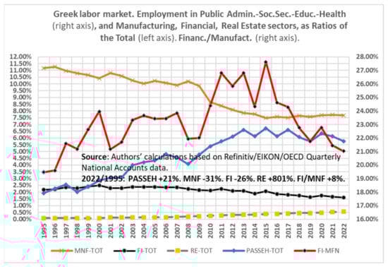
Figure A1.
Huge changes in the labor market especially since the GFC-2008. PASSEH-TOT = employment in public administration, social security, education, and health as a ratio of the total employment; MFN (FI) [RE]-TOT = manufacturing (financial and insurance activities) [real estate activities] employment as a ratio of the total; FI-MFN = financial and Insurance Activities’ employment as a ratio of the manufacturing one.

Figure A2.
Profitability of the financial sector and manufacturing, as well as current GDP (sa). GOS-S11GDP = gross operating surplus (GOS) of non-financial firms (S.11) to GDP ratio; GOS-S12GDP = gross operating surplus (GOS) of financial firms (S.12) to GDP ratio; S12/S11 = ratio of the GOS of the financial to the non-financial sector; GDPCUSA = gross domestic product, current prices, seasonally adjusted.
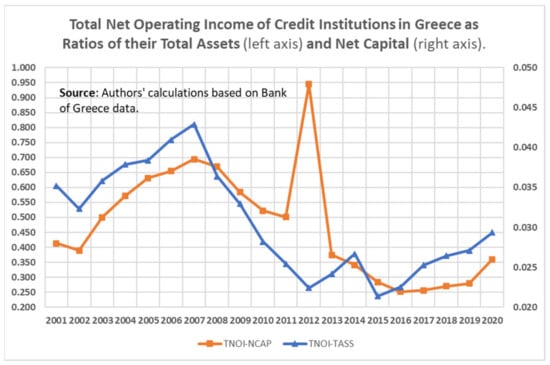
Figure A3.
Profitability of credit Institutions. TNOI-TASS = total net operating income of credit institutions in Greece (=net interest income + net fee and commission income + dividend income + net gains on financial transactions + other income) as ratio of their total assets; TNOI-NCAP = Total net operating income of credit institutions in Greece as ratios of their net capital.
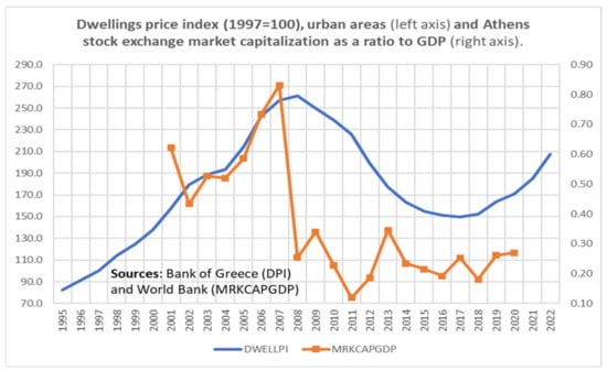
Figure A4.
Asset prices and relative values. DWELLPI = index prices of dwellings (historical series), urban areas, 1997 = 100; MRKCAPGDP = Greece, capital markets, market capitalization of listed domestic companies (% of gross domestic product).
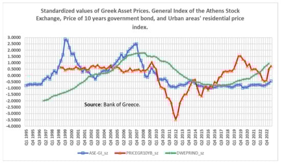
Figure A5.
Volatility of asset prices. ASE-GI_sz = standardized form of the ASE general price index based on the share price indices of the Athens Exchange (ASE); PRICEGR10YB_sz = standardized form of the price of 10-year Greek government bonds based on the financial markets, Greek government securities; DWEPRIND_sz = standardized form of the index prices of dwellings based on the residential property indices.
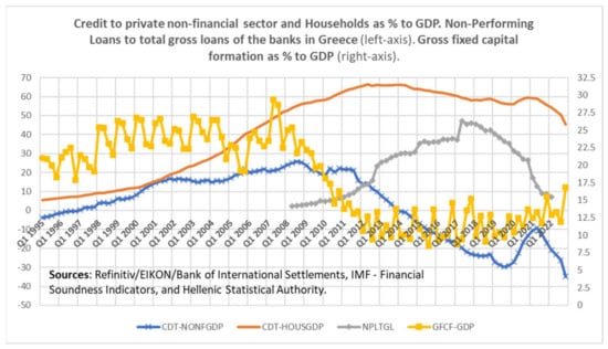
Figure A6.
Credits, NPL and private investments to GDP. CDT-NONFGDP = credit to non-financial corporations as a ratio of the GDP; CDT-HOUSGDP = credit to households as a ratio of the GDP; NPLTGL = nonperforming loans to total gross loans, financial soundness indices; GFCF-GDP = gross fixed capital formation (private fixed investments) to GDP ratio.
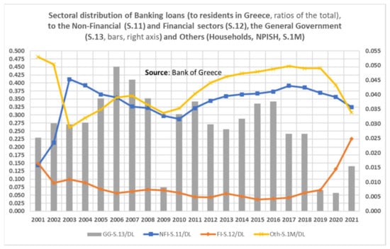
Figure A7.
Distribution of banking loans. NFI-S.11/DL = loans to non-financial corporations as a ratio of total banking loans; FI-S.12/DL = loans to financial institutions as a ratio of total banking loans; GG-S.13/DL = loans to the general government as a ratio of total banking loans; Oth-S.1M/DL = loans to households and NPISH as a ratio of total banking loans.
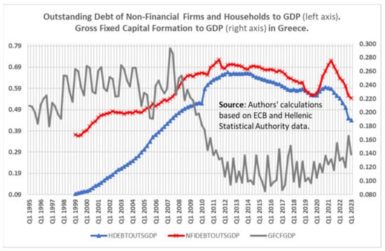
Figure A8.
Debts and investments. HDEBTOUTSGDP = households and NPISH debt outstanding to GDP; NFIDEBTOUTSGDP = nonfinancial corporations debt outstanding to GDP; GFCFGDP = gross fixed capital formation (private fixed investments) to GDP ratio.
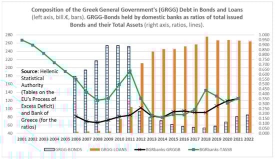
Figure A9.
Government’s bonds and loans, as well as domestic banks’ holding. BGRbank-GRGGB (TASSB) = ratio of the Greek general government bonds held by domestic banks to total issued (to their total assets); GRGG-BONDS = Greek bonds held by domestic banks; GRGG-LOANS = Greek loans of the general government’s debt (end of periods, current prices, mill. €).
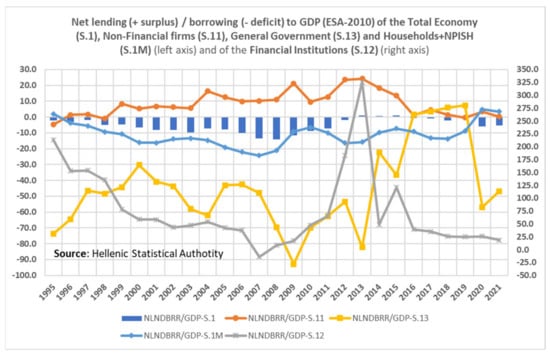
Figure A10.
Overall performance of institutional sectors. Where: NLNDBRR/GDP-S.1 = ratio of net lending (+)/net borrowing (-) (B.9) of the total economy (S.1) to GDP (B.1g); NLNDBRR/GDP-S.11(S.12) [S.13] {S.1M} = ratio of net lending (+)/net borrowing (-) (B.9) of non-financial corporations (financial institutions) [general government] {households and NPISH} to GDP (B.1g).
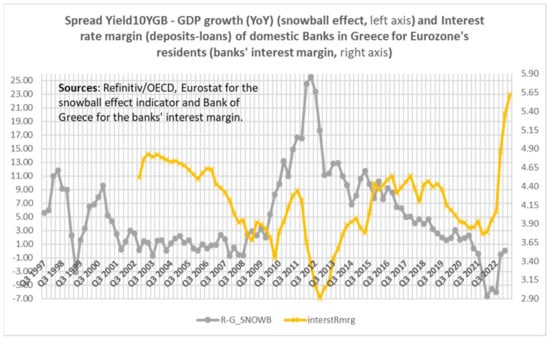
Figure A11.
Snowball effect and interest rate margin of domestic banks. R-G_SNOWB = spread between the 10 years government bond yield (r) and the growth rate of nominal GDP (g); InterstRmrg = interest rate margin (average interest rates on loans—deposits) of domestic banks.
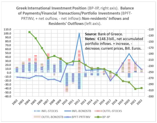
Figure A12.
Obvious domestic structural deficiencies and double financial fragility. INFL-STOCKS = Greece, portfolio investments in domestic stocks from non-residents (liabilities); INFL-BONDSTB = Greece, portfolio investments in domestic bonds and treasury bills from non-residents (liabilities); OUTFL-STOCKS = Greece, portfolio investments in foreign stocks from residents (requirements); OUTFL-BONDSTB = Greece, portfolio investments in foreign bonds and treasury bills from residents (requirements); BPFT-PRTFINV = Greece, balance of payments, balance of financial transactions, portfolio investments; BP-IIP = Greece, balance of payments, international investment position.
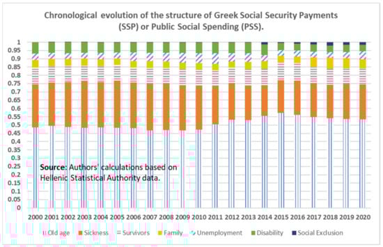
Figure A13.
The anelastic composition of the PSS.
Notes
| 1 | Strictly speaking, Greece, along with Italy, Spain, Portugal and Ireland, is considered to belong to the South-West Euro Area Periphery (SWEAP) as opposed to the core member countries of the Eurozone (Aizenman et al. 2013). |
| 2 | European System of Integrated Social Protection Statistics (ESSPROS): a nominal convergence of Greece towards EMU is reported in aggregated benefits and grouped schemes—in % of GDP; these total social transfers were, on average (stdev), 19.3% (1.4%) for Greece during 1995–2008, and for the Euro area (19 countries), 25.1% (0.4%) during 2000–2008; for Greece, 25.9% (1.0%) and for the Euro area (19 countries), 27.9% (0.3%) during 2009–2019. https://ec.europa.eu/eurostat/databrowser/view/spr_exp_gdp__custom_9184255/default/line?lang=en accessed on 17 January 2024. |
| 3 | So, FFH ≡ eFIH + EZFH. |
| 4 | Memorandum of understanding. |
| 5 | International Monetary Fund (IMF), European Commission (EC) and European Central Bank (ECB). |
| 6 | Pandemic emergency purchasing program of the European Central Bank (ECB). |
| 7 | Outright monetary transactions of the ECB. |
| 8 | Recovery and resilience fund. |
| 9 | In their sample of 21 OECD countries during the period 1982–2003, Luxembourg and Greece are the missing EU members. |
| 10 | Only the underlined categories of benefits are offered in Greece. |
| 11 | Resulting from wrong economic policies adopted by the European authorities, such as the OMT (outright monetary transactions) program announced by the ECB but under the condition of austerity rules imposed by the ESM (European Stability Mechanism). This was the case of the SWEAP countries. |
| 12 | Next-generation European Union plan. |
| 13 | Based on the Hellenic Statistical Authority’s (HAS’s) data and communications (https://www.statistics.gr/en/statistics/-/publication/SHE24/- accessed on 17 January 2024). The hierarchical presentation of these categories of benefits is based on the realized average payments in 2020, which is referred by the HSA as the last year of available annual data 2000–2020. |
| 14 | The latest available annual HSA data (Hellenic Statistical Authority) show that, on average (standard deviation), the share of pensions (age plus survivors), health and disability–incapacity in public social spending was 91% (2.1%) during the period 2000–2020; the rest was either unemployment or family benefits, with 4% (0.9%) each. |
| 15 | The balanced fiscal budget should, in the recession of the crisis period, be in surplus so as to find ways of repaying the sovereign debt. Harsh austerity–deflation policy… |
| 16 | Proxy of the “Financial development” (Choi et al. 2017). |
| 17 | |
| 18 | |
| 19 | “The first account in the sequence is the production account, which records the output and inputs of the production process, leaving value added as the balancing item. The value added is taken forward to the next account which is the generation of income account. Here the compensation of employees in the production process is recorded, as well as taxes due to government because of the production, so that the operating surplus (or mixed income from the self-employed of the households’ sector) can be derived as the balancing item for each sector.” (ESA 2010, p. 53). That is, the gross operating surplus (GOS) used here as a measure of the profitability of sectors does not include any financial expenses or receipts (interest or principal of a debt). |
| 20 | Balance of payments—international investment position. |
| 21 | The term ‘net lending/net borrowing’ is a sort of terminological shortcut. When the variable is positive (meaning that it shows a financing capacity), it should be called net lending (+); when it is negative (meaning that it shows a borrowing need), it should be called net borrowing (−). (ESA 2010, p. 466). |
| 22 | The net lending (+) or borrowing (−) of the total economy is the sum of the net lending or borrowing of the institutional sectors. It represents the net resources that the total economy makes available to the rest of the world (if it is positive) or receives from the rest of the world (if it is negative). The net lending (+) or borrowing (−) of the total economy is equal but of opposite sign to the net borrowing (−) or lending (+) of the rest of the world. (ESA 2010, p. 306). |
| 23 | It is not possible from macroeconomic data to “prove” whether a firm’s or household’s loan is being repaid “regularly” (hedge financing structure), or in a Eurozone country, or if only interest is being paid by firms (hyper-speculative) or not serviced at all (Ponzi). However, when the outstanding debts of the non-financial sector increase, while at the same time, it is excluded from bank credit, NPLs proliferate or, finally, the government defaults or the international investment position of the country continuously deteriorates, the evidence is sufficiently strong to characterize the sub-periods of the sample according to the Minsky classification. |
| 24 | Non-profit institution serving households (see, ESA 2010). |
| 25 | Money supply measure. |
| 26 | r = weighted average of the interest rate of the government’s outstanding debt; g = real gross domestic product (GDP) growth rate. |
| 27 | STATA/SE version 17 software has been used, provided by the University of West Attica academic license. |
| 28 | When we alternatively used the variable “nprtfinflowsgdp” (also drawn from the Bank of Greece dataset and balance of financial account), the estimated coefficient also statistically significant at 5% level this time had a negative sign, −0.058. |
| 29 | We emphasize that this is performed in a long-term equilibrium, or the series are cointegrated. |
| 30 | Which (old age + sickness + survivors) aggregate to an average of almost 85% of the total PSS (see, Figure A13 in Appendix A). |
| 31 | That have taken into account in the determinants of Equation (3). |
| 32 | This characterizes almost permanently the lack of international competitiveness and the respective trade balance deficit of the country. |
| 33 | Mergers and acquisitions. |
| 34 | The majority of more than 80% of the Greek production sector. |
| 35 | It should be stressed that the austerity–deflationary policies that were implemented (which reduced real Greek GDP by 25% and increased unemployment to 27% in the period 2008–2015) not only reduced aggregate demand but also aggregate supply due to the restructuring of sectors and markets brought about by the successive crises. |
| 36 | Credit rating agencies. |
| 37 | It is a matter of special paper(s) to reconsider democratic decision making (including economic policy) in Europe... Greece marked human history and civilization, both with “polis («πόλις»)-democracy” and with “critical thinking” who lived in ancient Greek «πόλεις» or Eastern Romanian Empire or even under Ottoman Empire and occupation, at least until 1832. So, it worked historically. Few words can be reported: the first one, (πόλις) democracy, means another way of collectiveness institutionally and functionally homologous to “truth” (i.e., that which does not wear out does not die), while the criterion in the second (critical thought), i.e., how can one distinguish right–wrong, truth–false, valid knowledge–illusion, is the “common experience” of all citizens, and not principles of utilitarian efficiency that we economists use, insisting only on the “society of needs” and not, as people worldwide demand, also the “society of human relations”. (Yannaras 2011). |
References
- Aizenman, Joshua, Michael Hutchison, and Yothin Jinjarak. 2013. What is the Risk of European Sovereign Debt Defaults? Fiscal Space, CDS Spread and Market Pricing of Risk. Journal of International Money and Finance 34: 37–59. [Google Scholar] [CrossRef]
- Alary, Pierre, and Elsa Lafaye de Micheaux. 2015. Capitalismes Asiatiques et Puissance Chinoise: Diversité et Recomposition des Trajectoires Nationales, 1st ed. Paris: Sciences Po. Les Presses. ISBN 2724616200. [Google Scholar]
- Amoutzias, Chrysovalantis. 2019. An investigation of the effects of income inequality on financial fragility: Evidence from Organization for Economic Co-operation and Development countries. International Journal of Finance & Economics 24: 241–59. [Google Scholar]
- Arestis, Philip, and Murray Glickman. 2002. Financial crisis in Southeast Asia: Dispelling illusion the Minskyan way. Cambridge Journal of Economics 26: 237–60. [Google Scholar] [CrossRef]
- Besedovsky, Natalia. 2018. Financialization as calculative practice: The rise of structured finance and the cultural and calculative transformation of credit rating agencies. Socio-Economic Review 16: 61–84. [Google Scholar] [CrossRef]
- Blanchard, Olivier, Alessia Amighini, and Francesco Giavazzi. 2021. Macroeconomics: A European Perspective, 4th ed. London: Pearson. Available online: https://www.pearson.com/en-gb/subject-catalog/p/macroeconomics-a-european-perspective/P200000003747?view=educator (accessed on 12 December 2023).
- Boyer, Robert. 2000. Is a Finance-led Growth Regime a Viable Alternative to Fordism? A Preliminary Analysis. Economy and Society 29: 111–45. [Google Scholar] [CrossRef]
- Boyer, Robert. 2013. Origins and ways out of the euro crisis: Supranational institution building in the era of global finance. Contributions to Political Economy 32: 97–126. [Google Scholar] [CrossRef]
- Boyer, Robert. 2022. The Transformations of Contemporary Capitalisms: Seven Lessons. In Rethinking Asian Capitalism: The Achievements and Challenges of Vietnam Under Doi Moi. Edited by Thi Anh-Dao Tran. London: Palgrave Macmillan, pp. 25–58. [Google Scholar]
- Boyer, Robert, and Yves Saillard, eds. 2002. Régulation Theory: The State of the Art. London: Routledge. [Google Scholar]
- Boyer, Robert, Hiroyasu Uemura, and Akinori Isogai, eds. 2011. Diversity and Transformations of Asian Capitalisms. London: Routledge. [Google Scholar] [CrossRef]
- Choi, Sangyup, Davide Furceri, and João Tovar Jalles. 2017. Fiscal Stabilization and Growth: Evidence from Industry-Level Data for Advanced and Developing Economies. IMF Working Paper No. 2017/198. Washington: International Monetary Fund. [Google Scholar]
- Christophers, Brett, and Ben Fine. 2020. The value of financialization and the financialization of value. In The Routledge International Handbook of Financialization. Edited by Philip Mader, Daniel Mertens and Natascha van der Zwan. New York: Taylor & Francis, pp. 19–30. Available online: https://bookshelf.vitalsource.com/books/9781351390361 (accessed on 15 June 2023).
- Cibils, Alan, and Cecilia Allami. 2013. Financialisation vs. Development Finance: The Case of the Post-Crisis Argentine Banking System. Revue de la Régulation 13. [Google Scholar] [CrossRef]
- Darby, Julia, and Jacques Melitz. 2008. Social spending and automatic stabilizers in the OECD. Economic Policy 23: 715–56. [Google Scholar] [CrossRef]
- De Grauwe, Paul. 2011. The European Central Bank: Lender of Last Resort in the Government Bond Markets? Working Paper No. 3569. Munich: Center for Economic Studies, Ludwig-Maximilians-Universität, and Ifo Institute (CESifo). Available online: https://www.cesifo.org/en/publications/2011/working-paper/european-central-bank-lender-last-resort-government-bond-markets (accessed on 15 June 2023).
- De Grauwe, Paul. 2012. The governance of a fragile Eurozone. The Australian Economic Review 45: 255–68. [Google Scholar] [CrossRef]
- De Grauwe, Paul. 2013. Design Failures in the Eurozone: Can They Be Fixed? LSE Europe in Question Discussion Paper Series No. 57; Available online: https://ec.europa.eu/economy_finance/publications/economic_paper/2013/ecp491_en.htm (accessed on 15 June 2023).
- De Grauwe, Paul, and Yuemei Ji. 2022. The fragility of the Eurozone: Has it disappeared? Journal of International Money and Finance 120: 102546. [Google Scholar] [CrossRef]
- Dow, Sheila. 2020. Financialization, money and the state. In The Routledge International Handbook of Financialization. Edited by Philip Mader, Daniel Mertens and Natascha van der Zwan. New York: Taylor & Francis, pp. 56–67. Available online: https://bookshelf.vitalsource.com/books/9781351390361 (accessed on 15 June 2023).
- Epstein, Gerald A. 2005. Financialization and the World Economy. Northampton: Edward Elgar. ISBN 978 1 84376 874 6. [Google Scholar]
- European System of Accounts. 2010. Available online: https://ec.europa.eu/eurostat/web/products-manuals-and-guidelines/-/ks-02-13-269 (accessed on 8 May 2024).
- Fatás, Antonio, and Ilian Mihov. 2003. The case for restricting fiscal policy discretion. The Quarterly Journal of Economics 118: 1419–47. [Google Scholar] [CrossRef]
- Goel, Rajeev K., James E. Payne, and Rati Ram. 2008. R&D expenditures and U.S. economic growth: A disaggregated approach. Journal of Policy Modeling 30: 237–50. [Google Scholar] [CrossRef]
- Hajilee, Massomeh, Donna Y. Stringer, and Linda A. Hayes. 2021. On the link between the shadow economy and stock market progress: An asymmetry analysis. The Quarterly Review of Economics and Finance 80: 303–16. [Google Scholar] [CrossRef]
- Hepburn, Brian, and Hanne Andersen. 2021. Scientific Method. In The Stanford Encyclopedia of Philosophy, Summer 2021 ed. Edited by Edward N. Zalta. Available online: https://plato.stanford.edu/archives/sum2021/entries/scientific-method/ (accessed on 1 May 2024).
- Holloway, Matthew, and Jari Eloranta. 2014. “Stability breeds instability?” A Minskian analysis of the Asian crisis of the Tigers in the 1990s. Investigaciones de Historia Económica—Economic History Research 10: 115–26. [Google Scholar] [CrossRef]
- Krippner, Greta R. 2005. The financialization of the American economy. Socio-Economic Review 3: 173–208. [Google Scholar] [CrossRef]
- Kuhn, Thomas S. 1962. The Structure of Scientific Revolutions. Chicago: University of Chicago Press. [Google Scholar]
- Kyriakopoulos, Dionysios, John Yfantopoulos, and Theodoros V. Stamatopoulos. 2022. Social Security Payments and Financialization: Lessons from the Greek Case. Journal of Risk and Financial Management 5: 615. [Google Scholar] [CrossRef]
- Lapavitsas, Costas. 2009. Financialised Capitalism: Crisis and Financial Expropriation. Historical Materialism 17: 114–48. [Google Scholar] [CrossRef]
- Mader, Philip, Daniel Mertens, and Natascha van der Zwan. 2020. The Routledge International Handbook of Financialization. New York: Taylor & Francis. Available online: https://bookshelf.vitalsource.com/books/9781351390361 (accessed on 15 June 2023).
- Minsky, Hyman P. 1957. Central banking and money market changes. Quarterly Journal of Economics 71: 171–87. [Google Scholar] [CrossRef]
- Minsky, Hyman P. 1975. John Maynard Keynes. New York: Columbia University Press. [Google Scholar]
- Minsky, Hyman P. 1977. A theory of systemic fragility. In Financial Crises: Institutions and Markets in a Fragile Environment. Edited by Edward I. Altman and Arnold W. Sametz. New York:: John Wiley & Sons, pp. 138–52. Available online: https://digitalcommons.bard.edu/hm_archive/231/ (accessed on 10 May 2023).
- Minsky, Hyman P. 1978. The Financial Instability Hypothesis: A Restatement. Annandale-on-Hudson: Levy Economics Institute of Bard College. Available online: https://digitalcommons.bard.edu/hm_archive/180/ (accessed on 10 May 2023).
- Minsky, Hyman P. 1982. Can “It” Happen Again? Essays in Instability and Finance. Reprint by Routledge 11 April 2016. Armonk: M. E. Sharpe. ISBN 9781138641952. Available online: https://www.routledge.com/Can-It-Happen-Again-Essays-on-Instability-and-Finance/Minsky/p/book/9781138641952 (accessed on 10 May 2023).
- Minsky, Hyman P. 1983. The financial instability hypothesis: An interpretation of Keynes and an alternative to “standard” theory. In John Maynard Keynes: Critical Assessments. Edited by John Cunningham Wood. London: Macmillan, pp. 282–92. [Google Scholar]
- Minsky, Hyman P. 1986. Stabilizing an Unstable Economy. Annandale-on-Hudson: Levy Economics Institute of Bard College. Available online: https://digitalcommons.bard.edu/hm_archive/144/ (accessed on 10 May 2023).
- Minsky, Hyman P. 1992a. The Financial Instability Hypothesis. Working Paper No. 74. Annandale-on-Hudson: Levy Economics Institute of Bard College. [Google Scholar]
- Minsky, Hyman P. 1992b. Hyman P. Minsky. In A Bibliographical Dictionary of Dissenting Economists. Edited by Philip Arestis and Malcolm C. Sawer. Aldershot: Edward Elgar. Available online: https://www.e-elgar.com/shop/gbp/a-biographical-dictionary-of-dissenting-economists-second-edition-9781858985602.html (accessed on 10 May 2023).
- Minsky, Hyman P. 1995. Financial factors in the economics of capitalism. Journal of Financial Services Research 9: 197–208. [Google Scholar] [CrossRef]
- Minsky, Hyman P. 1996. Uncertainty and the Institutional Structure of Capitalist Economies. Journal of Economic Issues 30: 357–68. [Google Scholar] [CrossRef]
- Palley, Thomas I. 2007. Financialisation: What It Is and Why It Matters. Working Paper No. 525. Annandale-on-Hudson: The Levy Economics Institute of Bard College. [Google Scholar]
- Pesaran, M. Hashem, and Yongcheol Shin. 1999. An Autoregressive Distributed Lag Modelling Approach to Cointegration Analysis. In Econometrics and Economic Theory in the 20th Century: The Ragnar Frisch Centennial Symposium. Edited by Steinar Strøm. Cambridge: Cambridge University Press, pp. 371–413. [Google Scholar] [CrossRef]
- Pesaran, M. Hashem, Yongcheol Shin, and Richard J. Smith. 2001. Bounds testing approaches to the analysis of level relationships. Journal of Applied Economics 16: 289–326. [Google Scholar] [CrossRef]
- Pierros, Christos. 2020. Income distribution, structural competitiveness and financial fragility of the Greek economy. International Review of Applied Economics 34: 50–74. [Google Scholar] [CrossRef]
- Popper, Karl. 2002. The Logic of Scientific Discovery. New York: Routledge. ISBN 9780415278447. [Google Scholar]
- Rossi, Sergio. 2013. Financialisation and monetary union in Europe: The monetary–structural causes of the euro-area crisis. Cambridge Journal of Regions, Economy and Society 6: 381–400. [Google Scholar] [CrossRef]
- Sen, Sunanda. 2020. Financialization, speculation and instability. In The Routledge International Handbook of Financialization. Edited by Philip Mader, Daniel Mertens and Natascha van der Zwan. New York: Taylor & Francis, pp. 448–57. Available online: https://bookshelf.vitalsource.com/books/9781351390361 (accessed on 15 June 2023).
- Sotiropoulos, Dimitris P., and Ariane Hillig. 2020. Financialization in heterodox economics. In The Routledge International Handbook of Financialization. Edited by Philip Mader, Daniel Mertens and Natascha van der Zwan. New York: Taylor & Francis, pp. 125–35. Available online: https://bookshelf.vitalsource.com/books/9781351390361 (accessed on 15 June 2023).
- van der Zwan, Natascha. 2014. Making sense of financialization. Socio-Economic Review 1: 99–129. [Google Scholar] [CrossRef]
- Vigny, Léo. 2022. The Greek Sovereign Crisis: A Post-Keynesian Synthesis. International Journal of Political Economy 51: 151–69. [Google Scholar] [CrossRef]
- Wade, Robert. 1990. Governing the Market: Economic Theory and the Role of Government in East Asian Industrialization. Princeton: Princeton University Press. [Google Scholar] [CrossRef]
- Yannaras, Cristos. 2011. Six Philosophical Paintings. Athens: IKAROS Publishers. ISBN 13 9789609527248. [Google Scholar]
Disclaimer/Publisher’s Note: The statements, opinions and data contained in all publications are solely those of the individual author(s) and contributor(s) and not of MDPI and/or the editor(s). MDPI and/or the editor(s) disclaim responsibility for any injury to people or property resulting from any ideas, methods, instructions or products referred to in the content. |
© 2024 by the authors. Licensee MDPI, Basel, Switzerland. This article is an open access article distributed under the terms and conditions of the Creative Commons Attribution (CC BY) license (https://creativecommons.org/licenses/by/4.0/).