Abstract
The currency exchange rate is a crucial link between all countries related to economic and trade activities. With increasing volatility, exchange rate fluctuations have become frequent under the combined effects of global economic uncertainty and political risks. Consequently, accurate exchange rate prediction is significant in managing financial risks and economic instability. In recent years, the Transformer models have attracted attention in the field of time series analysis. Transformer models, such as Informer and TFT (Temporal Fusion Transformer), have also been extensively studied. In this paper, we evaluate the performance of the Transformer, Informer, and TFT models based on four exchange rate datasets: NZD/USD, NZD/CNY, NZD/GBP, and NZD/AUD. The results indicate that the TFT model has achieved the highest accuracy in exchange rate prediction, with an R2 value of up to 0.94 and the lowest RMSE and MAE errors. However, the Informer model offers faster training and convergence speeds than the TFT and Transformer, making it more efficient. Furthermore, our experiments on the TFT model demonstrate that integrating the VIX index can enhance the accuracy of exchange rate predictions.
1. Introduction
The exchange rate is a fundamental economic factor, significantly impacting domestic and international economic relations. The exchange rate acts as a bridge for financial communication between various countries (Pradeepkumar and Ravi 2018). Its instabilities not only affect the country’s international trade and capital flows but also directly impact the international investment of enterprises, foreign trade and individual investment. Forecasting exchange rate trends is an essential basis for judging the timing of exchange rate transactions.
The exchange rate market is a nonlinear dynamic market characterized by complexity, diversity and uncertainty (Niu and Zhang 2017). This makes exchange rate forecasting more challenging. With the advent of artificial intelligence, the existing research work on financial time series forecasting has also obtained more and more attention. In contrast to traditional time series methods, it can manage the nonlinear, chaotic, noisy and complex data of exchange rate markets, allowing for more effective forecasts (Rout et al. 2017). The dataset is crucial in exchange rate forecasting, mainly including exchange rate prices, volatility, etc. However, if the selected time series is long and has high dimensions, it is tough to achieve the expected results by using the existing models for exchange rate prediction (Lai et al. 2018). Afterward, with the rapid growth in artificial intelligence (AI), the usage of deep learning models to process time-series-related tasks has recently become mainstream, and a series of neural network models for time series tasks has appeared. Early proposed models such as Recurrent Neural Networks (RNN), Long Short-Term Memory (LSTM) and Gated Recurrent Unit (GRU) are considered suitable for processing time series tasks (Pirani et al. 2022).
As the most popular mainstream architecture of deep learning in recent years, the Transformer models are widely adopted in typical tasks such as text classification, sentiment analysis, target detection, speech recognition, etc. However, there are few related works in the field of time series analysis, and multiple financial time series analysis research works still use traditional sequence prediction methods. Therefore, this paper proposes the research questions as follows:
- Question 1: How does the Transformer model perform in predicting the exchange rate?
- Question 2: By comparing the Transformer, Informer and Temporal Fusion Transformer, which algorithm performs best in predicting the exchange rate?
This paper aims to achieve exchange rate predictions based on NZD and discover the most advanced algorithms fitting for exchange rate predictions through deep learning. Based on transformers, we have studied two recent algorithms, Informer and TFT. During our experiments on Google Colab, we trained the model, adjusted parameters, and obtained results established on four processed datasets. Subsequently, the performance of the three algorithms was compared and analyzed to determine the optimal forecast exchange rate model. Eventually, this paper explored the pros and cons of the model, summarized the experimental results, and provided references for other related research work.
The structure of this paper is outlined as follows: Section 2 presents the related works and elaborates on the methodologies of the three models. Section 3 displays the results through experiments on the three models. Section 4 contains the conclusion by comparing the performance of the three models and analyzing them in conjunction with their own characteristics.
2. Materials and Methods
This section consists of related work based on traditional time series models and proposed models: Transformer, Informer, and TFT. In addition, it also illustrates the corresponding methodologies. Subsequently, the experimental processes are presented, and the measures for model evaluation are clarified.
2.1. Related Work Based on Traditional Time Series Models
Since the exchange rate is non-stationary in mean and variance, its relationship with other data series changes dynamically due to nonlinear and dynamic changes in the exchange rate over time (Xu et al. 2019). As international trade continues to grow at an increasing rate, it is becoming more and more common, and the factors affecting exchange rates gradually increase.
2.1.1. ARIMA
ARIMA is one of the most universal linear methods for forecasting time series, and its research has achieved great success in academic and industrial applications (Khashei and Bijari 2011). In the study of the USD/TRY exchange rate forecast, Yıldıran and Fettahoğlu (2017) generated long-term and short-term models based on the ARIMA framework. Through comparison, it was found that ARIMA is more fitting for short-term forecasts. Similarly, Yamak et al. (2019) used a dataset of Bitcoin prices and applied the ARIMA, LSTM and GRU models for prediction analysis. The results showed that ARIMA delivered the best results among these models, with a MAPE and RMSE of 2.76% and 302.53, respectively.
2.1.2. RNN
RNN is one of the neural networks specifically designed to handle time series problems (Hu et al. 2021). It can extract information from a time series, allow the information to persist, and use previous knowledge to infer subsequent patterns. Traditional neural networks such as the Backpropagation Neural Network (BPNN) are also used for time series modeling, while the time series information of such models is usually less than RNN.
2.1.3. LSTM
Although RNN has outstanding advantages in dealing with time series problems, as the training time rises and the number of network layers increases after the nodes of the neural network have been calculated in many stages, the features of the previous relatively long time slice have been covered, so problems such as vanishing gradient or exploding gradient are prone to occur, which leads to the incapability to learn the relationship between information, thereby losing the ability to process long-term series data (Li et al. 2018).
2.2. Related Work Based on Transformer, Informer, and TFT
2.2.1. Transformer
Transformer was initially explored by Vaswani et al. (2017), and it no longer stuck to the framework of RNN and CNN, and attention was applied to the seq-to-seq structure to form the Transformer model and to process natural language tasks. Since then, the Transformer model has generated outstanding results in fields such as computer vision (Han et al. 2022). Moreover, the research work on Transformer in time series has also aroused great interest (Wen et al. 2023). Through experimental research on 12 public datasets with time series, it was found that Transformer can capture long-term dependencies and obtain the most accurate prediction results in five of the dataset trainings (Lara-Benítez et al. 2021). However, its calculation is more complex than CNN, so the training process is relatively slow.
Despite in-depth research outcomes on the Transformer, it is evident from the literature that most studies primarily focus on reducing the computational requirements of the Transformer model (Tay et al. 2022). However, they overlook the importance of capturing the dependencies among neighboring elements, addressing the heterogeneity between the values of time series data, the temporal information corresponding to the time series, and the positional information of each dimension within the time series.
2.2.2. Informer
To solve the heterogeneity of time information, position information and numbers, a model based on Transformer architecture and attention mechanism was offered (Zhou et al. 2021). For the first time, time coding, position coding and scalar were introduced in the embedding layer to crack the long sequence input problem. ProbSparse self-attention captures long-distance dependencies and lessens the time complexity in the computation process. Using the distillation mechanism can effectively decrease the time dimension of the feature map and lower memory consumption. Although Informer outperforms LSTM in time series forecasting tasks, its inability to capture dependencies among neighboring elements with a multihead attention mechanism leads to insufficient capture of the time series local information. This results in lower prediction accuracy and higher memory consumption, which could be more conducive to large-scale deployment. A relative coding algorithm (Gong et al. 2022) was based on the Informer framework to predict the heating load. The experimental results indicate that the improved Informer model is more robust. Moreover, based on Informer and the proposed Autoformer (Wu et al. 2021), a new decomposition architecture was designed with an autocorrelation mechanism. The model breaks the preprocessing convention of sequence decomposition and updates it into the fundamental internal blocks of the deep model. This design enables Autoformer to progressively decompose complex time series. Moreover, inspired by the random process theory, Autoformer designed an autocorrelation mechanism based on sequence periodicity, replacing the Self-Attention module in Transformer with autocorrelation mode. In long-term forecasting, Autoformer achieves outstanding accuracy.
2.2.3. TFT
Transformer model has demonstrated its outstanding performance in both natural language processing and computer vision (Bi et al. 2021). Applying this model to capture long-term dependencies and data interaction in time series has become the focus. The general method for processing time series data is to treat data in all dimensions with equal weight. This may cause the model to ignore critical input information or be interfered with by noise, which is also a shortcoming of traditional processing methods. Temporal Fusion Transformer (TFT) is a Transformer model for multistep prediction tasks, which is developed to effectively process different types of input information (i.e., static, known or observed inputs) and construct feature representations to achieve high predictive performance (Lim et al. 2021). The TFT model (Zhang et al. 2022) was proposed to predict short-term highway speed by collecting Minnesota traffic data and applying them to the training and testing of the model. Compared with traditional models, the TFT model performs best when the prediction range exceeds 30 min.
2.3. Methods Based on Transformer, Informer and TFT
2.3.1. Transformer
In Transformers, the self-attention mechanism has received a higher recognition rate compared to other neural network models that utilize the attention mechanism. The attention mechanism in Transformers excels at capturing the internal correlation within data and features, and more effectively solves the problem of long-distance dependence (Wang et al. 2022).
Contrary to other models that only make use of a single attention module, the Transformer employs multihead attention modules to operate in parallel (Sridhar and Sanagavarapu 2021). In this step, the original queries, keys and values of dimension are each mapped into spaces of dimensions , and using H different learned vectors. The model computes each of these mapped queries, keys and values according to Equation (1), outputting attention weights for each. Then, it concatenates all these outputs and converts them back into an dimensional representation.
where is computed by applying the attention function to the transformed inputs. represents the weight matrix applied after concatenating the outputs of all attention heads.
2.3.2. Informer
Informer model has been proposed to address the long-sequence forecasting issues in the Transformer. This model provides an improved self-attention module to reduce time complexity (Sun et al. 2022).
In the Informer network, probabilistic sparse self-attention replaces traditional self-attention. Each input vector is utilized to calculate query, key and value vectors in the self-attention mechanism. Then, attention weights are calculated by computing the dot product of query vectors and key vectors. The attention weights represent the similarity between each and all input vectors. In the probabilistic sparse self-attention mechanism, query vectors compute the similarity with each key vector, generating an attention distribution. The probabilistic sparse self-attention calculation is shown in Equation (2).
where represents the distance calculated using KL divergence among the attention distribution and the uniform distribution to determine the value of each query point, thus specifying which queries should be allocated computational resources, it then selects the active query with the most significant distance.
In general, in probabilistic sparse self-attention calculation, attention is only given to the far-active queries. In contrast, the dot products for other queries are substituted with the mean of the value vectors, thus reducing the computational task.
2.3.3. TFT
Temporal Fusion Transformer (TFT) is a time series prediction model based on the Transformer architecture, aiming to solve the limitations of traditional time series prediction models (Lim et al. 2021). TFT introduces a novel method to capture features and nonlinear relationships across multiple time scales (Fayer et al. 2023). TFT employs recurrent layers for localized processing and interpretable attention layers to manage long-term dependencies. The algorithm also leverages specialized components for feature selection and a sequence of gating layers to filter out unnecessary elements, thereby maintaining the optimal performance of this model across various scenarios. The main components of this TFT model are the Gating mechanism and variable selection network, Static covariate encoder, and Temporal fusion decoder.
2.4. Data Collection and Preprocessing
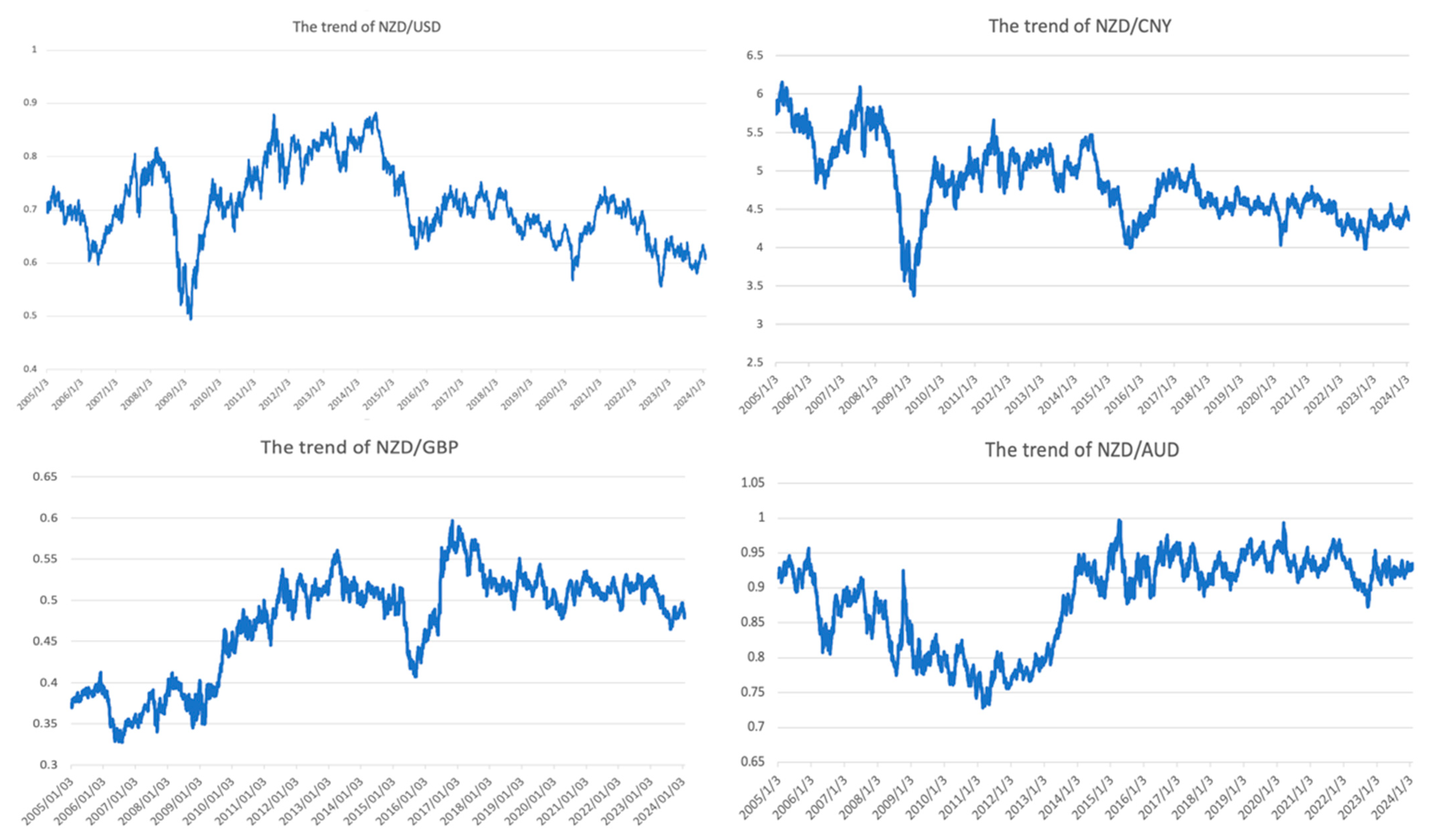
Due to the changes in the exchange rate being impacted by multiple aspects, they display diverse characteristics of change. We selected four representative currencies, USD, GBP, CNY, and AUD, as training and test samples because of their significant impact on the global economy, widespread usage in international trade, and substantial influence on foreign exchange markets. These currencies are representative of major economic regions, providing a comprehensive and diverse dataset for robust predictive modeling. The datasets of NZD against these four currencies are all from Yahoo! Finance (https://nz.finance.yahoo.com) and Investing website (www.investing.com). To enhance the learning ability of our proposed model for unexpected fluctuations, each sample includes daily data from 3 January 2005 to 2 February 2024, totaling 4980 entries. The primary variables of the dataset include closing, opening, highest, lowest and floating prices of the day. We select the closing price as the experimental objective as shown in Figure 1.
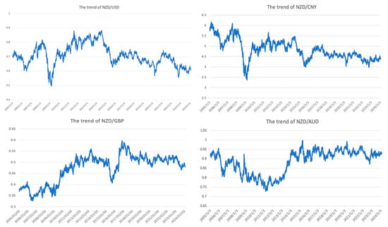
Figure 1.
The trend of NZD against the four selected currencies.
We adopt Equation (4) for imputing missing values.
where defines the data to be imputed, represents the data from the day before the missing data, and illustrates the data from the day after the missing data.
The most common method, min–max standardization, is also utilized in data preprocessing. The calculation process is
where represents the dimensionless data after normalization, X means the observation value, denotes the minimum value, and tells the maximum value. Denormalization is restoring normalized data to facilitate subsequent data analysis and other operations.
2.5. Data Description
After preprocessing the four datasets, the total number of samples for each is 4980. To better understand the data’s characteristics and distribution features and utilize the relevant data for modeling, it is essential to conduct a descriptive statistical analysis before modeling. Table 1 provides the descriptive statistics for the four datasets.

Table 1.
The descriptive statistics of NZD against four currency exchange rates.
Table 1 shows that the standard deviation for NZD/USD is 0.073, indicating that the exchange rate fluctuates within a narrow range. A kurtosis value of −0.369 and a skewness value of 0.118 suggest that the distribution of NZD/USD deviates slightly from a normal distribution, showing slight flatness and right skewness. Still, overall, it is close to symmetry. Compared to NZD/CNY, there is a significant difference between its minimum and maximum values, which are 3.371 and 6.163, respectively. The median of 4.79 is slightly lower than the average, implying a skewed distribution to the right. The standard deviation is 0.484, indicating the volatility is higher than the other three currency pairs. The kurtosis and skewness are −0.148 and 0.258, respectively, indicating a relatively flat and slightly right-skewed distribution. The statistical results for NZD/GBP show that the average exchange rate for NZD/GBP is 0.473, with a minimum of 0.328 and a maximum of 0.597, revealing a smaller fluctuation range and, hence, a relatively stable exchange rate. The median of 0.497 is very close to the mean, reflecting the central tendency of the data. Its standard deviation of 0.063 is the smallest among the four currency pairs, showing the lowest volatility. The average exchange rate for NZD/AUD is 0.884, with a fluctuation range from 0.728 to 0.997, which is relatively moderate. The median of 0.91 is higher than the average, exhibiting more data points in the higher value range. A standard deviation of 0.064 indicates lower volatility. The kurtosis of −0.886 and skewness of −0.686 present a skewed and peaked distribution, suggesting a frequent occurrence of lower values.
Throughout this detailed analysis, we summarize that these four datasets demonstrate diverse levels of volatility and distribution characteristics. NZD/GBP and NZD/AUD show relatively lower volatility, while NZD/USD and NZD/CNY exhibit higher volatility. In the experiment, we divided the dataset into two parts for the training process of the three models: 80% for training and 20% for testing.
2.6. Experiment Implementation
2.6.1. The Experimental Implementation of Transformer
In the training process of the Transformer model, it is vital to set essential parameters, which are continuously adjusted and optimized. Due to the complexity of the Transformer, we employ a lower learning rate parameter of 0.0005. Although this means that the model learns more slowly, it can help the model adapt more finely to the training data, leading to better stable and accurate predictions. The value of input_window is set to 7, which allows for more suitable capturing of weekly patterns or trends in the data for time series data like exchange rates, a typical setting in financial sequences. We experimented with the multiple training epochs, setting them at 50, 100, 150 and 200, and finally found that 150 is the best, avoiding the risk of overfitting.
2.6.2. The Experimental Implementation of Informer
Unlike the parameter settings of the Transformer, through multiple attempts, we have set the number of epochs to 60. Since the Informer optimizes computational complexity, reducing unnecessary computations and parameter usage, it achieves better results in a shorter training time. The table below details the model parameters of the Informer.
2.6.3. The Experimental Implementation of TFT
The model training of TFT is conducted within a PyTorch-lightning framework. In this environment, it is possible to adjust the model’s hyperparameters promptly during the data training process. This setup integrates with the Early-Stopping mechanism to obtain an outstanding combination of parameters. For the TFT model, a learning rate of 0.001 is a moderate value that supports balanced training speed and convergence quality. Setting the hidden layer’s size to 32 means the TFT model is relatively simple and computationally efficient. Since no overly complex recognition tasks exist, we set the number of attention heads to 1.
2.7. Evaluation Methods
In our experiment of exchange rate prediction, to reflect the reliability of the predictive performance accurately and objectively, we utilize four evaluation metrics, including root mean square error (RMSE), mean absolute error (MAE), coefficient of determination (), mean absolute percentage error (MAPE). The smaller the RMSE and MAE, the closer the predictions are to the actual values. A larger indicates a better fit of the model. MAPE provides a comprehensive indication of the model’s overall predictive effectiveness.
3. Results
3.1. Experimental Results of Transformer
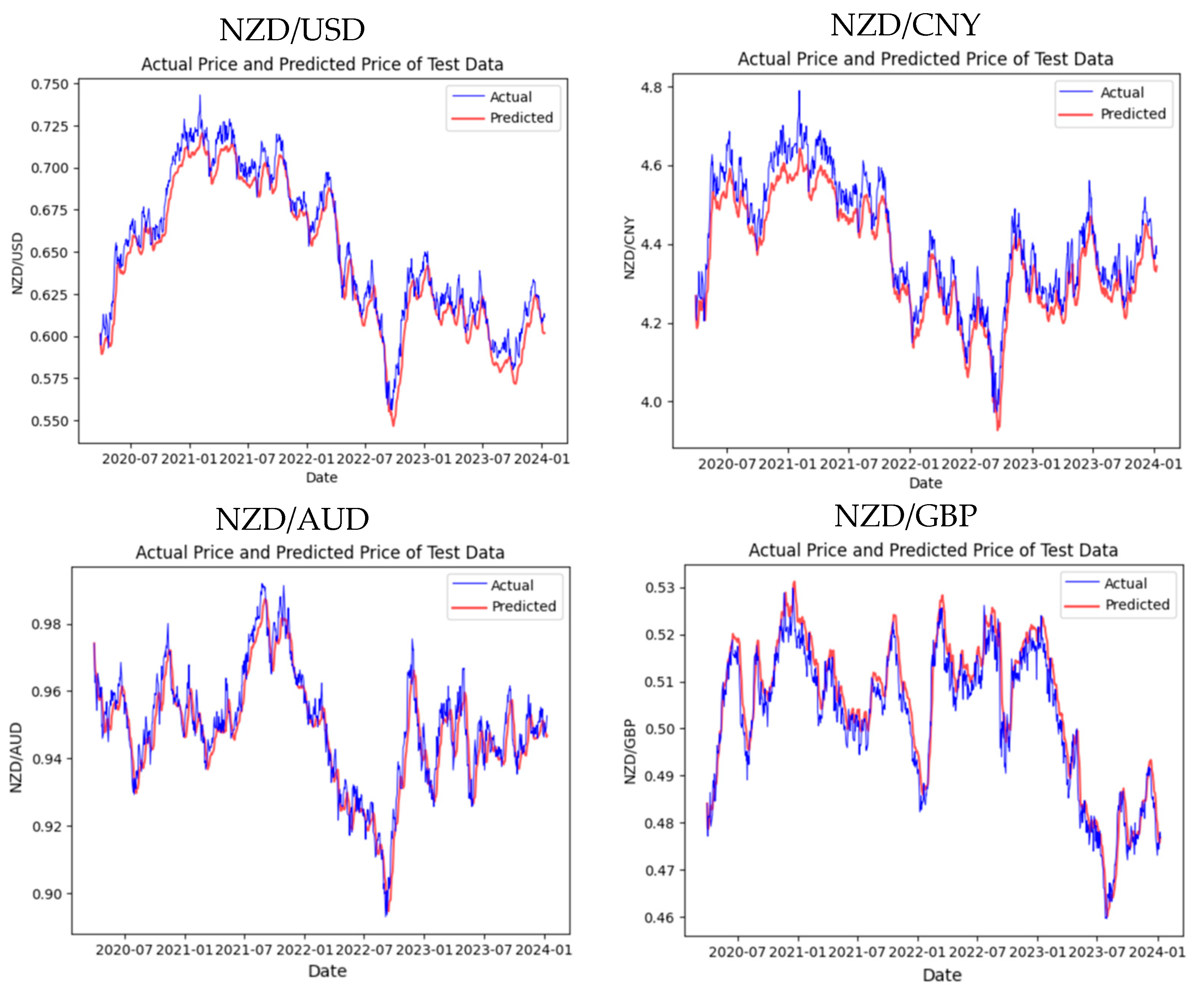
In this experiment, the initial model we trained on Google Colab for the four exchange rate datasets was the Transformer model. By considering both the training on the training set and the predictions on the test set, the Transformer has achieved satisfactory results. Figure 2 displays the actual and predictive results of the test set.

Figure 2.
The predictive results of each dataset by using Transformer.
From the prediction results related to the four test sets, the trend of NZD/USD is very close to the actual result, reaching highs and lows at almost the same time, and the high degree of overlap between the two lines indicates that the Transformer can effectively capture the trends and seasonal changes in the exchange rate. However, from the NZD/CNY prediction graph, we discover the deviations during periods of high volatility, and the Transformer model has yet to capture the peaks and troughs of the exchange rate perfectly. Despite this, the overall prediction trend still tracks the real exchange rate well. Similar to NZD/AUD, though the figure shows a strong correlation between prediction and reality, the Transformer still underestimates or overestimates the peaks in some intervals. Regarding the NZD/GBP trend, the prediction accuracy is high for most of the timeline, showing that the Transformer is robust. Table 1 shows more details of the experimental evaluation results of the Transformer.
By evaluating the model with four different indicators, we notice that in the training and prediction of the Transformer model based on the four datasets, NZD/USD exhibits remarkably high precision and reliability. The very low RMSE and MAE values show that the forecast values are extraordinarily close to the actual values. Furthermore, the low MAPE value 0.0141 verifies that the error percentage is minor, representing an ideal outcome in currency prediction. In comparison, an R2 value close to 0.94 indicates that the model has strong predictive power and a high degree of explanatory capability regarding the fluctuating exchange rate trends.
Although the MAPE values are relatively low in the NZD/CNY and NZD/AUD predictions, at 0.0113 and 0.0048, respectively, the increased RMSE and MAE indicate that the model faces more significant challenges in forecasting these currency pairs. Possible reasons may include higher market volatility, differences in trading volume, or the characteristics of these datasets. Nevertheless, the R2 values for both currency pairs exceed 0.85, reflecting the Transformer’s powerful capability to capture essential information and trends.
Compared to other results, NZD/GBP has the lowest RMSE and MAE, implying that the model is able to generate highly accurate predictions with minimal error for this currency pair. An R2 value 0.8841 demonstrates a satisfactory model fit, and though slightly lower than NZD/USD, it is still an excellent result, given the complexity of the currency market.
The strong performance of the Transformer model partly derives from its self-attention mechanism, which allows it to fully consider the influence of other points in time when predicting the exchange rate at any given moment.
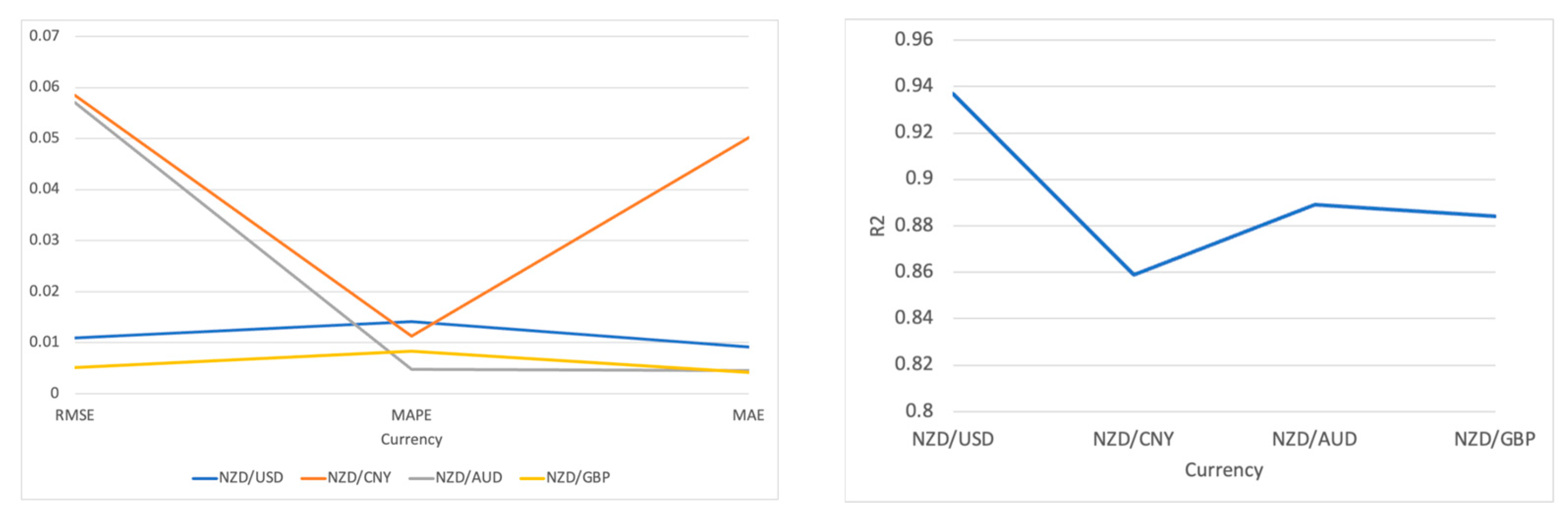
In summary, the Transformer performs outstandingly across all four datasets, especially in NZD/USD predictions, where it achieves a very high level of accuracy as shown in Figure 3.
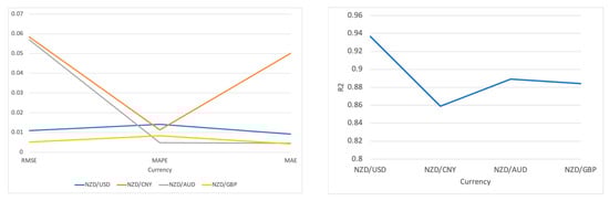
Figure 3.
Visualization of the experimental results on Transformer.
3.2. Experimental Results of Informer
The second model we conducted in this experiment was the Informer, an advancement based on the Transformer framework. The prediction trend in Figure 4 is as follows through the training and prediction of four datasets.

Figure 4.
The predictive results of each dataset performed by using Informer.
From the prediction trend in Figure 5, the actual and predicted values of NZD/USD are roughly similar, especially at the peaks and troughs. However, between July 2022 and January 2023, there is a relatively large gap between the predicted and actual lines. As for NZD/CNY, the overall prediction for this currency pair also maintained synchronicity, but the deviation at the beginning of 2023 was more extensive than that of NZD/USD. Similar to NZD/USD and NZD/AUD, where the prediction curve of this currency pair closely matches the actual price curve most of the time. Likewise, in a number of intervals, the prediction failed to capture the rapid changes in the exact exchange rate. Slightly different from the trend results of the other three, the trend of NZD/GBP did not match as well as the others, but it also captured the trend of the exchange rate. Table 2 illustrates the results based on the four evaluation metrics.
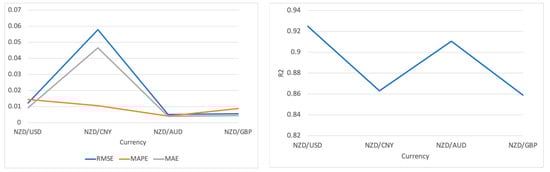
Figure 5.
Visualization of the experimental results on Informer.
Table 2.
The parameter settings of Transformer.
In the NZD/USD results, the Informer model achieved a high level of precision, specifically reflected in the low RMSE value 0.012. At the same time, the low MAPE and MAE values 0.0144 and 0.0092, respectively, also demonstrate that the forecast errors are relatively minor. An R2 value 0.925 further indicates that the Informer can broadly explain fluctuations in the exchange rate.
In the NZD/CNY results, despite the low MAPE value 0.0105, which explains a certain degree of accuracy, the higher RMSE and MAE values reveal the challenges faced by the Informer in predicting this currency pair. Nevertheless, an R2 value exceeding 0.85 means that the Informer can still fit the data reasonably well despite the difficulties.
Regarding NZD/AUD and NZD/GBP, the Informer performed exceptionally well, especially in NZD/AUD, where the very low RMSE and MAE values reflect the superior performance of the Informer model in terms of prediction accuracy. The MAPE value is nearly zero, almost achieving a perfect prediction effect. This shows that the Informer can accurately predict the exchange rate movements of these two currency pairs, even in the face of fluctuations in exchange rates.
Overall, the Informer model demonstrates adaptability and accuracy under different market conditions in handling the exchange rate predictions of these four datasets. Particularly in predicting NZD/AUD and NZD/USD, it illustrates the advantages of being an improved model based on the Transformer. Although there are challenges in the NZD/CNY predictions, the model can still effectively capture and predict the dynamics of exchange rate changes.
3.3. Experimental Results of TFT
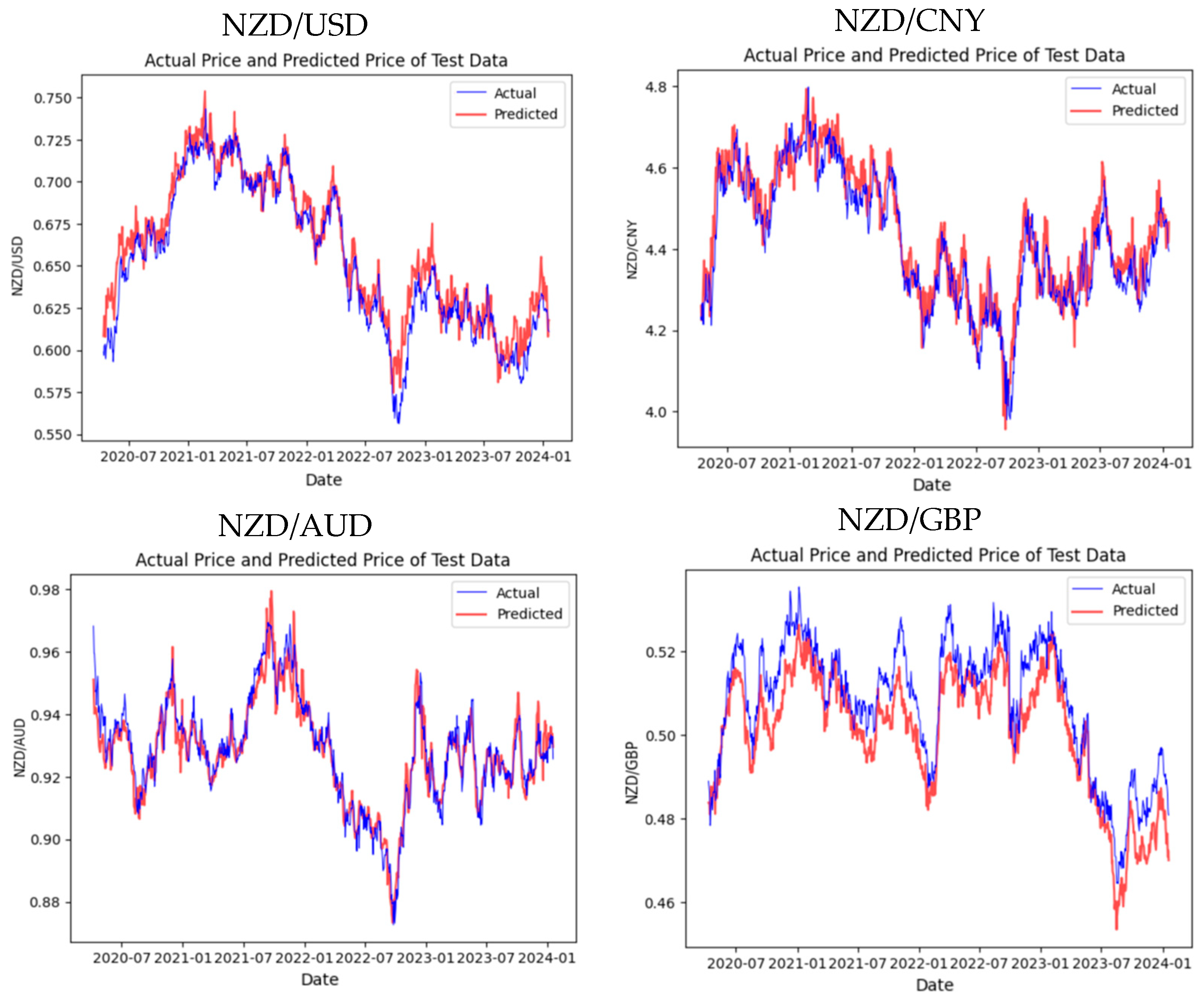
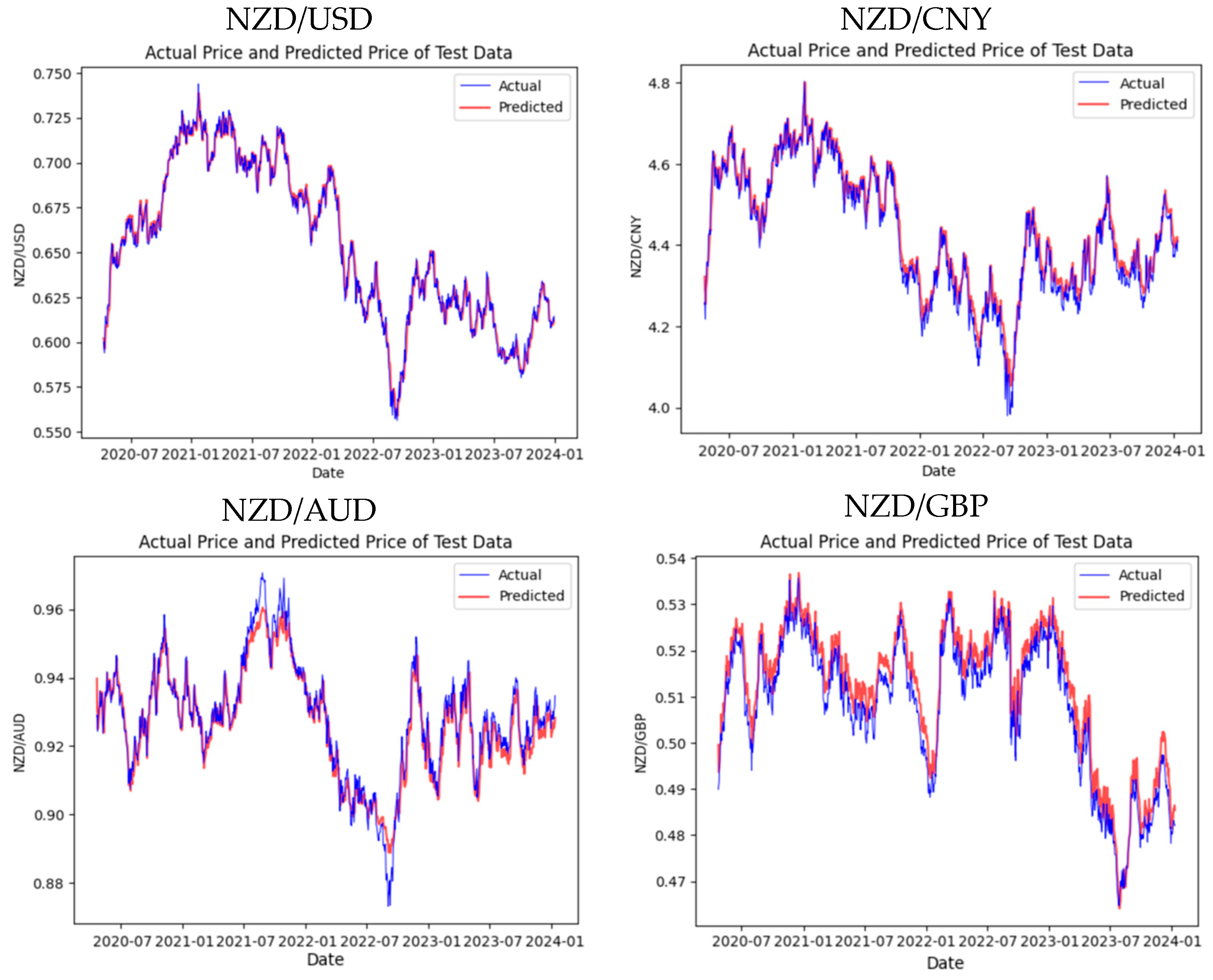
Our third trained model is the TFT, an enhancement of the Transformer model that specializes in processing time series data. Figure 6 exhibits the TFT’s prediction trends for the four test sets.

Figure 6.
The predictive results of each dataset performed on TFT.
From the trend chart of NZD/USD, the prediction curve closely follows the actual price curve most of the time, demonstrating the solid predictive capability of the TFT model for this currency pair, particularly in adapting quickly during significant trend changes. As for the trend charts of the other three currency pairs, we observe the lag or deviation at critical turning points. Nevertheless, the TFT model generally follows the actual trends well. Table 3 shows the result by using evaluation metrics.
Table 3.
The parameter settings of Informer.
The assessment results in Table 3 show that the predictions for NZD/USD are the best, with shallow RMSE, MAPE and MAE values 0.0045, 0.0055 and 0.0035, respectively, revealing that the predicted values are very close to the actual values. The high R2 value additionally confirms the nearness between the predicted and actual trends of exchange rate fluctuations for this currency pair.
As for the results of NZD/CNY, though the MAPE remains at a low level 0.0056, a relatively higher RMSE suggests significant deviations between the predicted and actual values at specific time points. However, the high R2 value 0.96 indicates that the TFT model can still capture most exchange rate changes.
In the predictions for NZD/AUD, even though the R2 value is slightly lower than that of NZD/USD, the remarkably low errors indicate the high accuracy of the TFT on this test set.
Although NZD/GBP has the highest MAE among all the currency pairs at 0.0075, this does not mean that the overall performance of this model is poor. An R2 value 0.9122 points out that the model successfully captures most of the dynamics of the pound’s exchange rate changes, with a slight decrease in predictive accuracy, possibly due to the complexity of market fluctuations during specific periods.
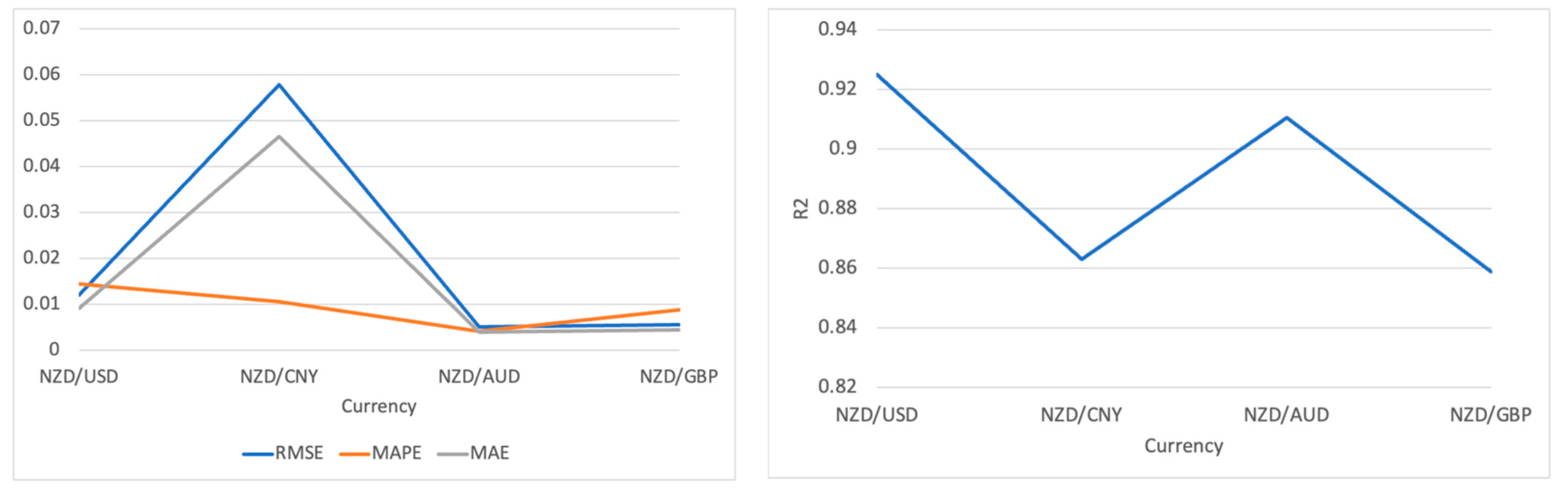
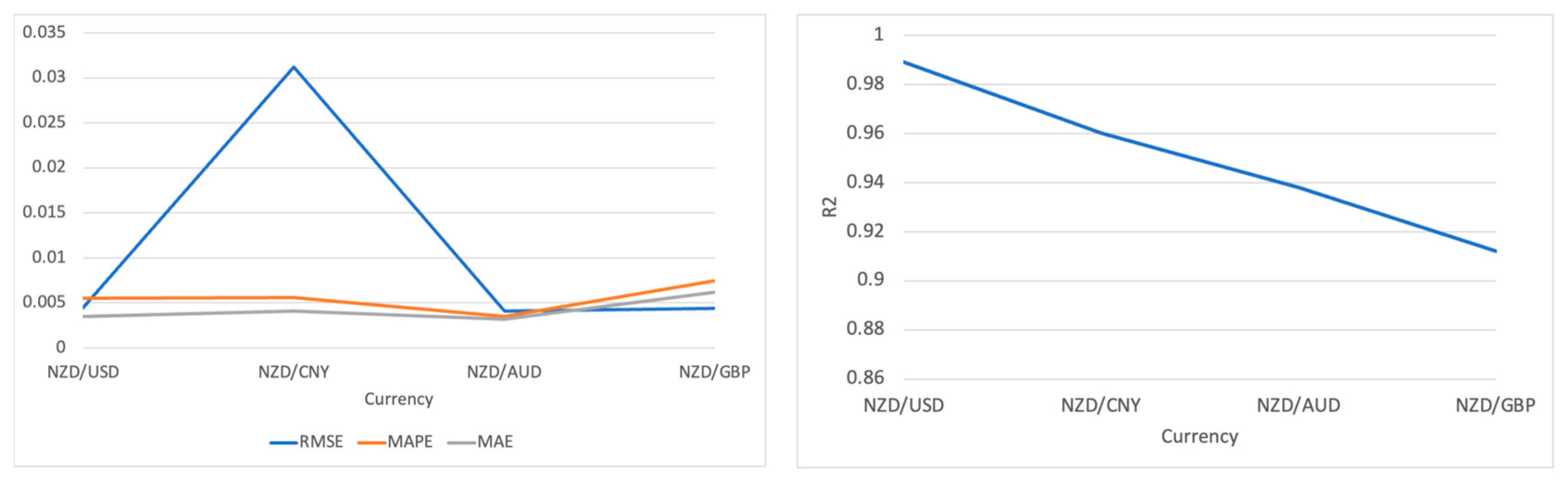
The TFT model performs reasonably well across all four test sets, especially in predicting NZD/USD and NZD/AUD, showing high accuracy and reliability. Despite the drop in predictive precision for NZD/CNY and NZD/GBP, the R2 values still demonstrate that the model’s predictions are pretty reliable for these currency pairs as shown in Figure 7.

Figure 7.
Visualization of the experimental results on TFT.
4. Analysis and Discussion
To compare the performance of these three models more thoroughly—Transformer, Informer, and TFT, we summarized the evaluation results of each model for the four test sets, taking the average for each evaluation criterion. The results are presented in Table 4.
Table 4.
The parameters setting of TFT.
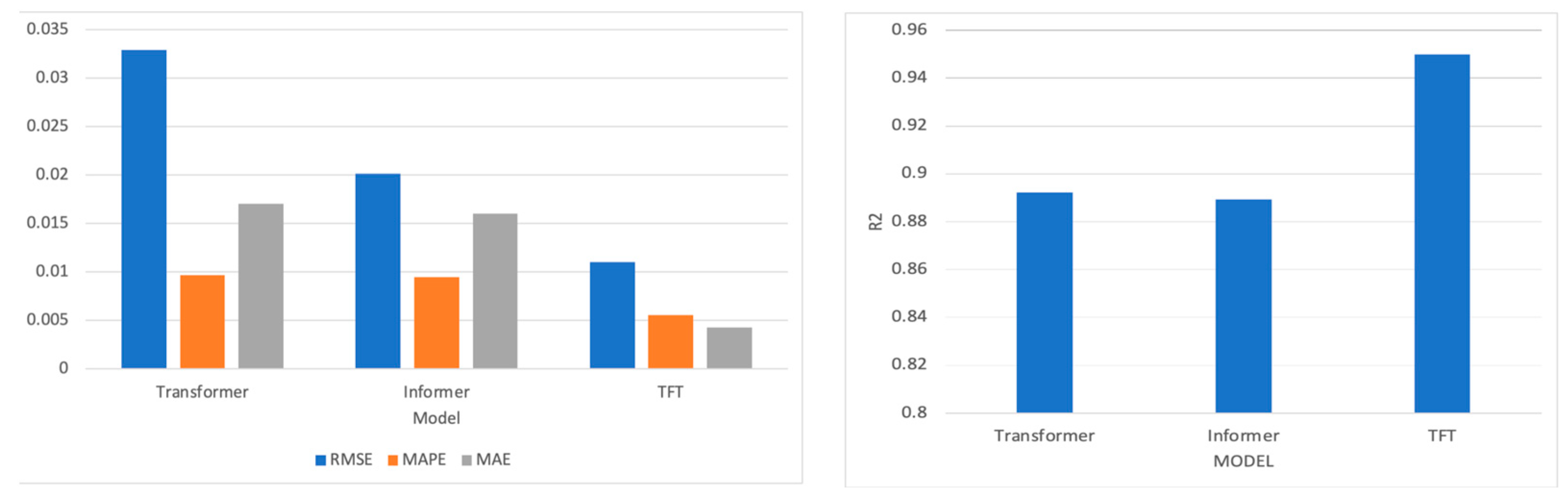
In Table 5, it is evident that the Transformer model has relatively high RMSE and MAE values. Nevertheless, an R2 value 0.8922 indicates a reasonable correlation between the predictions and actual values. Its explanatory power is slightly weaker compared to the other two models. As an improved version of the Transformer, the Informer has lower RMSE and MAE values in Table 6, at 0.0201 and 0.016, respectively, while its MAPE is 0.0095 and R2 is 0.8893. This suggests that the Informer performs better than the original Transformer, especially when dealing with time series data with high volatility. Lastly, the TFT exhibits the best performance among all the models in Table 7, with an RMSE of only 0.0111, a MAPE 0.0055, an MAE 0.0043, and the highest R2 value 0.9499. The TFT model integrates various methods for time series forecasting, including time attention mechanisms and interpretable features, enabling it to excel across all evaluation metrics in Table 8.
Table 5.
The experimental results with four datasets using Transformer.
Table 6.
The experimental results with four datasets by using Informer.
Table 7.
The TFT experiment results with four datasets.
Table 8.
The evaluation results of each model based on the test set.
As shown in Figure 8, these results imply that the TFT performs best in handling the currency exchange rate prediction, possibly because it was designed to capture complex patterns in time series. The Informer and Transformer also perform well but cannot achieve outstanding results like the TFT for this specific task. The differences may derive from the special treatment of the time dimension in its model architecture and its ability to capture and integrate various factors affecting the predictive variables.

Figure 8.
The visualization result of the three models’ performance.
Additionally, from the perspective of training time and model convergence speed, the Informer is able to reach stable and accurate predictions within a relatively few 60 epochs, which might make it more efficient than the traditional Transformer and the TFT. However, by considering the performance after model training, the TFT has demonstrated the highest R2 value in currency exchange rate predictions. Although the TFT might require a more complex training process, its return on investment in model performance is optimal.
5. Conclusions
This paper aims to analyze and discuss the accuracy and performance of models through exchange rate predictions. This paper makes use of three models: Transformer and its advanced versions, Informer and TFT. We collected four exchange rate datasets, namely, NZD/USD, NZD/CNY, NZD/GBP and NZD/AUD, and applied them to the three models for training and validation. Our experiments were conducted on the Google Colab platform, four evaluation criteria were utilized to analyze and compare the performance of the three models.
All three models achieved satisfactory prediction effects on the four datasets. However, comparisons indicated that the TFT model offered the best performance in exchange rate prediction, especially regarding accuracy and capturing trends in data changes. The Informer balanced efficiency and accuracy, demonstrating excellent predictive capabilities in fewer epochs. This is due to its sparse attention mechanism, which reduces computational complexity. Among the three models, the Transformer performed the least ideally, with relatively higher RMSE and MAE values and the lowest R2 value.
The limitations of this paper mainly fall into three parts. Firstly, the variables selected for this project are limited, only including primary exchange rate data. However, exchange rate trends are influenced by other complex factors, such as national policies, inflation rates, and investor psychological expectations. Thus, the lack of comprehensive feature selection will inevitably lead to unavoidable errors in prediction. Based on this, it is possible to consider incorporating more factors that affect exchange rates in the data selection process. Secondly, due to limited time, each model’s selection of parameters and functions was primarily based on relevant literature and materials, which may introduce subjectivity and randomness. Therefore, further research and experimentation are needed to select the optimal parameters. Thirdly, the experiments in this paper are all based on the Transformer model’s framework. It is vital to conduct experimental comparisons with other cutting-edge models to comprehensively analyze and determine the best model for predicting exchange rates.
Although this paper has made great progress in exchange rate prediction, numerous shortages and issues still require further investigation. Therefore, our future research work will be conducted in the following aspects. To enhance the accuracy of our models in predicting exchange rates, it is necessary to include more economic indicators and other relevant factors influencing exchange rates in the data collection process. Hence, further research work and experimental validation are required to optimize model parameters. In addition, we plan to expand the experimental data by using currencies from other representative countries as benchmarks for exchange rate prediction. We will also explore and compare more recent models to further enhance the effectiveness and accuracy of exchange rate forecasting, thereby providing valuable reference recommendations for the financial markets.
Author Contributions
Conceptualization, L.Z.; methodology, L.Z.; software, L.Z.; validation, L.Z.; formal analysis, L.Z.; investigation, L.Z.; resources, L.Z. and W.Q.Y.; data collection, L.Z.; writing—original draft preparation, L.Z.; writing—review and editing, L.Z.; supervision, W.Q.Y.; project administration W.Q.Y. All authors have read and agreed to the published version of the manuscript.
Funding
This research project has no external funding.
Data Availability Statement
Data are contained within the article.
Conflicts of Interest
The authors declare no conflicts of interest.
References
- Bi, Jiarui, Zengliang Zhu, and Qinglong Meng. 2021. Transformer in computer vision. Paper presented at 2021 IEEE International Conference on Computer Science, Electronic Information Engineering and Intelligent Control Technology (CEI), Fuzhou, China, September 24–26. [Google Scholar]
- Fayer, Geane, Larissa Lima, Felix Miranda, Jussara Santos, Renan Campos, Vinícius Bignoto, Marcel Andrade, Marconi Moraes, Celso Ribeiro, Priscila Capriles, and et al. 2023. A temporal fusion transformer deep learning model for long-term streamflow forecasting: A case study in the funil reservoir. Southeast Brazil. Knowledge-Based Engineering and Sciences 4: 73–88. [Google Scholar]
- Gong, Mingju, Yin Zhao, Jiawang Sun, Cuitian Han, Guannan Sun, and Bo Yan. 2022. Load forecasting of district heating system based on Informer. Energy 253: 124179. [Google Scholar] [CrossRef]
- Han, Kai, Yunhe Wang, Hanting Chen, Xinghao Chen, Jianyuan Guo, Zhenhua Liu, Yehui Tang, An Xiao, Chunjing Xu, Yixing Xu, and et al. 2022. A survey on vision transformer. IEEE Transactions on Pattern Analysis and Machine Intelligence 45: 87–110. [Google Scholar] [CrossRef] [PubMed]
- Hu, Zexin, Yiqi Zhao, and Matloob Khushi. 2021. A survey of forex and stock price prediction using deep learning. Applied System Innovation 4: 9. [Google Scholar] [CrossRef]
- Khashei, Mehdi, and Mehdi Bijari. 2011. A novel hybridization of artificial neural networks and ARIMA models for time series forecasting. Applied Soft Computing 11: 2664–75. [Google Scholar] [CrossRef]
- Lai, Guokun, Wei-Cheng Chang, Yiming Yang, and Hanxiao Liu. 2018. Modeling long-and short-term temporal patterns with deep neural networks. Paper presented at 41st International ACM SIGIR Conference on Research & Development in Information Retrieval, Ann Arbor, MI, USA, July 8–12; pp. 95–104. [Google Scholar]
- Lara-Benítez, Pedro, Luis Gallego-Ledesma, Manuel Carranza-García, and José M. Luna-Romera. 2021. Evaluation of the transformer architecture for univariate time series forecasting. Paper presented at 19th Conference of the Spanish Association for Artificial Intelligence, CAEPIA 2020/2021, Málaga, Spain, September 22–24. [Google Scholar]
- Li, Shuai, Wanqing Li, Chris Cook, Ce Zhu, and Yanbo Gao. 2018. Independently recurrent neural network (indrnn): Building a longer and deeper RNN. Paper presented at IEEE Conference on Computer Vision and Pattern Recognition, Salt Lake City, UT, USA, June 18–22. [Google Scholar]
- Lim, Bryan, Sercan Ö. Arık, Nicolas Loeff, and Tomas Pfister. 2021. Temporal fusion transformers for interpretable multi-horizon time series forecasting. International Journal of Forecasting 37: 1748–64. [Google Scholar] [CrossRef]
- Niu, Hongli, and Lin Zhang. 2017. Nonlinear multiscale entropy and recurrence quantification analysis of foreign exchange markets efficiency. Entropy 20: 17. [Google Scholar] [CrossRef] [PubMed]
- Pirani, Muskaan, Paurav Thakkar, Pranay Jivrani, Mohammed Husain Bohara, and Dweepna Garg. 2022. A comparative analysis of ARIMA, GRU, LSTM and BiLSTM on financial time series forecasting. Paper presented at IEEE International Conference on Distributed Computing and Electrical Circuits and Electronics (ICDCECE), Ballari, India, April 23–24. [Google Scholar]
- Pradeepkumar, Dadabada, and Vadlamani Ravi. 2018. Soft computing hybrids for FOREX rate prediction: A comprehensive review. Computers & Operations Research 99: 262–84. [Google Scholar]
- Rout, Ajit Kumar, Pradiptaishore Kishore Dash, Rajashree Dash, and Ranjeeta Bisoi. 2017. Forecasting financial time series using a low complexity recurrent neural network and evolutionary learning approach. Journal of King Saud University-Computer and Information Sciences 29: 536–52. [Google Scholar] [CrossRef]
- Sridhar, Sashank, and Sowmya Sanagavarapu. 2021. Multi-head self-attention transformer for dogecoin price prediction. Paper presented at International Conference on Human System Interaction (HSI), Gdańsk, Poland, July 8–10. [Google Scholar]
- Sun, Yuzhen, Lu Hou, Zhengquan Lv, and Daogang Peng. 2022. Informer-based intrusion detection method for network attack of integrated energy system. IEEE Journal of Radio Frequency Identification 6: 748–52. [Google Scholar] [CrossRef]
- Tay, Yi, Mostafa Dehghani, Dara Bahri, and Donald Metzler. 2022. Efficient transformers: A survey. ACM Computing Surveys 55: 1–28. [Google Scholar] [CrossRef]
- Vaswani, Ashish, Noam Shazeer, Niki Parmar, Jakob Uszkoreit, Llion Jones, Aidan N. Gomez, Łukasz Kaiser, and Illia Polosukhin. 2017. Attention is all you need. Paper presented at Advances in Neural Information Processing Systems 30., Long Beach, CA, USA, December 4–9. [Google Scholar]
- Wang, Xixuan, Dechang Pi, Xiangyan Zhang, Hao Liu, and Chang Guo. 2022. Variational transformer-based anomaly detection approach for multivariate time series. Measurement 191: 110791. [Google Scholar] [CrossRef]
- Wen, Qingsong, Tian Zhou, Chaoli Zhang, Weiqi Chen, Ziqing Ma, Junchi Yan, and Liang Sun. 2023. Transformers in time series: A survey. Paper presented at Thirty-Second International Joint Conference on Artificial Intelligence, Macao, China, August 19–25; pp. 6778–86. [Google Scholar]
- Wu, Haixu, Jiehui Xu, Jianmin Wang, and Mingsheng Long. 2021. Autoformer: Decomposition transformers with auto-correlation for long-term series forecasting. Advances in Neural Information Processing Systems 34: 22419–30. [Google Scholar]
- Xu, Yang, Liyan Han, Li Wan, and Libo Yin. 2019. Dynamic link between oil prices and exchange rates: A non-linear approach. Energy Economics 84: 104488. [Google Scholar] [CrossRef]
- Yamak, Peter T., Li Yujian, and Pius K. Gadosey. 2019. A comparison between arima, lstm, and GRU for time series forecasting. Paper presented at International Conference on Algorithms, Computing and Artificial Intelligence, Sanya, China, December 20–22. [Google Scholar]
- Yıldıran, Cenk Ufuk, and Abdurrahman Fettahoğlu. 2017. Forecasting USDTRY rate by ARIMA method. Cogent Economics & Finance 5: 1335968. [Google Scholar]
- Zhang, Hao, Yajie Zou, Xiaoxue Yang, and Hang Yang. 2022. A temporal fusion transformer for short-term freeway traffic speed multistep prediction. Neurocomputing 500: 329–40. [Google Scholar] [CrossRef]
- Zhou, Haoyi, Shanghang Zhang, Jieqi Peng, Shuai Zhang, Jianxin Li, Hui Xiong, and Wancai Zhang. 2021. Informer: Beyond efficient transformer for long sequence time-series forecasting. Paper presented at AAAI Conference on Artificial Intelligence, Virtually, February 2–9. [Google Scholar]
Disclaimer/Publisher’s Note: The statements, opinions and data contained in all publications are solely those of the individual author(s) and contributor(s) and not of MDPI and/or the editor(s). MDPI and/or the editor(s) disclaim responsibility for any injury to people or property resulting from any ideas, methods, instructions or products referred to in the content. |
© 2024 by the authors. Licensee MDPI, Basel, Switzerland. This article is an open access article distributed under the terms and conditions of the Creative Commons Attribution (CC BY) license (https://creativecommons.org/licenses/by/4.0/).