Segmental Track Analysis in Dynamic Wireless Power Transfer

 , ,
, ,
Abstract
:
1. Introduction
2. Dynamic Charging System Circuit Model Analysis
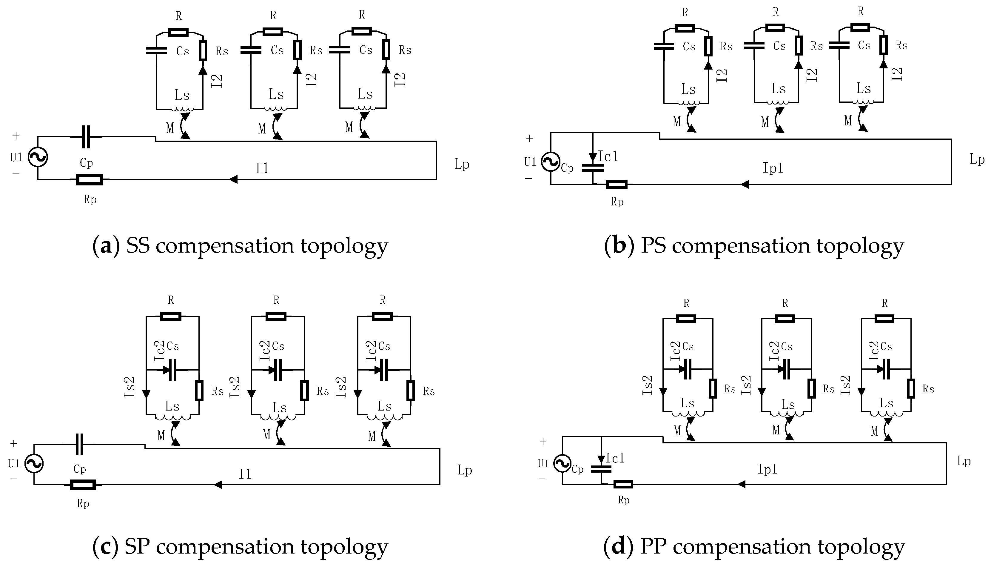
2.1. Basic Compensation Topologies
2.2. Equivalent Circuit Model Analysis
3. Simulation Analysis and Track Length Plan Algorithm
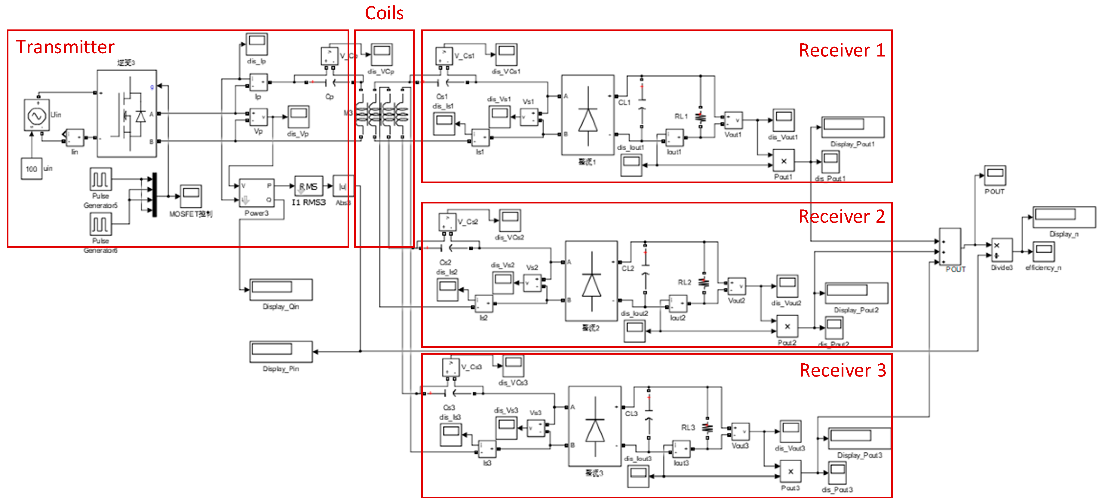
3.1. Circuit Simulation and Analysis
3.2. Magnetic Field Simulation and Analysis
3.2.1. Track Length Analysis with Single Receiving Coil
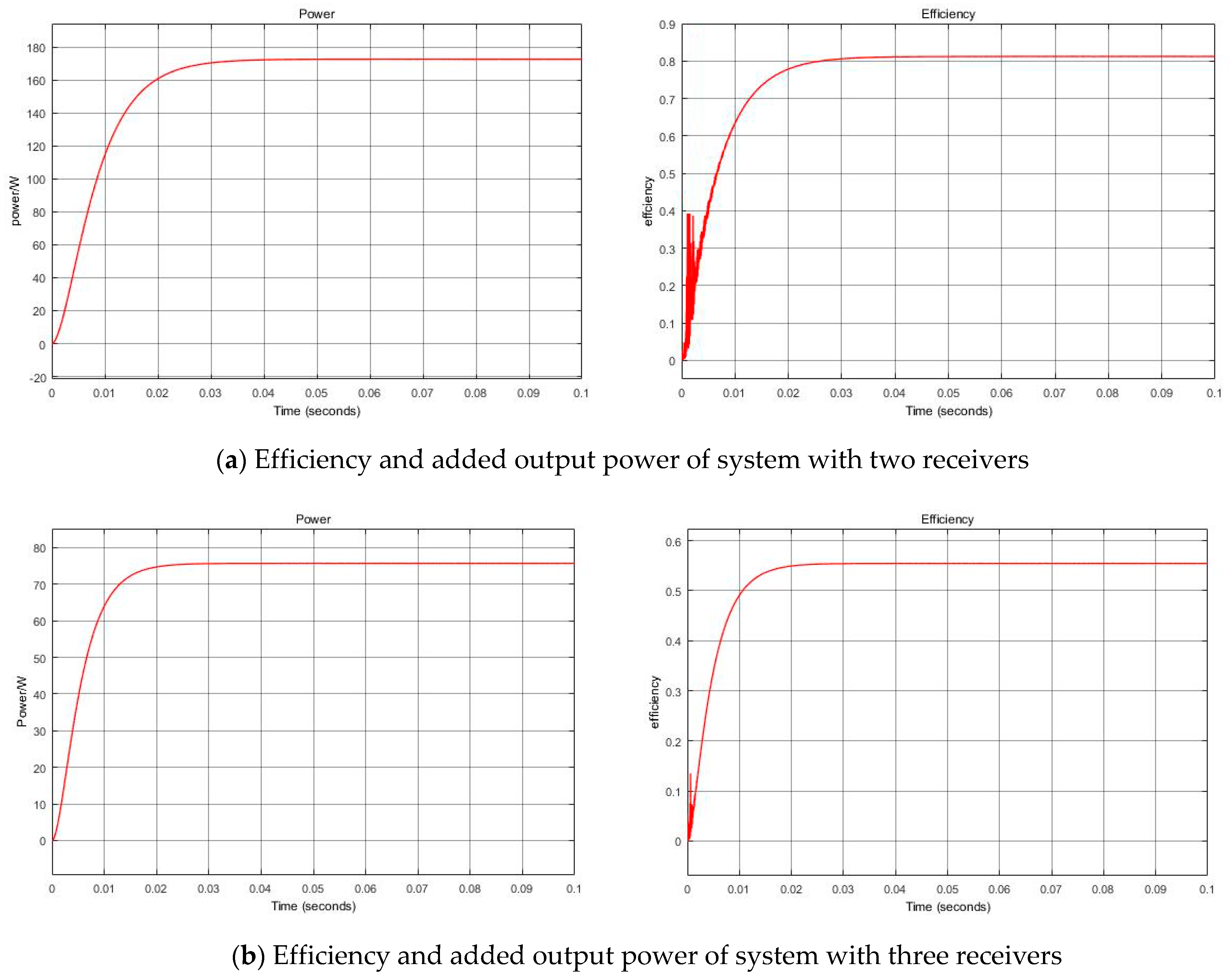
3.2.2. Track Length Analysis with Multi Receiving Coils
4. Experimental Verification
5. Conclusions
Author Contributions
Funding
Conflicts of Interest
References
- Li, S.; Liu, Z.; Zhao, H.; Zhu, L.; Shuai, C.; Chen, Z. Wireless Power Transfer by Electric Field Resonance and Its Application in Dynamic Charging. IEEE Trans. Ind. Electron. 2016, 63, 6602–6612. [Google Scholar] [CrossRef]
- Budhia, M.; Boys, J.T.; Covic, G.A.; Huang, C. Development and evaluation of single sided flux couplers for contactless electric vehicle charging. In Proceedings of the Energy Conversion Congress and Exposition, Phoenix, AZ, USA, 17–22 September 2011. [Google Scholar]
- Zhou, S.; Mi, C.C. Multi-Paralleled LCC Reactive Power Compensation Networks and Their Tuning Method for Electric Vehicle Dynamic Wireless Charging. IEEE Trans. Ind. Electron. 2016, 63, 6546–6556. [Google Scholar] [CrossRef]
- Zhang, Z.; Pang, H.; Lee, C.H.T.; Xu, X.; Wei, X.; Wang, J. Comparative Analysis and Optimization of Dynamic Charging Coils for Roadway-Powered Electric Vehicles. IEEE Trans. Magn. 2017, 53. [Google Scholar] [CrossRef]
- Buja, G.; Bertoluzzo, M.; Dashora, H.K. Lumped Track Layout Design for Dynamic Wireless Charging of Electric Vehicles. IEEE Trans. Ind. Electron. 2016, 63, 6631–6640. [Google Scholar] [CrossRef]
- Zhang, Q.; Huang, Y.X.; Niu, T.; Xu, C. Analysis and Control of Dynamic Wireless Charging Output Power for Electric Vehicle. In Proceedings of the International Conference on Intelligent Computation Technology and Automation, Changsha, China, 9–10 September 2017. [Google Scholar]
- Deng, Q.; Liu, J.; Czarkowski, D.; Bojarski, M.; Chen, J.; Hu, W.; Zhou, H. Edge Position Detection of On-line Charged Vehicles with Segmental Wireless Power Supply. IEEE Trans. Veh. Technol. 2017, 66, 3610–3621. [Google Scholar]
- Tian, Y. Research on Key Sectional Track-Based Wireless Power Supply Technology for Electric Vehicles; Chongqing University: Chongqing, China, 2012. [Google Scholar]
- Lu, F.; Zhang, H.; Hofmann, H.; Mi, C.C. A Dynamic Charging System with Reduced Output Power Pulsation for Electric Vehicles. IEEE Trans. Ind. Electron. 2016, 63, 6580–6590. [Google Scholar] [CrossRef]
- Huh, J.; Lee, S.W.; Lee, W.Y.; Cho, G.H.; Rim, C.T. Narrow-width inductive power transfer system for online electric vehicles. IEEE Trans. Power Electron. 2011, 26, 3666–3679. [Google Scholar] [CrossRef]
- Su, Y.C.; Jeong, S.Y.; Gu, B.W.; Lim, G.C.; Rim, C.T. Ultraslim S-type power supply rails for roadway-powered electric vehicles. IEEE Trans. Power Electron. 2015, 30, 6456–6468. [Google Scholar]
- Park, C.; Lee, S.; Jeong, S.Y.; Cho, G.H. Uniform power I-type inductive power transfer system with DQ power supply rails for on-line electric vehicles. IEEE Trans. Power Electron. 2015, 30, 6446–6455. [Google Scholar] [CrossRef]
- Mi, C.C.; Buja, G.; Su, Y.C.; Rim, C.T. Modern Advances in Wireless Power Transfer Systems for Roadway Powered Electric Vehicles. IEEE Trans. Ind. Electron. 2016, 63, 6533–6545. [Google Scholar] [CrossRef]
- Choi, S.; Huh, J.; Lee, W.Y.; Lee, S.W.; Rim, C.T. New Cross-Segmented Power Supply Rails for Roadway-Powered Electric Vehicles. IEEE Trans. Power Electron. 2013, 28, 5832–5841. [Google Scholar] [CrossRef]
- Yilmaz, T.; Hasan, N.; Zane, R.; Pantic, Z. Multi-Objective Optimization of Circular Magnetic Couplers for Wireless Power Transfer Applications. IEEE Trans. Magn. 2017, 53, 1–12. [Google Scholar] [CrossRef]
- Zhang, W.; Wong, S.C.; Tse, C.K.; Chen, Q. An Optimized Track Length in Roadway Inductive Power Transfer Systems. IEEE J. Emerg. Sel. Top. Power Electron. 2014, 2, 598–608. [Google Scholar] [CrossRef]
- Wang, C.S.; Covic, G.; Stielau, O.H. Power Transfer Capability and Bifurcation Phenomena of Loosely Coupled Inductive Power Transfer Systems. IEEE Trans. Ind. Electron. 2004, 51, 148–157. [Google Scholar] [CrossRef]
- Villa, J.L.; Sallan, J.; Osorio, J.F.S.; Llombart, A. High-Misalignment Tolerant Compensation Topology for ICPT Systems. IEEE Trans. Ind. Electron. 2012, 59, 945–951. [Google Scholar] [CrossRef]
- Okada, K.; Iimura, K.; Hoshi, N.; Haruna, J. Comparison of two kinds of compensation schemes on inductive power transfer systems for electric vehicle. In Proceedings of the Vehicle Power & Propulsion Conference, Seoul, Korea, 9–12 October 2012; pp. 766–771. [Google Scholar]
- Bosshard, R.; Kolar, J.W.; Muhlethaler, J.; Stevanovic, I. Modeling and η-α-Pareto Optimization of Inductive Power Transfer Coils for Electric Vehicles. IEEE J. Emerg. Sel. Top. Power Electron. 2015, 3, 50–64. [Google Scholar] [CrossRef]


| Parameter | Value |
|---|---|
| Input voltage/ | 100 V |
| Resonant frequency/ | 100 kHz |
| Coupling coefficient between transmitter and receivers/ | 0.1 |
| Self-inductance of transmitting coil/ | 120 μH |
| Primary compensation capacitance/ | 21.1 nF |
| Self-inductance of receiving coils/ | 120 μH |
| Secondary compensation capacitance/ | 21.1 nF |
| Secondary quality factor/ | 6 |
| Load resistance/ | 2 Ω |
| /mm | /mm | |||||
|---|---|---|---|---|---|---|
| 150 | 10 | 6 | 3 | 50 | 6 | 2 |

| Parameter | 4dracetrack | 6dracetrack |
|---|---|---|
| Coupling coefficient between track and receiving coil 1/ | 0.1092 | 0.09044 |
| Coupling coefficient between track and receiving coil 2/ | 0.1098 | 0.08574 |
| Coupling coefficient between track and receiving coil 3/ | - | 0.09044 |
| Coupling coefficient between adjacent receiving coils | 0.004620 | 0.003797 |
| Sum of coupling coefficient of receiving coils | 0.2190 | 0.26662 |
| Parameter | Value |
|---|---|
| Input voltage | 10 V |
| Operating frequency | 100 kHz |
| Inductance of receiving coil | 17.5 μH |
| Inductance of 2d racetrack | 17 μH |
| Inductance of 2d rectangle | 19 μH |
| Inductance of 3d racetrack | 24.3 μH |
| Inductance of 3d rectangle | 26 μH |
| Resistance | 10 Ω |
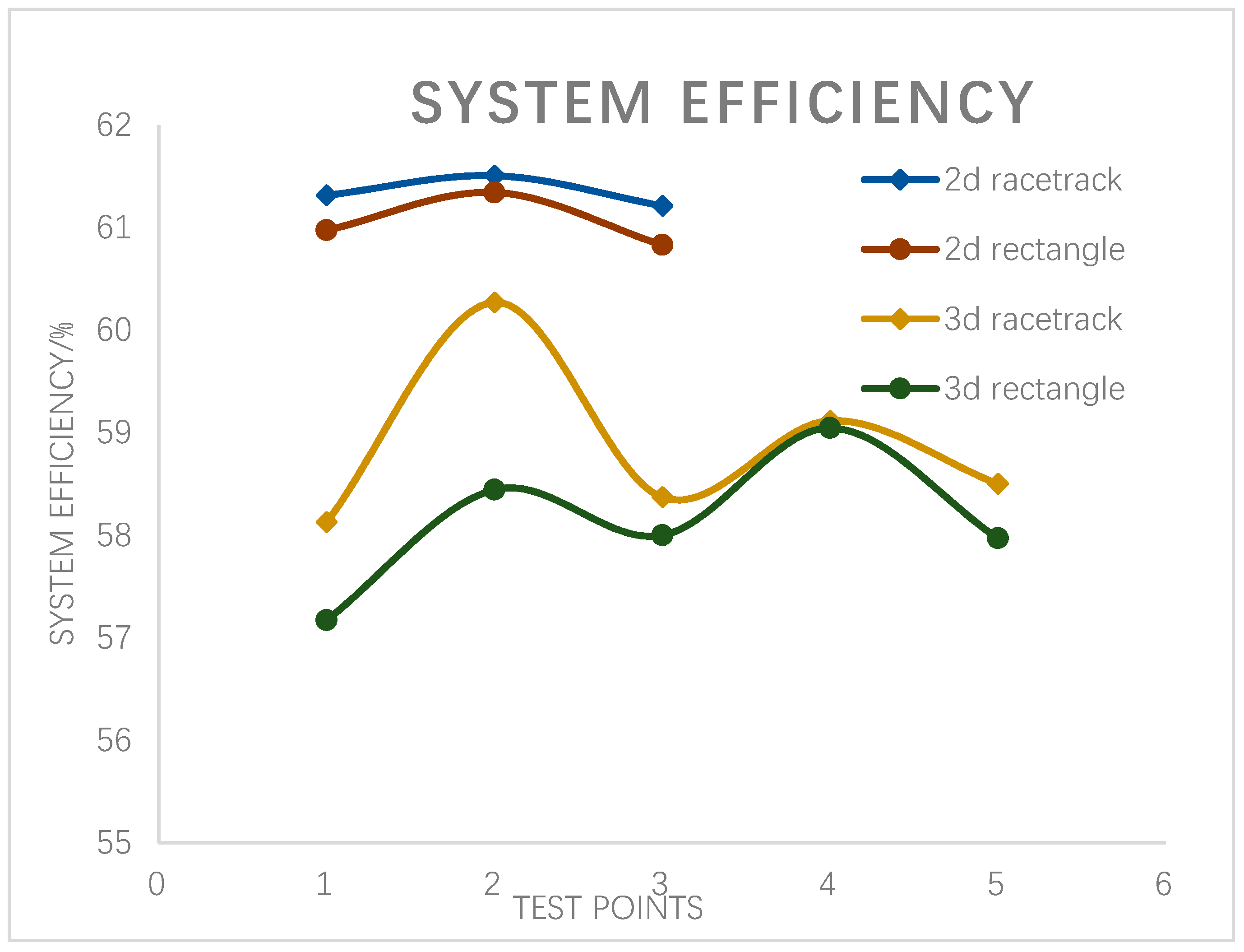
| Parameter | Primary Voltage/V | Primary Current/A | Input Power/W | Secondary Voltage/V | Secondary Current/A | Output Power/W | System Efficiency/% |
|---|---|---|---|---|---|---|---|
| 2d racetrack | 10 | 4.02 | 40.2 | 16.11 | 1.53 | 24.6483 | 61.3142 |
| 10 | 4.19 | 41.9 | 16.52 | 1.56 | 25.7712 | 61.5064 | |
| 10 | 4.41 | 44.1 | 16.46 | 1.64 | 26.9944 | 61.2118 | |
| 3d racetrack | 10 | 4.28 | 42.8 | 16.26 | 1.53 | 24.8778 | 58.1257 |
| 10 | 4.26 | 42.6 | 16.25 | 1.58 | 25.675 | 60.27 | |
| 10 | 4.53 | 45.3 | 16.63 | 1.59 | 26.4417 | 58.3702 | |
| 10 | 4.54 | 45.4 | 16.67 | 1.61 | 26.8387 | 59.1161 | |
| 10 | 4.84 | 48.4 | 17.16 | 1.65 | 28.314 | 58.5 | |
| 2d rectangle | 10 | 6.3 | 63 | 18.83 | 2.04 | 38.4132 | 60.9733 |
| 10 | 5.9 | 59 | 18.56 | 1.95 | 36.192 | 61.3424 | |
| 10 | 5.9 | 59 | 18.5 | 1.94 | 35.89 | 60.8305 | |
| 3d rectangle | 10 | 4.82 | 48.2 | 17.01 | 1.62 | 27.5562 | 57.1705 |
| 10 | 4.69 | 46.9 | 16.92 | 1.62 | 27.4104 | 58.4443 | |
| 10 | 4.92 | 49.2 | 17.19 | 1.66 | 28.5354 | 57.9988 | |
| 10 | 4.63 | 46.3 | 16.875 | 1.62 | 27.3375 | 59.0443 | |
| 10 | 4.67 | 46.7 | 16.92 | 1.6 | 27.072 | 57.97 |
© 2019 by the authors. Licensee MDPI, Basel, Switzerland. This article is an open access article distributed under the terms and conditions of the Creative Commons Attribution (CC BY) license (http://creativecommons.org/licenses/by/4.0/).
Share and Cite
Yang, S.-C.; He, H.; Yan, X.-Y.; Chen, Y.-H.; Hua, Y.; Cao, Y.-G.; Li, J.; Li, H.-H.; Yin, S. Segmental Track Analysis in Dynamic Wireless Power Transfer. Energies 2019, 12, 3875. https://doi.org/10.3390/en12203875
Yang S-C, He H, Yan X-Y, Chen Y-H, Hua Y, Cao Y-G, Li J, Li H-H, Yin S. Segmental Track Analysis in Dynamic Wireless Power Transfer. Energies. 2019; 12(20):3875. https://doi.org/10.3390/en12203875
Chicago/Turabian StyleYang, Shi-Chun, Hong He, Xiao-Yu Yan, Yu-Hang Chen, Yang Hua, Yao-Guang Cao, Jun Li, Hong-Hai Li, and Sheng Yin. 2019. "Segmental Track Analysis in Dynamic Wireless Power Transfer" Energies 12, no. 20: 3875. https://doi.org/10.3390/en12203875