Analysis and Exploitation of the Star-Point Voltage of Synchronous Machines for Sensorless Operation

Abstract

In the field of sensorless drive of synchronous machines (SMs), many techniques have been proposed that can be applied successfully in most applications. Nevertheless, these techniques rely on the measurement of the phase currents to extract the rotor position information. In the particular case of low-power machines, the application of such techniques is challenging due to the limited bandwidth of the available current sensors. An alternative is offered by those techniques that exploit the star-point voltage rather than phase currents. This work aims at providing a model of the dynamic behavior of the star-point voltage and presenting a technique for extracting the rotor electrical position needed for sensorless operation of SMs. Two different circuitries for measuring the star-point voltage are also presented and then compared. The presented mathematical analysis and the measurement methods are validated both numerically and experimentally on a test machine.

1. Introduction

In the field of electrical drives, there is an increasing demand for highly integrated and compact driving solutions where performance is preserved or improved while costs and size are minimized. In order to pursue such features, DC motors tend to be replaced in most application fields by synchronous motors (SMs) in advanced drive systems, such as permanent magnet synchronous motors (PMSMs), synchronous reluctance motors (SRMs) as well as PM-assisted synchronous reluctance motors (PM-SRMs).

To drive these machines, position information is required. Position sensors are typically installed for operating SMs, such as resolvers or encoders, which lead to an increase in cost, space requirement, and system complexity. It is, therefore, desirable to provide techniques, which allow the operation of SMs without having to resort to the use of position sensors. To address this problem, a significant number of scientific contributions have been published over the past few decades. The proposed sensorless techniques rely mainly on the exploitation of two physical effects: induced back-EMF (electro motive force) and the presence of machine anisotropies.

The first approaches to sensorless driving of SMs were based on the exploitation of the back-EMF signal, whose voltage is proportional to the rotor speed. By measuring the phase voltages and currents, the angular position can be either obtained by applying model reference adaptive system techniques (MRAS) or observed by means of state observers, such as Luenberger observers, sliding mode observers, and Kalman Filters. The main disadvantage of back-EMF based sensorless techniques is their inapplicability at low speeds and/or standstill conditions. This limitation incited a new field of techniques that can perform over the whole speed range by exploiting the presence of machine anisotropies. In particular, the dependence of the phase inductances on the rotor position has been investigated.

The very first attempt was proposed by Schroedl in [1,2]. In his papers, he proposes the basic theory of a sensorless technique that he refers to as INFORM (INdirect Flux-detection by Online Reactance Measurement). As the name indicates, INFORM allows online measurement of the motor reactances by means of current measurements resulting from the injection of test pulses based on the utilization of a modified pulse width modulation (PWM) driving signal. It is important to remark that the majority of motors exhibit a dependence of the phase reactances on the rotor position because of the nonlinear effects including hysteresis of the stator’s soft magnetic material as well as reluctance variations and saturation effects.

Right after the work of Schroedl, a scientific contribution was presented by Lorenz [3], who proposed a new way of modeling the dependence of the machine’s coil inductance on the rotor position under high-frequency excitation. In fact, in this work, the authors introduce the concept of leakage inductances by providing a simplified explanation of the physical behavior of motor phases under high-frequency excitation. Within the same work, the authors introduce a new approach to performing sensorless operations based on the injection of a rotating carrier. The currents induced by the carrier are modulated by the rotor position. Therefore, demodulation and state observation are necessary to extract the position information.

In [4] a new injection technique based on an alternating carrier was proposed. Such injection is performed in the estimated rotor reference frame with the direct advantage of reducing the computational effort necessary for extracting the rotor information. In particular, a pulsating voltage vector is introduced along the q-axis of the estimated rotor reference frame. Also in this case, this technique requires an observer that is dependent on the motor parameters.

As injecting an alternating carrier has been proven to be generally more efficient than using a rotating carrier in terms of precision, applicability, versatility, and robustness, most of the scientific works following the work of [5] have focused either on alternating carrier injection or on other arbitrary injection schemes [6,7,8,9].

By considering the scientific works mentioned above, it is therefore possible to distinguish the machine anisotropy based sensorless techniques between INFORM and high-frequency current injection (HFCI), the latter of which are based either on rotating, alternating or arbitrary carrier excitation. The most recent works in the field of sensorless operation aim at increasing the modeling precision necessary for performing sensorless operations, thus reducing the position estimation errors, and at the same time performing machine parameter identification, such as in the works [10,11]. New approaches combine sensorless operation with parameter identification to address the topic of the so-called self-commissioning [12].

All of the above mentioned sensorless techniques have the usage of current signal information in common. Nevertheless, current sensors are typically characterized by low signal-to-noise ratio, low sensitivity, and limited bandwidth. Such limitations directly affect the performance of current measurement based sensorless techniques, especially in the case of low-power electromagnetic motors. In fact, the sensorless techniques presented up to this point have been primarily tested on middle to high power machines. Nevertheless, low-power SMs are more challenging in terms of quality of the sensory information given that the driving currents are smaller and with larger bandwidth, clearly representing a limitation for such techniques. The main issues related to low-power PMSMs reside in the necessary higher frequency voltage switching (due to the small values of the inductances) and to the limited bandwidth of current sensors which, in this case, need to operate at higher frequencies.

In the particular case of star-connected SMs with accessible star points, current measurements can be avoided for sensorless operation by measuring the voltage of the motor star point that can deliver the necessary information for the online determination of the motor inductances. A thorough investigation has already been conducted and published in [13]. Nevertheless, a previous technique was first proposed in [14] and it is based on measuring the voltage difference between the machine star-point and a virtual star-point. Such a technique has been then elaborated and proposed in the scientific community from different authors and under different names, such as VirtuHall, Direct Flux Control, and Direct Flux Observer. The first scientific works were those of Thiemann [15] and Mantala [16], who proposed approaches to excite the machine to get meaningful signals and techniques for extracting the position information. In [17] an improved approach to the extraction of the position has been presented that reduces the presence of harmonics. To improve the quality of the measurements, a fast resettable integrator circuit (FRIC) was firstly proposed in [18,19].

The mentioned works concerning the usage of the machine star-point for sensorless operation have focused in particular on PMSMs with assumptions on the inductance matrix and, therefore, the nature of the measured signals. In this work, a new mathematical model of the star-point voltage is proposed to analyze the measured signals in relation to any kind of synchronous machine. The dynamic response of the machine star-point to the terminal voltage excitations is also presented. This paper is divided into three sections. In the first one, the mathematical description of the star-point voltage dynamic is presented. As it is necessary to measure the star-point, the effect of a measuring impedance is also taken into account. Furthermore, a method to extract information about the machine inductances, as well as the position information from the voltage difference between the machine star-point and a virtual star-point, is described. In the second section, two different methods for measuring the star-point voltage are presented: direct voltage measurement and fast resettable integrator circuit. Finally, in the third section, experimental results are presented and discussed to confirm the theoretical analysis discussed in the previous sections.

2. Mathematical Model

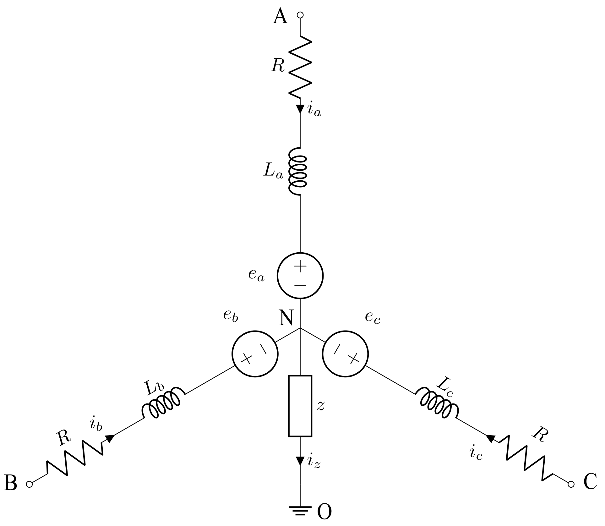
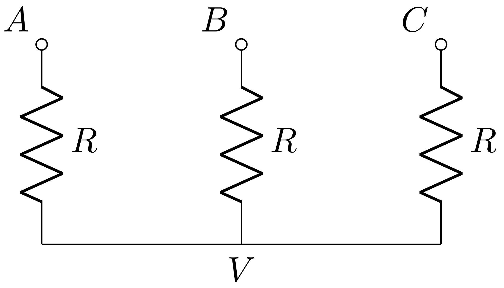
This section aims at presenting the mathematical description of the dynamic behavior of the machine star-point voltage within a PWM time period and proposes a technique to extract information about the machine phase inductances. Let us consider the electrical equation of a three-phase synchronous machine as depicted in Figure 1:

$${\mathbf{v}}_{abc}\left(t\right)=\mathbf{R}{\mathbf{i}}_{abc}\left(t\right)+\frac{\mathrm{d}}{\mathrm{d}t}\left[{\mathbf{L}}_{abc}\left(t\right){\mathbf{i}}_{abc}\left(t\right)\right]+{\omega }_r\left(t\right)\mathbf{e}\left(t\right),$$

(1)

where $\mathbf{R}$ is the resistance matrix, ${\mathbf{L}}_{abc}$ is the inductance matrix, ${\omega }_r$ is the electrical rotor speed, ${\mathbf{v}}_{abc}={\left[\begin{array}{ccc}{v}_{AO}& v_{BN}& v_{CN}\end{array}\right]}^T$ and ${\mathbf{i}}_{abc}={\left[\begin{array}{ccc}{i}_a& i_b& i_c\end{array}\right]}^T$ are, respectively, voltages and current vectors of the phases $A,B,C$, and $\mathbf{e}$ is defined as follows:

$$\mathbf{e}\left(t\right)=-{\lambda }_{PM}\left[\begin{array}{c}sin\left({\theta }_r\left(t\right)\right)\\ sin({\theta }_r\left(t\right)-\frac{2}{3}\pi )\\ sin({\theta }_r\left(t\right)-\frac{4}{3}\pi )\end{array}\right]=\left[\begin{array}{c}{e}_a\\ e_b\\ e_c\end{array}\right],$$

(2)

where ${\theta }_r$ is the electrical rotor position and ${\lambda }_{PM}$ is the back-EMF constant.

Figure 1. The electrical equivalent circuit of a synchronous machine (SM) with a generic impedance connected to the star-point.

Let us assume that ${\mathbf{L}}_{abc}$ is a function of ${\theta }_r$ and that it is invertible per each value of ${\theta }_r$. One can write the electrical equation as follows:

$${\mathbf{v}}_{abc}=\mathbf{R}{\mathbf{i}}_{abc}+{\mathbf{L}}_{abc}\frac{\mathrm{d}}{\mathrm{d}t}{\mathbf{i}}_{abc}+{\omega }_r\frac{\partial {\mathbf{L}}_{abc}}{\partial {\theta }_r}{\mathbf{i}}_{abc}+{\omega }_r\mathbf{e},$$

(3)

where the time dependency notation “$\left(t\right)$” has been neglected.

2.1. Dynamic Behaviour of the Star-Point Voltage

As this analysis is intended to model the dynamics of the star-point voltage within one PWM period, the back-EMF and the machine phase inductances are considered constant. In fact, the PWM frequency is chosen much higher than the electrical and mechanical frequencies of the machine. Thus, ${\mathbf{L}}_{abc}$, $\mathbf{e}$ and ${\omega }_r$ are treated as time-independent quantities. Let us apply the Laplace transform to (3):

$${\mathbf{V}}_{abc}\left(s\right)=\mathbf{R}{\mathbf{I}}_{abc}\left(s\right)+{\mathbf{L}}_{abc}s{\mathbf{I}}_{abc}\left(s\right)-{\mathbf{L}}_{abc}{\mathbf{i}}_{abc}\left(0^{-}\right)+{\omega }_r\frac{\partial {\mathbf{L}}_{abc}}{\partial {\theta }_r}{\mathbf{I}}_{abc}\left(s\right)+\frac{{\omega }_r\mathbf{e}}{s},$$

(4)

that can be rewritten as

$$s{\mathbf{I}}_{abc}={\mathbf{L}}_{abc}^{-1}{\mathbf{V}}_{abc}-{\mathbf{L}}_{abc}^{-1}\mathbf{R}{\mathbf{I}}_{abc}+{\mathbf{L}}_{abc}^{-1}{\mathbf{L}}_{abc}{\mathbf{i}}_{abc}\left(0^{-}\right)-{\omega }_r{\mathbf{L}}_{abc}^{-1}\frac{\partial {\mathbf{L}}_{abc}}{\partial {\theta }_r}{\mathbf{I}}_{abc}-\frac{{\omega }_r{\mathbf{L}}_{abc}^{-1}\mathbf{e}}{s},$$

(5)

where ${\mathbf{L}}_{abc}^{-1}{\mathbf{L}}_{abc}$ has not been simplified for convenience and s-dependence has been neglected. Let us express ${\mathbf{L}}_{abc}^{-1}$ as ${\mathbf{L}}_{abc}^{-1}=\frac{{\mathbf{L}}_{abc}^{*}}{\left|{\mathbf{L}}_{abc}\right|}$, where ${\mathbf{L}}_{abc}^{*}$ is the adjoint matrix of ${\mathbf{L}}_{abc}$. Therefore, (5) can be written as

$$s{\mathbf{I}}_{abc}=\frac{{\mathbf{L}}_{abc}^{*}}{\left|{\mathbf{L}}_{abc}\right|}{\mathbf{V}}_{abc}-\frac{{\mathbf{L}}_{abc}^{*}}{\left|{\mathbf{L}}_{abc}\right|}\mathbf{R}{\mathbf{I}}_{abc}+\frac{{\mathbf{L}}_{abc}^{*}}{\left|{\mathbf{L}}_{abc}\right|}{\mathbf{L}}_{abc}{\mathbf{i}}_{abc}\left(0^{-}\right)-{\omega }_r\frac{{\mathbf{L}}_{abc}^{*}}{\left|{\mathbf{L}}_{abc}\right|}\frac{\partial {\mathbf{L}}_{abc}}{\partial {\theta }_r}{\mathbf{I}}_{abc}-{\omega }_r\frac{{\mathbf{L}}_{abc}^{*}}{\left|{\mathbf{L}}_{abc}\right|}\mathbf{e}\frac{1}{s}.$$

(6)

Let us now consider a generic impedance z connected between the machine star-point and ground, whose voltage is indicated as $v_{NO}$ and the current $i_z$ flowing through it is considered positive in the direction from star-point to ground. Also, the impedance is supposed to be constant. Thus, we can define the transfer function relative to the impedance as $Z\left(s\right)=\frac{V_{NO}\left(s\right)}{I_z\left(s\right)}$. According to Kirchhoff laws, one can write

$$\sum _{k=a,b,c}{i}_k=i_z,\sum _{k=a,b,c}\frac{\mathrm{d}}{\mathrm{d}t}{i}_k=\frac{\mathrm{d}}{\mathrm{d}t}{i}_z,$$

(7)

leading to the following equations in the Laplace domain:

$$\sum _{k=a,b,c}{I}_k\left(s\right)=I_z\left(s\right),\sum _{k=a,b,c}s{I}_k\left(s\right)=s{I}_z\left(s\right).$$

(8)

Let us define the row vector $\mathbf{T}=\left[\begin{array}{ccc}1& 1& 1\end{array}\right]$ and multiply (6) on the left by the vector $\mathbf{T}$. One can write

$$s\mathbf{T}{\mathbf{I}}_{abc}=\mathbf{T}\frac{{\mathbf{L}}_{abc}^{*}}{\left|{\mathbf{L}}_{abc}\right|}{\mathbf{V}}_{abc}-\mathbf{T}\frac{{\mathbf{L}}_{abc}^{*}}{\left|{\mathbf{L}}_{abc}\right|}\mathbf{R}{\mathbf{I}}_{abc}+\mathbf{T}\frac{{\mathbf{L}}_{abc}^{*}}{\left|{\mathbf{L}}_{abc}\right|}{\mathbf{L}}_{abc}{\mathbf{i}}_{abc}\left(0^{-}\right)-{\omega }_r\mathbf{T}\frac{{\mathbf{L}}_{abc}^{*}}{\left|{\mathbf{L}}_{abc}\right|}\frac{\partial {\mathbf{L}}_{abc}}{\partial {\theta }_r}{\mathbf{I}}_{abc}-{\omega }_r\mathbf{T}\frac{{\mathbf{L}}_{abc}^{*}}{\left|{\mathbf{L}}_{abc}\right|}\mathbf{e}\frac{1}{s}=s\frac{V_{NO}}{Z}.$$

(9)

Multiplying this equation by $\left|{\mathbf{L}}_{abc}\right|$ one gets:

$$\mathbf{T}{\mathbf{L}}_{abc}^{*}{\mathbf{V}}_{abc}-\mathbf{T}{\mathbf{L}}_{abc}^{*}\mathbf{R}{\mathbf{I}}_{abc}+\mathbf{T}{\mathbf{L}}_{abc}^{*}{\mathbf{L}}_{abc}{\mathbf{i}}_{abc}\left(0^{-}\right)-{\omega }_r\mathbf{T}{\mathbf{L}}_{abc}^{*}\frac{\partial {\mathbf{L}}_{abc}}{\partial {\theta }_r}{\mathbf{I}}_{abc}-{\omega }_r\mathbf{T}{\mathbf{L}}_{abc}^{*}\mathbf{e}\frac{1}{s}=s\frac{\left|{\mathbf{L}}_{abc}\right|V_{NO}}{Z}.$$

(10)

Let us define the row vector ${\mathbf{L}}_{{\sum }_{abc}}$ as

$${\mathbf{L}}_{{\sum }_{abc}}=\mathbf{T}{\mathbf{L}}_{abc}^{*}=\left[\begin{array}{ccc}{L}_{{\sum }_a}& L_{{\sum }_b}& L_{{\sum }_c}\end{array}\right],$$

(11)

where the ith element represents the sum of the elements of the ith column of the adjoint matrix associated to ${\mathbf{L}}_{abc}$. Thus, (10) can be rewritten as

$${\mathbf{L}}_{{\sum }_{abc}}{\mathbf{V}}_{abc}-{\mathbf{L}}_{{\sum }_{abc}}\mathbf{R}{\mathbf{I}}_{abc}+{\mathbf{L}}_{{\sum }_{abc}}{\mathbf{L}}_{abc}{\mathbf{i}}_{abc}\left(0^{-}\right)-{\omega }_r{\mathbf{L}}_{{\sum }_{abc}}\frac{\partial {\mathbf{L}}_{abc}}{\partial {\theta }_r}{\mathbf{I}}_{abc}-{\omega }_r{\mathbf{L}}_{{\sum }_{abc}}\mathbf{e}\frac{1}{s}=s\frac{\left|{\mathbf{L}}_{abc}\right|V_{NO}}{Z}.$$

(12)

Let us express the phase voltages ${\mathbf{v}}_{abc}$ as the difference between terminal voltages and star-point voltage: ${\mathbf{v}}_{abc}={\mathbf{v}}_{XO}-v_{NO}{\mathbf{T}}^T$, where

$${\mathbf{v}}_{XO}=\left[\begin{array}{c}{v}_{AO}\\ v_{BO}\\ v_{CO}\end{array}\right].$$

(13)

Thus, in the Laplace domain, one can write ${\mathbf{V}}_{abc}={\mathbf{V}}_{XO}-V_{NO}{\mathbf{T}}^T$. Therefore, (12) can be rearranged as

$$V_{NO}\left[s\frac{\left|{\mathbf{L}}_{abc}\right|}{Z}+{\mathbf{L}}_{{\sum }_{abc}}{\mathbf{T}}^T\right]={\mathbf{L}}_{{\sum }_{abc}}{\mathbf{V}}_{XO}-{\mathbf{L}}_{{\sum }_{abc}}\mathbf{R}{\mathbf{I}}_{abc}+{\mathbf{L}}_{{\sum }_{abc}}{\mathbf{L}}_{abc}{\mathbf{i}}_{abc}\left(0^{-}\right)-{\omega }_r{\mathbf{L}}_{{\sum }_{abc}}\left(\frac{\partial {\mathbf{L}}_{abc}}{\partial {\theta }_r}{\mathbf{I}}_{abc}+\mathbf{e}\frac{1}{s}\right).$$

(14)

The quantity ${\mathbf{I}}_{abc}$ can be obtained from (4) and it can be easily manipulated in order to obtain

$$\left({\mathbf{L}}_{abc}s+\mathbf{R}+{\omega }_r\frac{\partial {\mathbf{L}}_{abc}}{\partial {\theta }_r}\right){\mathbf{I}}_{abc}={\mathbf{V}}_{XO}-V_{NO}{\mathbf{T}}^T+{\mathbf{L}}_{abc}{\mathbf{i}}_{abc}\left(0^{-}\right)-{\omega }_r\mathbf{e}\frac{1}{s}.$$

(15)

The following matrices can now be defined:

$$\overline{\mathbf{R}}=\mathbf{R}+{\omega }_r\frac{\partial {\mathbf{L}}_{abc}}{\partial {\theta }_r},$$

(16)

$${\mathbf{Z}}_{abc}={\mathbf{L}}_{abc}s+\overline{\mathbf{R}}.$$

(17)

Also, let us introduce the matrix ${\mathbf{Z}}_{abc}^{*}$ that is the adjoint matrix of ${\mathbf{Z}}_{abc}$. Substituting ${\mathbf{I}}_{abc}$ from (15) into (14) leads to

$$V_{NO}=\frac{1}{D\left(s\right)}\mathbf{N}\left(s\right)\left({\mathbf{V}}_{XO}-{\omega }_r\mathbf{e}\frac{1}{s}+{\mathbf{L}}_{abc}{\mathbf{i}}_{abc}\left(0^{-}\right)\right),$$

(18)

where

$$\mathbf{M}\left(s\right)=\left|{\mathbf{Z}}_{abc}\right|\mathbf{I}-\overline{\mathbf{R}}{\mathbf{Z}}_{abc}^{*},$$

(19)

$$D\left(s\right)=s\frac{\left|{\mathbf{Z}}_{abc}\right|\left|{\mathbf{L}}_{abc}\right|}{Z}+{\mathbf{L}}_{{\sum }_{abc}}\mathbf{M}\left(s\right){\mathbf{T}}^T,$$

(20)

$$\mathbf{N}\left(s\right)={\mathbf{L}}_{{\sum }_{abc}}\left(\left|{\mathbf{Z}}_{abc}\right|\mathbf{I}-\overline{\mathbf{R}}{\mathbf{Z}}_{abc}^{*}\right)=\left[\begin{array}{ccc}{N}_a\left(s\right)& N_b\left(s\right)& N_c\left(s\right)\end{array}\right].$$

(21)

Therefore, a vector of transfer functions $\mathbf{G}\left(s\right)=\frac{\mathbf{N}\left(s\right)}{D\left(s\right)}=\left[\begin{array}{ccc}{G}_a\left(s\right)& G_b\left(s\right)& G_c\left(s\right)\end{array}\right]$ can be defined. Let us also consider the case when no impedance is present ($Z\to \infty$) and initial conditions are neglected (${\mathbf{i}}_{abc}\left(0^{-}\right)=0$). In such a case, the poles of these transfer functions are given by ${\mathbf{L}}_{{\sum }_{abc}}\mathbf{M}\left(s\right){\mathbf{T}}^T$. It is possible to observe per inspection that $\left|{\mathbf{Z}}_{abc}\right|$ is a third-order polynomial in s. ${\mathbf{Z}}_{abc}^{*}$ is also made of second-order polynomials in s. Hence, $D\left(s\right)$ is a third-order polynomial in s. Similar considerations can be made for $\mathbf{N}\left(s\right)$ that is a row vector made of three third-order polynomials in s. One can observe that the matrix $\mathbf{M}\left(s\right)$ presents third order polynomials only along the diagonal. Thus, the coefficients of the maximum order of s of these polynomials are given only by the term $\left|{\mathbf{Z}}_{abc}\right|$ and it is the same per each polynomial. Let us indicate this coefficient with $\sigma$. One can write that:

$$\mathbf{N}\left(s\right)=\left[\begin{array}{ccc}{L}_{{\sum }_a}\sigma s^3& L_{{\sum }_b}\sigma s^3& L_{{\sum }_c}\sigma s^3\end{array}\right],$$

(22)

$$D\left(s\right)=\left(L_{{\sum }_a}+L_{{\sum }_b}+L_{{\sum }_c}\right)\sigma s^3=\sum _{i=a,b,c}{L}_{{\sum }_i}\sigma s^3,$$

(23)

where the coefficients of the lower orders of s have been neglected. Also, it is possible to prove that both polynomials have a root in zero. In fact, one can observe that:

$$\left(\left|{\mathbf{Z}}_{abc}\right|\mathbf{I}-\overline{\mathbf{R}}{\mathbf{Z}}_{abc}^{*}\right){|}_{s=0}=\left|\overline{\mathbf{R}}\right|\mathbf{I}-\overline{\mathbf{R}}{\overline{\mathbf{R}}}^{*}=\left|\overline{\mathbf{R}}\right|\mathbf{I}-\overline{\mathbf{R}}{\overline{\mathbf{R}}}^{-1}\left|\overline{\mathbf{R}}\right|=\left|\overline{\mathbf{R}}\right|\left(\mathbf{I}-\mathbf{I}\right)=\mathbf{0}.$$

(24)

Thus, it is possible to conclude that, for the case of a balanced three-phase machine, $\mathbf{G}\left(s\right)$ is made of proper second-order transfer functions whose ratio between the coefficients of the maximum order of the polynomials in s is given by a quantity $L_{k_{{\sum }_i}}$ defined as

$$L_{k_{{\sum }_i}}=\frac{L_{{\sum }_i}}{{\sum }_{j=a,b,c}{L}_{{\sum }_j}},i=a,b,c.$$

(25)

One can then define the vector

$${\mathbf{L}}_{k_{\sum }}=\frac{1}{L_{{\sum }_a}+L_{{\sum }_b}+L_{{\sum }_c}}{\mathbf{L}}_{{\sum }_{abc}}.$$

(26)

As the transfer functions $\mathbf{G}\left(s\right)$ are proper, they can be expressed as

$$G_i\left(s\right)=L_{k_{{\sum }_i}}+W_i\left(s\right)=\frac{e_i\left(s\right)}{p\left(s\right)},i=a,b,c,$$

(27)

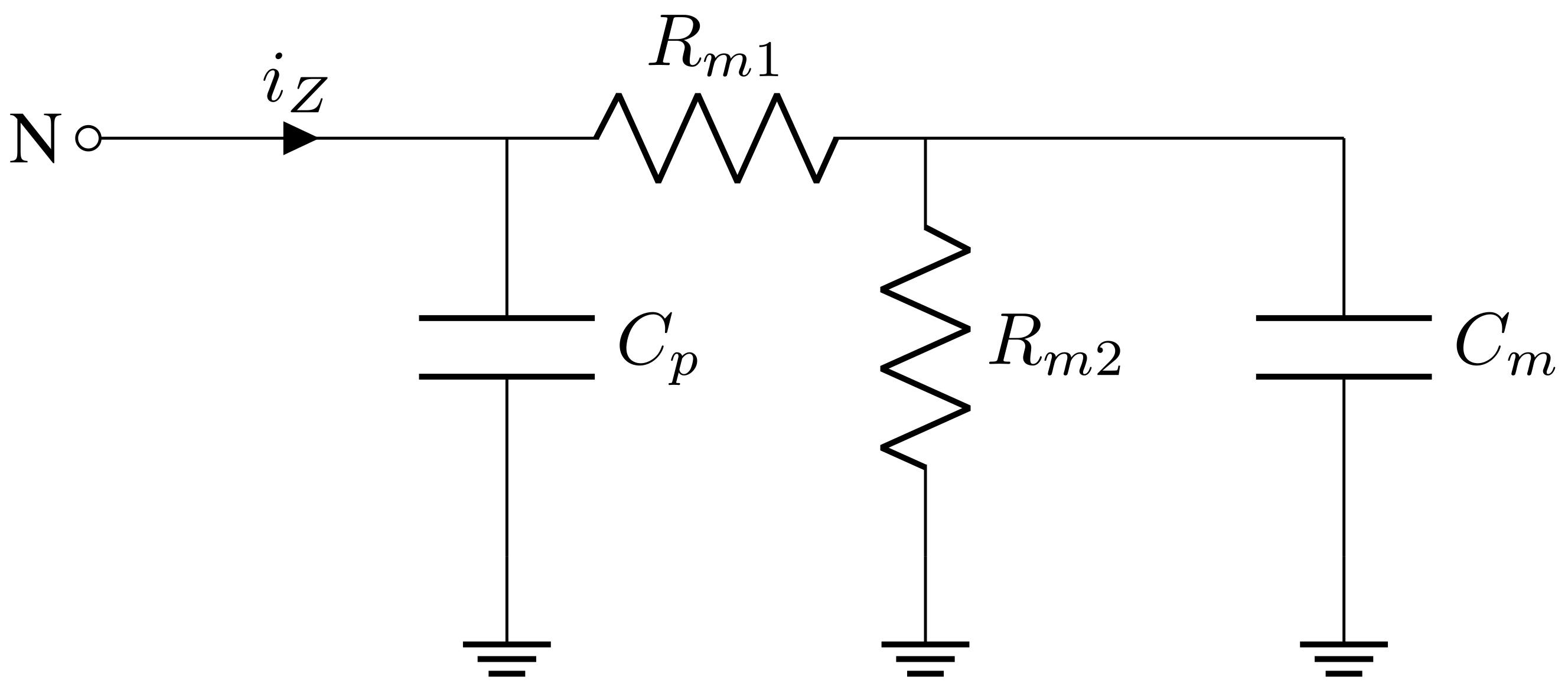
where $W_i\left(s\right)$ are strictly proper transfer functions with two poles and one zero and $e_i\left(s\right)$ and $p\left(s\right)$ are second-order polynomials in s. Let us now, instead, consider the case of an unbalanced three-phase machine where an impedance is connected between the star-point and ground. In particular, let us consider an impedance consisting of the parallel between a parasitic capacitance $C_p$ and a voltage divider with filtering action as shown in Figure 2, that is typically used for measuring the star-point voltage. Thus, the transfer function $Z\left(s\right)$ can be expressed as

$$Z\left(s\right)=\frac{A\left(1+s{\tau }_z\right)}{1+s{p}_1+s^2{p}_2},$$

(28)

where $A=\left(R_{m1}+R_{m2}\right)$, ${\tau }_z=\frac{R_{m1}{R}_{m2}{C}_m}{R_{m1}+R_{m2}}$, $p_1=R_{m2}{C}_m+C_p\left(R_{m1}+R_{m2}\right)$ and $p_2=R_{m1}{R}_{m2}{C}_m{C}_p$.

Figure 2. Schematic of a measuring impedance with a parallel parasitic capacitance.

Let us define the quantity $K=\frac{\left|{\mathbf{L}}_{abc}\right|}{A}$. Thus, the term $D\left(s\right)$ becomes the ratio of two polynomials in s and can be expressed as:

$$D\left(s\right)=\frac{sK\left|{\mathbf{Z}}_{abc}\right|\left(1+s{p}_1+s^2{p}_2\right)}{1+s{\tau }_z}+{\mathbf{L}}_{{\sum }_{abc}}\mathbf{M}\left(s\right){\mathbf{T}}^T=\frac{s\left[K\left|{\mathbf{Z}}_{abc}\right|\left(1+s{p}_1+s^2{p}_2\right)+\left(1+s{\tau }_z\right)p\left(s\right)\right]}{1+s{\tau }_z}.$$

(29)

By recalling the definition of the polynomials from (27), one can write the expression of the transfer functions $\mathbf{G}\left(s\right)$ as:

$$G_i\left(s\right)=\frac{e_i\left(s\right)\left(1+s{\tau }_z\right)}{K\left|{\mathbf{Z}}_{abc}\right|\left(1+s{p}_1+s^2{p}_2\right)+\left(1+s{\tau }_z\right)p\left(s\right)}=\frac{e_i\left(s\right)}{p\left(s\right)}\frac{f_i\left(s\right)}{t_i\left(s\right)},i=a,b,c,$$

(30)

where $f_i\left(s\right)$ and $t_i\left(s\right)$ are respectively polynomials of the first and third order in s:

$$\begin{array}{cc}\hfill f_i\left(s\right)& =1+s{\tau }_z,\hfill \\ \hfill t_i\left(s\right)& =\frac{K\left|{\mathbf{Z}}_{abc}\right|\left(1+s{p}_1+s^2{p}_2\right)}{p\left(s\right)}+\left(1+s{\tau }_z\right).\hfill \end{array}$$

(31)

It has to be remarked that, in general, the quantities K, $p_1$, $p_2$, and ${\tau }_z$ are relatively small compared to the time constants of the electrical equations of the machine. The terms $\frac{e_i\left(s\right)}{p\left(s\right)}$ model the dynamics of the electrical machine phases while $\frac{f_i\left(s\right)}{t_i\left(s\right)}$ model the impedance dynamics at the star-point voltage that is also dependent on the poles given by $p\left(s\right)$. The latter is characterized by a much faster dynamic than the former.

2.2. Extraction of the Position Information

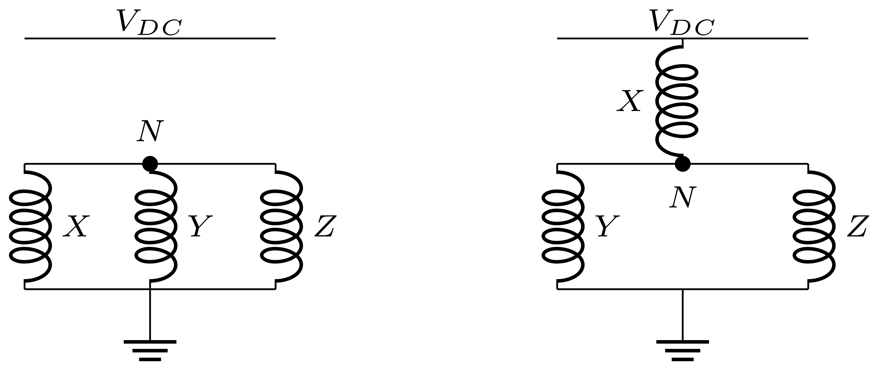
The quantities $L_{k_{{\sum }_i}}$ defined in (25) represent the ratio between the sum of the elements of the ith column of the adjoint matrix ${\mathbf{L}}_{abc}^{*}$ and the sum of all of its elements. Thus, given that the matrix ${\mathbf{L}}_{abc}$ is a function of the electrical angle ${\theta }_r$, it is possible to estimate the electrical angle of the machine by measuring the quantities $L_{k_{{\sum }_i}}$. Therefore, let us consider an SM driven by means of a three-phase inverter. Also, let us assume that no impedance is connected to the machine star-point. Let us define two excitation states of the machine as shown in Figure 3, where $X,Y,Z$ can be any distinct combination of phases $A,B,C$.

Figure 3. States of excitation 0 and I of permanent magnet synchronous motor (PMSM).

Let us now recall (18) where, for simplicity, zero initial conditions are considered:

$$V_{NO}=\mathbf{G}\left(s\right)\left({\mathbf{V}}_{XO}-{\omega }_r\mathbf{e}\frac{1}{s}\right),$$

(32)

where, recalling (27), one can express $\mathbf{G}\left(s\right)$ as

$$\mathbf{G}\left(s\right)=\left[\begin{array}{ccc}{L}_{k_{{\sum }_a}}+W_a\left(s\right)& L_{k_{{\sum }_b}}+W_b\left(s\right)& L_{k_{{\sum }_c}}+W_c\left(s\right)\end{array}\right]={\mathbf{L}}_{k_{\sum }}+\mathbf{W}\left(s\right).$$

(33)

Thus, the star-point voltage in the Laplace domain can be rewritten as

$$V_{NO}={\mathbf{L}}_{k_{\sum }}\left({\mathbf{V}}_{XO}-\frac{{\omega }_r\mathbf{e}}{s}\right)+\mathbf{W}\left(s\right)\left({\mathbf{V}}_{XO}-\frac{{\omega }_r\mathbf{e}}{s}\right).$$

(34)

Let us apply the Laplace antitransform that leads to:

$$v_{NO}\left(t\right)={\mathbf{L}}_{k_{\sum }}\left[{\mathbf{v}}_{XO}\left(t\right)-{\omega }_r\mathbf{e}1\left(t\right)\right]+\mathbf{w}\left(t\right)*{\mathbf{v}}_{XO}\left(t\right)-{\omega }_r\mathbf{w}\left(t\right)*\mathbf{e}1\left(t\right),$$

(35)

where $1\left(t\right)$ is the step function, $\mathbf{w}\left(t\right)={\mathcal{L}}^{-1}\left[\mathbf{W}\left(s\right)\right]$ and * is the convolution product operator. By defining the following time functions:

$$\begin{array}{c}\hfill b_A\left(t\right)=w_a\left(t\right)*v_{AO}\left(t\right),\\ \hfill b_B\left(t\right)=w_b\left(t\right)*v_{BO}\left(t\right),\\ \hfill b_C\left(t\right)=w_c\left(t\right)*v_{CO}\left(t\right),\end{array}$$

(36)

$$\begin{array}{c}\hfill c_A\left(t\right)=w_a\left(t\right)*e_{a}1\left(t\right),\\ \hfill c_B\left(t\right)=w_b\left(t\right)*e_{b}1\left(t\right),\\ \hfill c_C\left(t\right)=w_c\left(t\right)*e_{c}1\left(t\right),\end{array}$$

(37)

(35) can be rewritten as

$$v_{NO}\left(t\right)={\mathbf{L}}_{k_{\sum }}\left[{\mathbf{v}}_{XO}\left(t\right)-{\omega }_r\mathbf{e}1\left(t\right)\right]+\sum _{i=A,B,C}\left(b_i\left(t\right)-{\omega }_r{c}_i\left(t\right)\right).$$

(38)

Let us consider now the machine to be in the excitation state 0, where all machine phases are connected to ground, and that at a generic time $t_1>0$ a generic phase X, whose voltage is indicated as $v_{XO}\left(t\right)$, is switched to the inverter bus voltage $v_{DC}$. In the Laplace domain, we could define the terminal voltage $V_{XO}\left(s\right)$ as

$$V_{XO}\left(s\right)=\frac{v_{DC}}{s}{e}^{-t_{1}s},X\in \left\{A,B,C\right\}.$$

(39)

Thus, by applying the Laplace inverse transform to the terminal voltages we get that:

$$v_{XO}\left(t\right)=v_{DC}1(t-t_1),X\in \left\{A,B,C\right\},$$

(40)

$$v_{YO}\left(t\right)=0,\forall Y\in \left\{A,B,C\right\},Y\ne X.$$

(41)

Let us evaluate $v_{NO}\left(t\right)$ for $t\to t_1$ from the left ($t=t_1^{-}$) and from the right ($t=t_1^{+}$). One obtains

$$v_{NO}\left(t_1^{-}\right)=-{\mathbf{L}}_{k_{\sum }}{\omega }_r\mathbf{e}-{\omega }_r\sum _{i=A,B,C}{c}_i\left(t_1^{-}\right),$$

(42)

$$v_{NO}\left(t_1^{+}\right)=L_{k_{{\sum }_X}}{v}_{DC}-{\mathbf{L}}_{k_{\sum }}{\omega }_r\mathbf{e}+b_X\left(t_1^{+}\right)-{\omega }_r\sum _{i=A,B,C}{c}_i\left(t_1^{+}\right).$$

(43)

One can observe that $c_i\left(t_1^{-}\right)=c_i\left(t_1^{+}\right)$ for $i=A,B,C$. Also, ${\omega }_r$ and $\mathbf{e}$ are considered constant by hypothesis. Finally, one can prove that $b_X\left(t_1^{+}\right)=0$. In fact, for the initial value theorem one can write:

$$\underset{t\to t_1^{+}}{lim}{b}_X\left(t\right){{|}_{v_{XO}\left(t\right)=v_{DC}1(t-t_1)}=\underset{t\to 0}{lim}{b}_X\left(t\right)|}_{v_{XO}\left(t\right)=v_{DC}1\left(t\right)}=\underset{s\to \infty }{lim}s{W}_x\left(s\right)\frac{v_{DC}}{s}=0,$$

(44)

given that $W_x\left(s\right)$ is a strictly proper transfer function. So, the difference between the value of $v_{NO}$ when approaching $t=t_1$ from the right and from the left is

$$v_{NO}\left(t_1^{+}\right)-v_{NO}\left(t_1^{-}\right)=L_{k_{{\sum }_x}}{v}_{DC}.$$

(45)

To remove the common mode present among $L_{k_{{\sum }_x}}$, $L_{k_{{\sum }_y}}$, and $L_{k_{{\sum }_z}}$, it is preferable to measure the difference between the machine star-point voltage and an artificial star-point voltage $v_{VO}=\frac{1}{3}\mathbf{T}{\mathbf{v}}_{XO}$ obtained by connecting the terminal voltages to three resistors that are star-connected, as shown in Figure 4. The difference between these voltages is here referred to as $v_{NV}$. Thus, one can easily verify that:

$$v_{NV}\left(t_1^{+}\right)-v_{NV}\left(t_1^{-}\right)=\left(L_{k_{{\sum }_x}}-\frac{1}{3}\right)v_{DC}.$$

(46)

Figure 4. Virtual star-point.

Let us define the measurements vector:

$${\mathbf{\Gamma }}_{abc}=\left[\begin{array}{ccc}{\Gamma }_a& {\Gamma }_b& {\Gamma }_c\end{array}\right]=\left({\mathbf{L}}_{k_{\sum }}-\frac{1}{3}\mathbf{T}\right)v_{DC}.$$

(47)

To extract the position information, it is convenient to transform this vector into an orthogonal reference system such as $\alpha -\beta -\gamma$. Thus, one can obtain:

$${\mathbf{\Gamma }}_{\alpha \beta \gamma }={\mathbf{T}}_C{\mathbf{\Gamma }}_{abc}={\left[\begin{array}{ccc}{\Gamma }_{\alpha }& {\Gamma }_{\beta }& {\Gamma }_{\gamma }\end{array}\right]}^T,$$

(48)

where ${\mathbf{T}}_C$ is the Clarke transformation matrix. The reconstructed machine angle can be obtained by applying the arctangent function:

$${\widehat{\theta }}_r=arctan\left(\frac{{\Gamma }_{\beta }}{{\Gamma }_{\alpha }}\right).$$

(49)

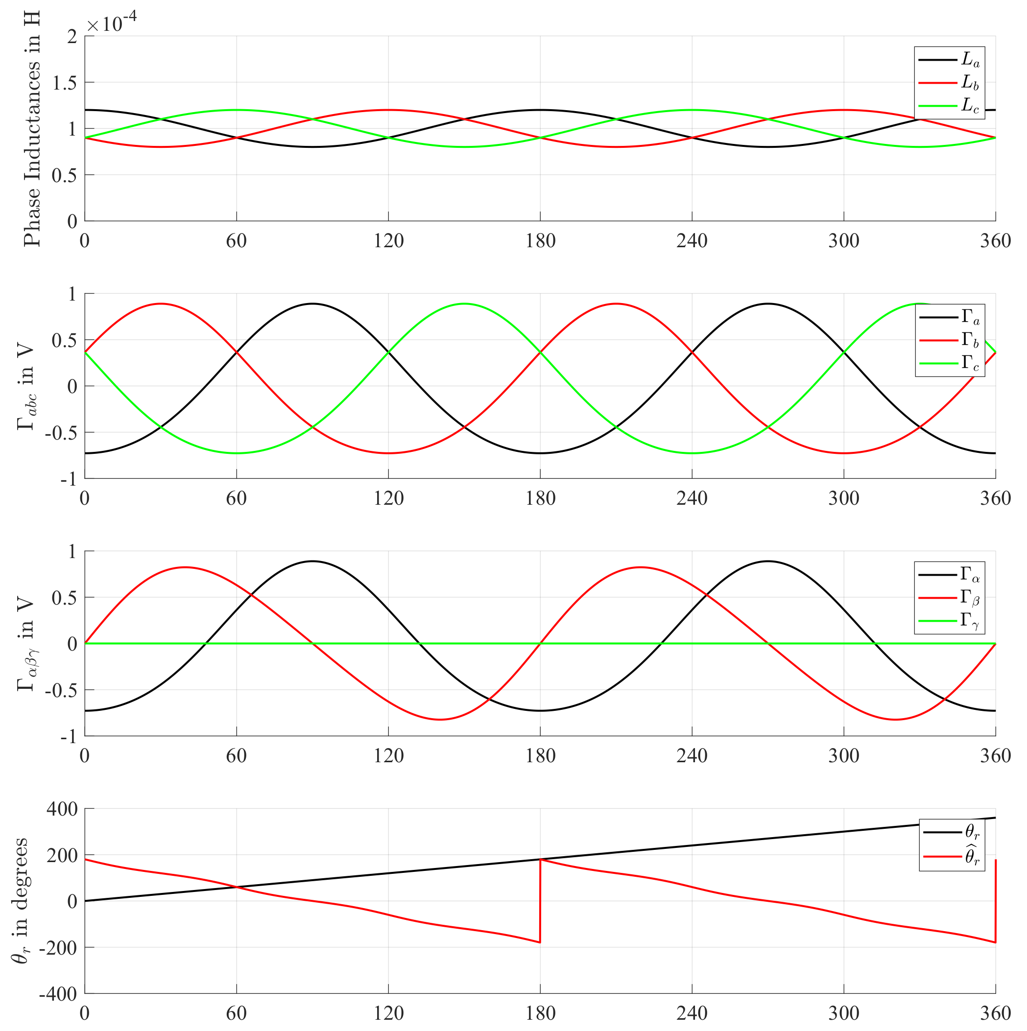
An example obtained in simulation is provided here. Let us consider a machine whose phase inductance matrix ${\mathbf{L}}_{abc}$ is defined as

$${\mathbf{L}}_{abc}=\left[\begin{array}{ccc}{L}_a& 0& 0\\ 0& L_b& 0\\ 0& 0& L_c\end{array}\right],$$

(50)

where $L_a=L_0+L_{2}cos\left(2\theta \right)$, $L_b=L_0+L_{2}cos\left(2\left(\theta +\frac{4}{3}\pi \right)\right)$, and $L_c=L_0+L_{2}cos\left(2\left(\theta -\frac{4}{3}\pi \right)\right)$ fluctuate in function of twice the rotor position. In this example, mutual inductances are ignored for simplicity. Nevertheless, this case corresponds to a class of tooth-wounded permanent magnet synchronous machines in certain combinations of poles and stator teeth, thus it refers to a real case. In Figure 5, the simulated self-inductances are shown with $L_0=100$ $\mathsf{\mu }$H and $L_2=20$ $\mathsf{\mu }$H. The ${\mathbf{\Gamma }}_{abc}$ and ${\mathbf{\Gamma }}_{\alpha \beta \gamma }$ are then shown in the case of an inverter bus voltage $v_{DC}=12$ V as well as the reconstructed rotor position ${\widehat{\theta }}_r$. It has to be remarked that the signals of ${\mathbf{\Gamma }}_{abc}$ and of ${\mathbf{\Gamma }}_{\alpha \beta \gamma }$ are not purely sinusoidal. In fact, such signals are obtained via the adjoint matrix of ${\mathbf{L}}_{abc}$, which is a matrix whose elements are obtained by multiplying the phase inductances. Thus, although the inductance matrix is made of purely sinusoidal terms representing a second harmonic with respect to the electrical angle, its adjoint matrix and, therefore, the signals in the vectors $\mathbf{\Gamma }$ present a fourth harmonic component, with different phase shifts in the $abc$ and $\alpha \beta \gamma$ frames. The reconstructed rotor position ${\widehat{\theta }}_r$ has a phase shift of $\pi$, moves in the opposite direction, and at twice the frequency of the rotor position. Nevertheless, compensation is trivial and further details concerning the extraction of the machine flux angle can be found in [17].

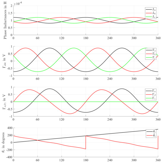
Figure 5. Simulated inductances, measurement vectors ${\mathbf{\Gamma }}_{abc}$, ${\mathbf{\Gamma }}_{\alpha \beta \gamma }$, and measured and estimated electrical rotor position.

3. Measurement of the ${\mathit{v}}_{\mathit{NV}}$ Voltage

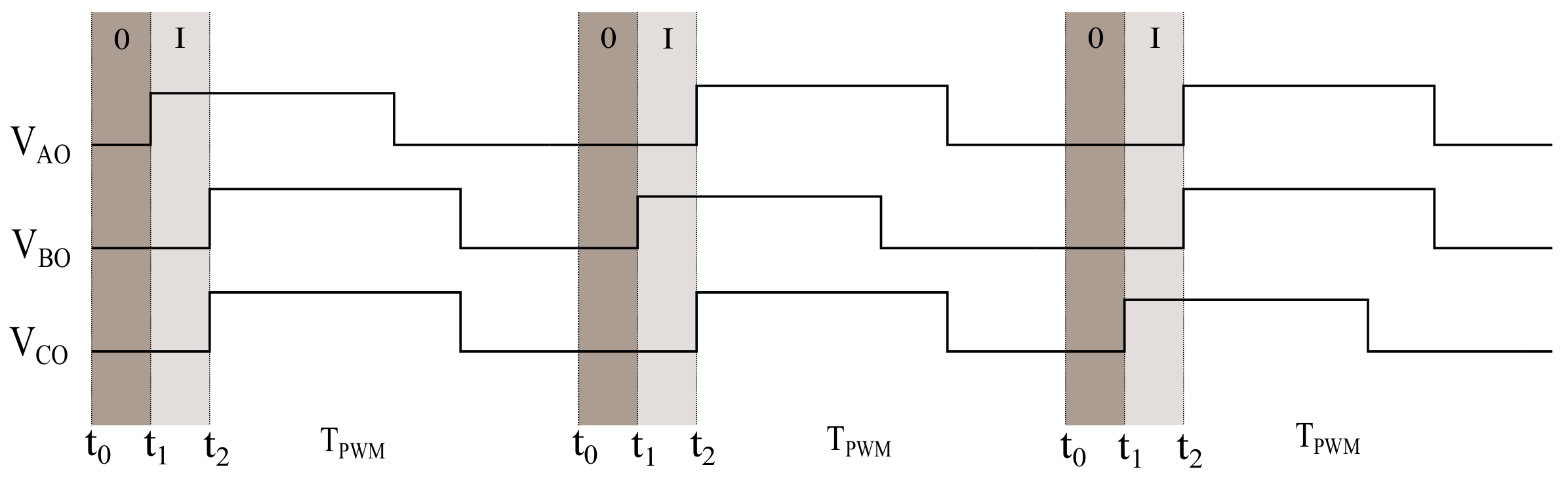
As discussed in the previous section, measuring the $v_{NV}$ voltage in the two excitation states of the machine shown in Figure 3 can retrieve the quantities ${\mathbf{\Gamma }}_{abc}$ that contain information about the machine phase inductances. For this reason, a modified edge-aligned PWM is proposed as shown in Figure 6, where the machine is driven in the excitation states 0 and I at the beginning of each PWM time period allowing measurements of the $v_{NV}$ voltage. In particular, the PWM time period starts at time $t_0$. One phase is then switched on at the time instant $t_1$ and, finally, the driving excitation according to standard edge-aligned PWM starts at the time instant $t_2$. During these two states of excitation, measurements can be performed. It is important to remark that the introduction in the PWM pattern of these two excitation states reduces the maximum applicable voltage to the machine. For this reason, it is of interest to reduce the time of injection of these two states.

Figure 6. Modified edge-aligned pulse width modulation (PWM) pattern used for measurement of the $v_{NV}$ voltage.

3.1. Direct Voltage Measurement

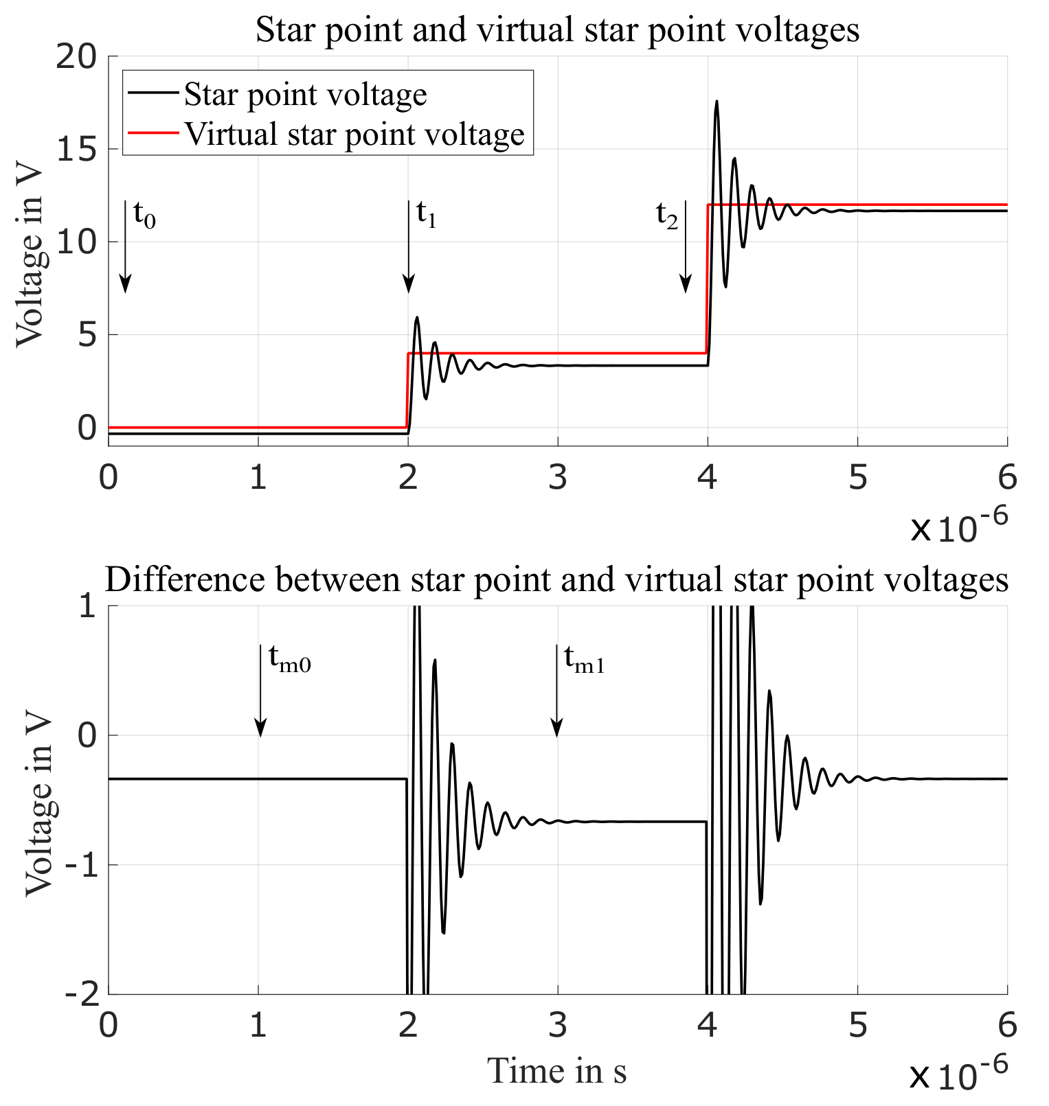
To measure ${\mathbf{\Gamma }}_{abc}$, a straightforward method is to measure the voltage $v_{NV}$ right before and after the switching between the machine excitations 0 and I. In this work, this measurement method is referred to as direct voltage measurement (DVM). Figure 7 shows the simulated response of $v_{NO}$, $v_{VO}$, and $v_{NV}$. As one can see, voltage oscillations are present, as described previously, due to the measuring impedance as well as to the parasitic capacitance. Measurements are performed at the generic time instants $t_0<t_{m0}<t_1$ and $t_1<t_{m1}<t_2$, providing $v_{NV}\left(t_{m0}\right)$ and $v_{NV}\left(t_{m1}\right)$. Ideally, it is preferable to choose $t_{m0}\to t_1^{-}$ and $t_{m1}\to t_1^{+}$. Nevertheless, especially concerning the measurements performed at $t_{m1}$, it is important to wait for the oscillations to decay to reduce measurement disturbances. Also, oscillations depend strictly on the machine parameters as well as on the impedance connected at the star-point, thus leading in some cases to a significant time for the oscillations to decay and, therefore, reducing the maximum applicable voltage.

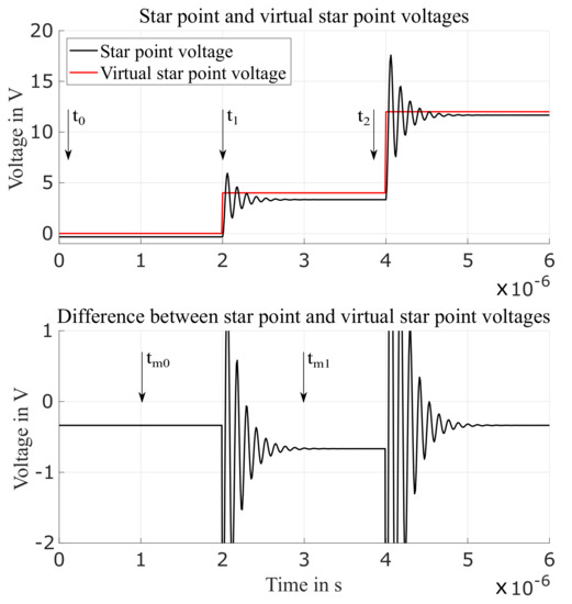
Figure 7. Simulated response of the star-point voltages at the machine excitation states 0 and I.

3.2. Fast Resettable Integrator Circuit

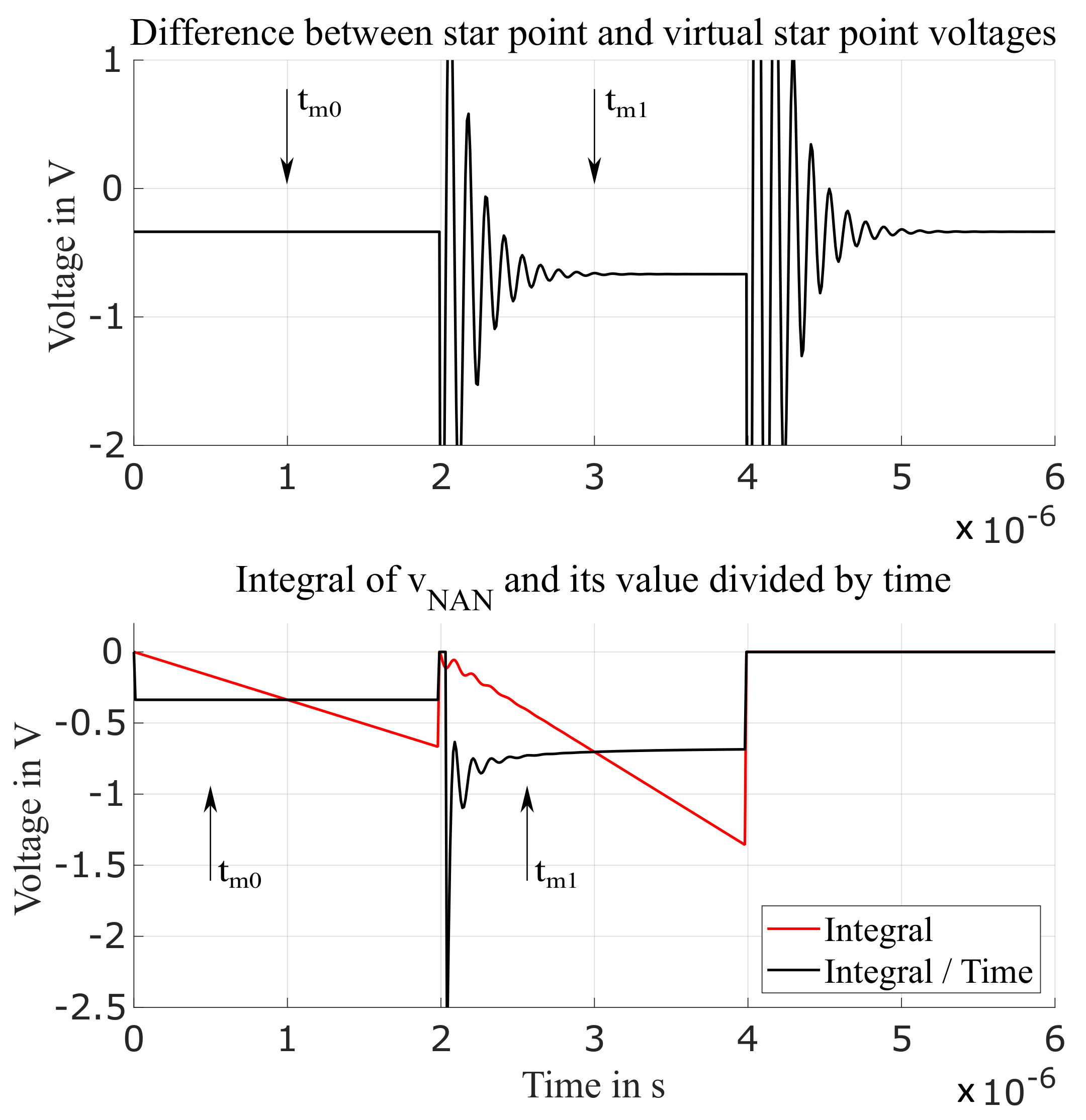
Another method to measure ${\mathbf{\Gamma }}_{abc}$ is the usage of a fast resettable integrator circuit (FRIC). This technique is based on measuring the integral of the $v_{NV}$ voltage. An analog integrator connected to the machine star-point and to the virtual star-point is activated when the machine state of excitation 0 is injected, thus integrating the voltage $v_{NV}$ during the time of the machine excitation. The integrator is then reset before the machine state of excitation I is provided. At the end of the application of this excitation state, the integrator is held in reset until the next PWM period. Figure 8 shows the integration applied to the $v_{NV}$ voltage already presented in Figure 7. As one can see, the oscillation affecting the integrated voltage decays much faster than in the case of DVM, thus allowing a measurement to be performed earlier and, consequently, to reduce the injection time of the excitation necessary to obtain the ${\mathbf{\Gamma }}_{abc}$ quantities thus increasing the maximum applicable voltage. Let us define the quantities $I_0$ and $I_1$ as the measurements of the integral of $v_{NV}$ at the time instants $t_{m0}$ and $t_{m1}$, respectively. Let us also define the time intervals $\Delta t_0=t_{m0}-t_0$ and $\Delta t_1=t_{m1}-t_1$. To obtain the quantities of interest, one can use the following equations:

$$\begin{array}{cc}\hfill & v_{NV}\left(t_{m0}\right)\approx \frac{I_0}{\Delta t_0},\hfill \\ \hfill & v_{NV}\left(t_{m1}\right)\approx \frac{I_1}{\Delta t_1}.\hfill \end{array}$$

(51)

Figure 8. Simulated integration of the $v_{NV}$ voltage and the corresponding measurement.

The obtained measurements only approximate to the real value of $v_{NV}$ due to the presence of oscillations. Nevertheless, it has to be remarked that $v_{NV}\left(t_{m0}\right)$ resembles closely the real value. In fact, during the state of excitation, 0 oscillations have usually already decayed at the beginning of a PWM time period. Concerning $v_{NV}\left(t_{m1}\right)$, one can observe that the obtained value is proportional to the reference value, thus introducing a small deviation from the measurements performed by means of DVM. Proposing a mathematical description of such deviation is particularly challenging, nevertheless it can be observed numerically that the proportionality factor between the FRIC measurements and the reference values do not change as long as $\Delta t_1$, the oscillation frequency, and the damping factor do not change. Thus, it is possible to conclude that measurements obtained by means of the FRIC resemble closely the measurements obtained by DVM, while allowing a reduction of the needed time of the injection of the necessary excitation for measuring ${\mathbf{\Gamma }}_{abc}$ and, therefore, an increase of maximum applicable voltage. In both the discussed approaches, the measurement circuitry needs to be turned on the specific machine to obtain optimal measurements.

3.3. Measurement Electronics

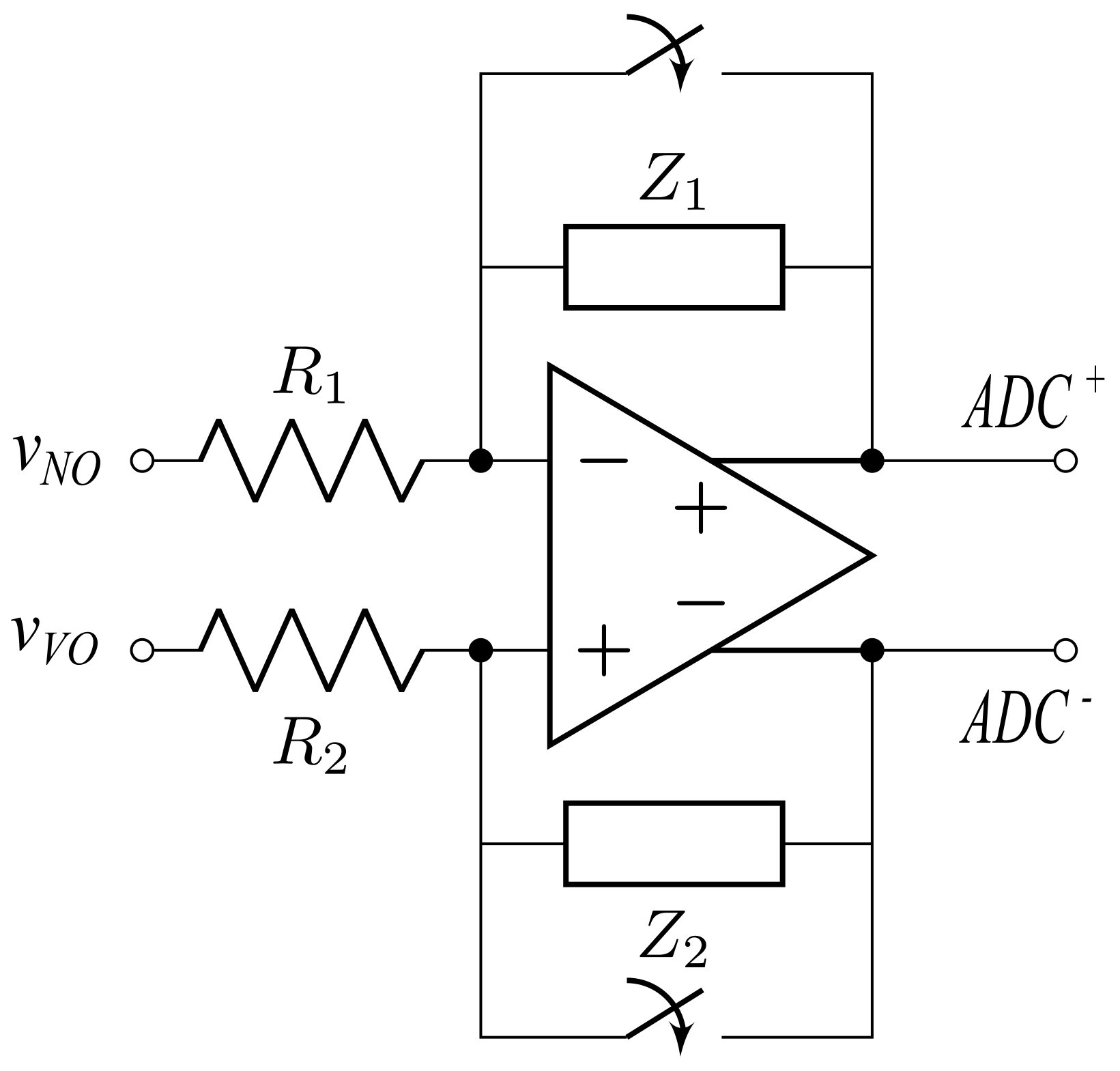
Measuring $v_{NV}$ requires dedicated electronics. In Figure 9, an electronic schematic is proposed that can either be used for DVM or for FRIC, which is based on a differential operational amplifier and its output is a differential voltage. For DVM operation, the impedances Z are resistors. Also, the reset mechanism is not used. In particular, given $Z_1=Z_2=R_f$ and $R_1=R_2=R$, this stage has a gain equal to $\frac{R_f}{R}$. Such gain needs to be adjusted to provide a reliable measurement without bringing the measurement stage into saturation. When operating as a FRIC, the impedances $Z_1$ and $Z_2$ are capacitors. In this case, the stage is tuned by setting $Z_1=Z_2=\frac{1}{s{C}_f}$ and by considering that the gain of the integrator stage is given by $\frac{1}{R{C}_f}$, where $R_1=R_2=R$. In this case, the gain also needs to be adjusted to provide a measurement that does not drive the measuring stage into saturation. Moreover, the reset mechanism is used to mantain the integrator in reset when no measurement is performed. In this case, the feedback capacitors $C_f$ are shortcircuited and the output is zero.

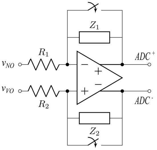
Figure 9. Schematic of the measuring electronics.

4. Experimental Validation

To evaluate the different performance between the DVM and the FRIC approaches, an experimental test-bench has been set up. A PMSM has been used as a test device whose electrical parameters are listed in Table 1.

Table 1. List of parameters of the PMSM used for experimental validation.

Parameter	Value
Phase resistance	2.2 $\Omega$
$L_d$ inductance	394 $\mathsf{\mu }$H
$L_q$ inductance	475 $\mathsf{\mu }$H
Back-EMF constant	118.6 mVs
Number of pole pairs	8
Nominal voltage	24 V

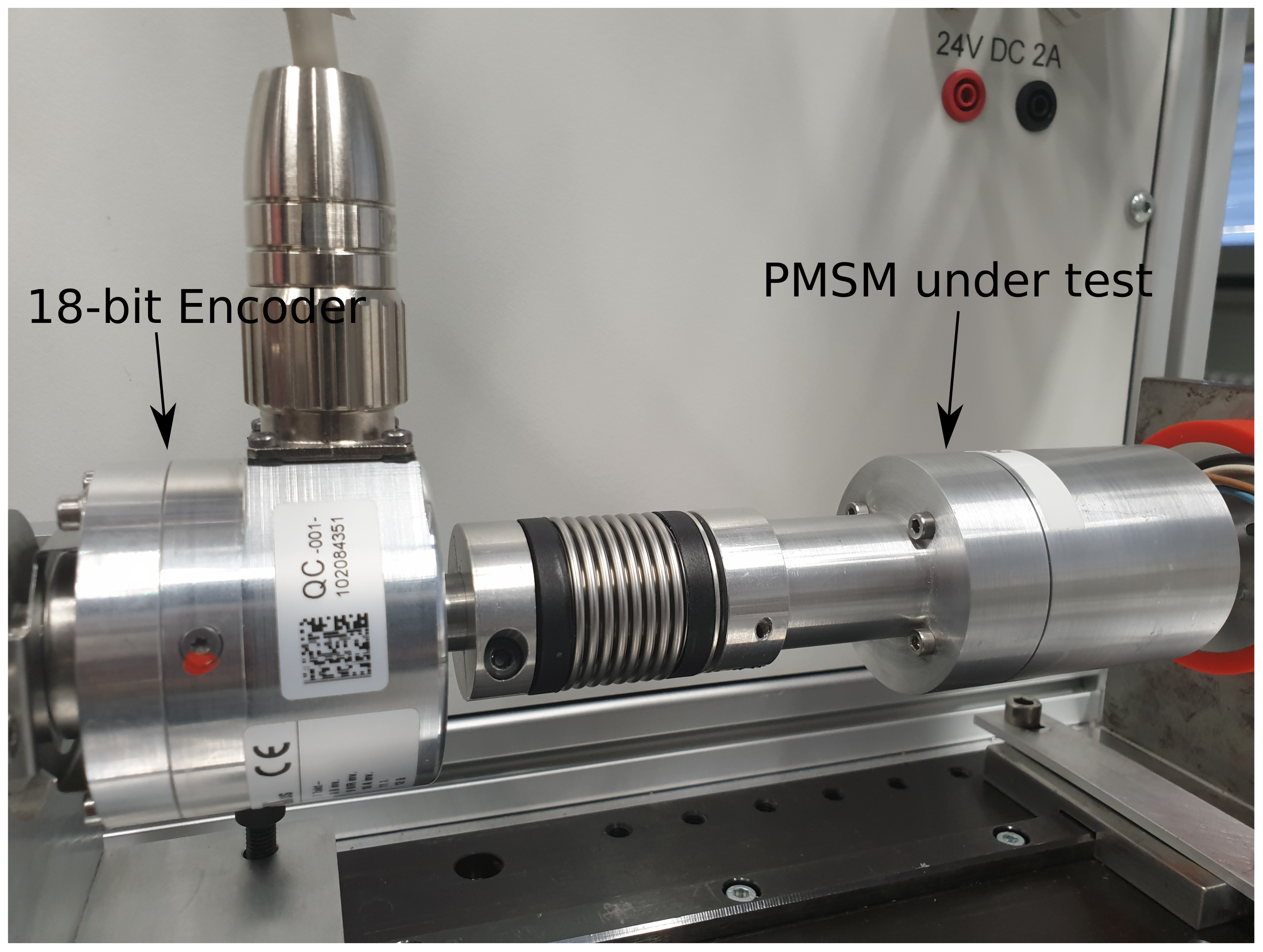
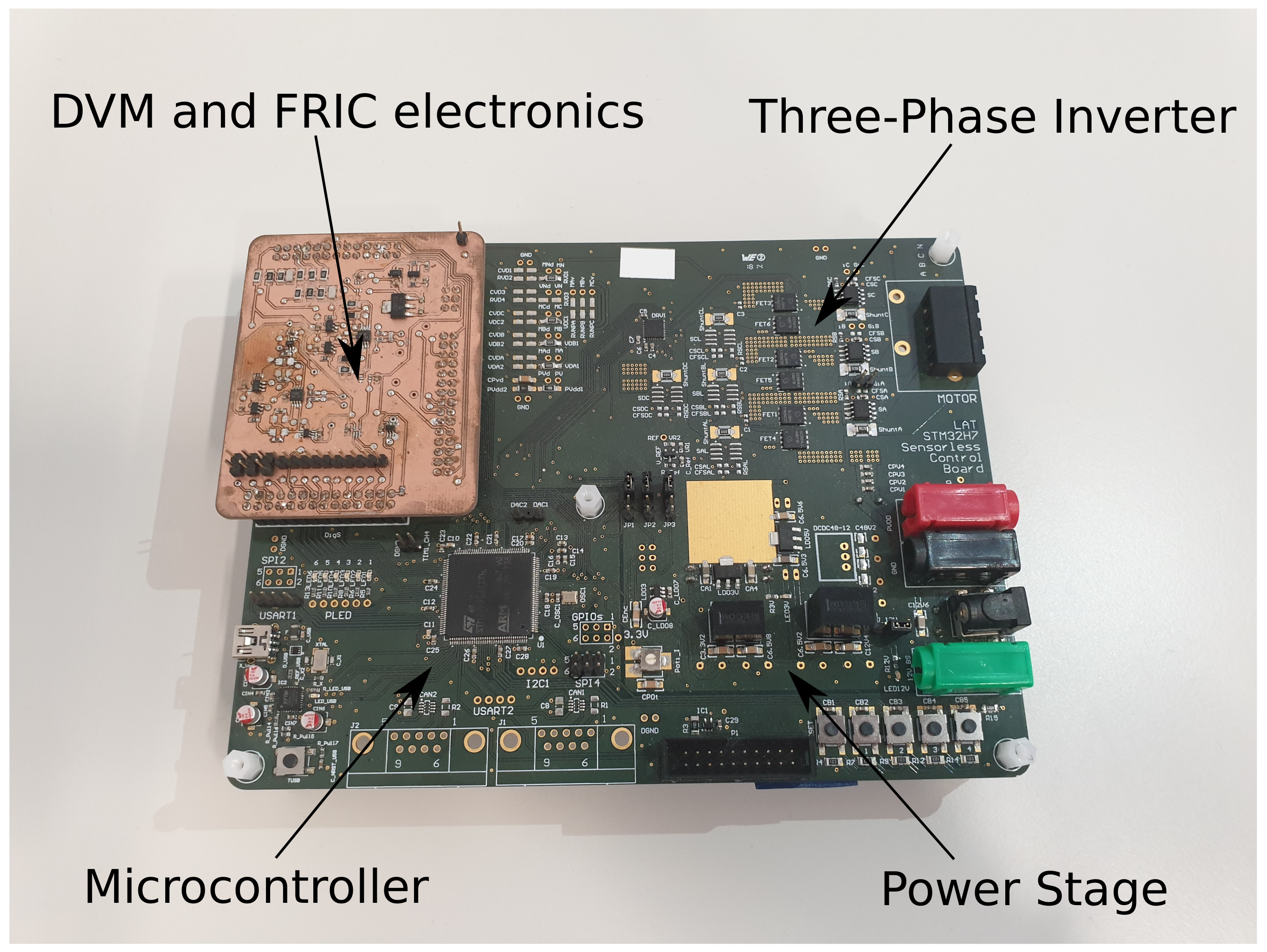
The PMSM has been coupled to a Baumer GBA2H 18 bit encoder and to a servomotor. An electronic board based on a 32-bit microcontroller, a three-phase MOSFET-based inverter, and dedicated electronics for implementing both the DVM and FRIC has been developed. The chosen microcontroller features 16-bit ADCs and a clock frequency of 400 MHz, which allows high timing precision in generating the required reset and sampling triggers of the FRIC circuitry. A dedicated USB based communication protocol is implemented to measure and record the obtained signals at high frequency. Figure 10 and Figure 11 show the experimental bench and the electronic board, respectively.

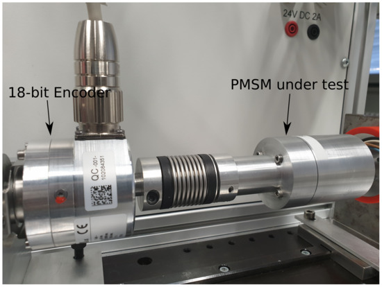
Figure 10. The PMSM under test coupled to a 18-bit encoder.

Figure 11. The microcontroller-based electronics used for experimental validation.

The electronic circuit implementing DVM is based on the schematic shown in Figure 9 where $R_1=R_2=1$ k$\Omega$ and $Z_1=Z_2=10$ k$\Omega$, allowing an amplification of the $v_{NV}$ voltage equal to 10. The FRIC electronics, instead, has been tuned by setting $R_1=R_2=120$ $\Omega$ and $Z_1=Z_2$ are capacitors whose value is 470 pF. The choice of these parameters corresponds to an integration time constant equal to $56.4$ ns. For both circuitries, a high-bandwidth differential operational amplifier has been chosen. The differential voltage $v_{NV}$ is scaled by means of voltage dividers and provided to the measurement circuit through a stage of voltage buffering. Both circuits operate in parallel to allow a comparison of performance between DVM and FRIC during the same experiment.

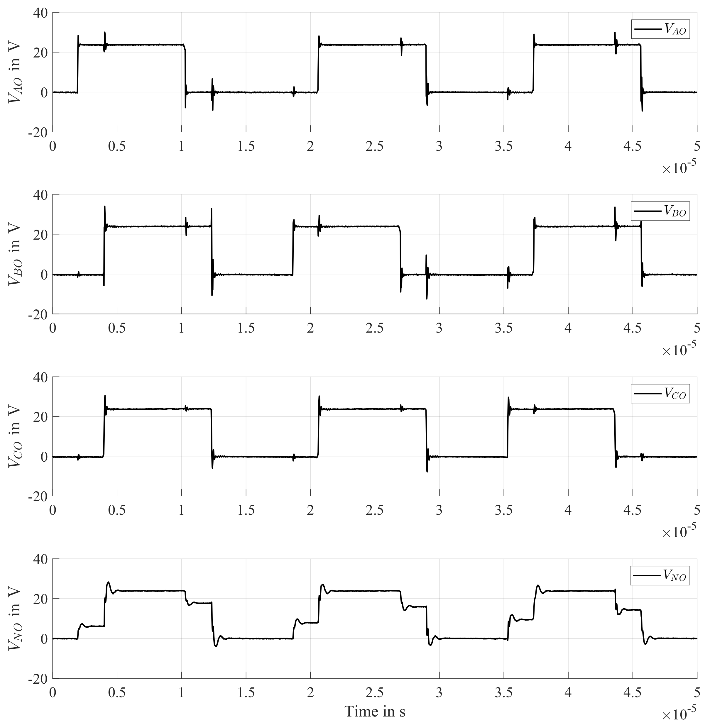
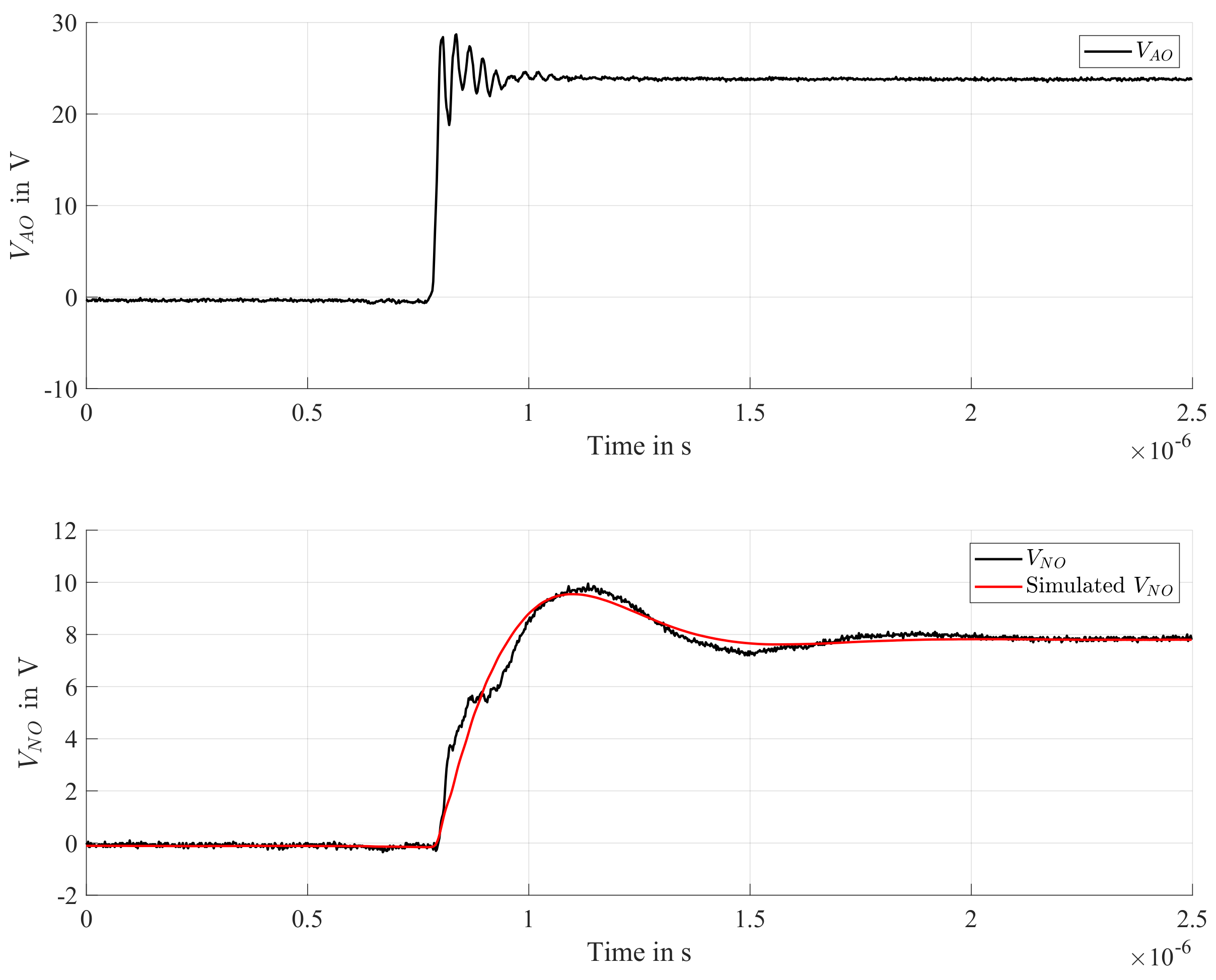
The three-phase inverter operates at a bus voltage of 24 V and is driven by means of the modified edge-aligned PWM pattern described earlier and shown in Figure 6. In Figure 12, the measured phase voltages ${\mathbf{v}}_{XO}$ and $v_{NO}$ are shown. In this case, a duty cycle of 50% has been applied to all phases. To verify (30), the $v_{NO}$ voltage has been measured during the transition of the machine from the excitation state 0 to the excitation state I, by switching the phase voltage $v_{AO}$ to the inverter bus voltage and leaving $v_{BO}$ and $v_{CO}$ connected to ground. In fact, as shown previously, the transfer functions in (30) can be expressed as the series of an ideal transfer function representing the machine electrical behavior and a high-frequency transfer function modeling the presence of an impedance connected to the machine star-point, especially for the case of a parasitic capacitance in addition to a measuring circuit that, in this case, is given by the oscilloscope probe used for measuring $v_{NO}$. A linear transfer function with 3 poles and 1 zero (as predicted by the mathematical derivation proposed earlier) has been identified by means of a nonlinear least-squares algorithm to approximate the star-point voltage response. This procedure has retrieved an adherence between the measured and the simulated responses of 93.84%, and results are shown in Figure 13, where the voltages $v_{AO}$, $v_{NO}$, and the output of the simulated model are shown. It has to be remarked that the proposed mathematical model does not take into account the presence of eddy currents.

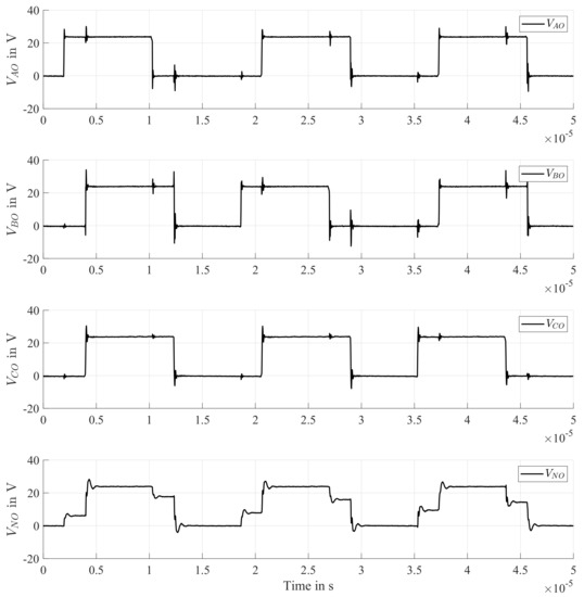
Figure 12. Applied PWM pattern and measured $v_{NO}$ voltage.

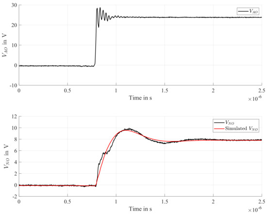
Figure 13. High-frequency dynamics of the $v_{NO}$ voltage modeled with a linear transfer function having three poles and one zero.

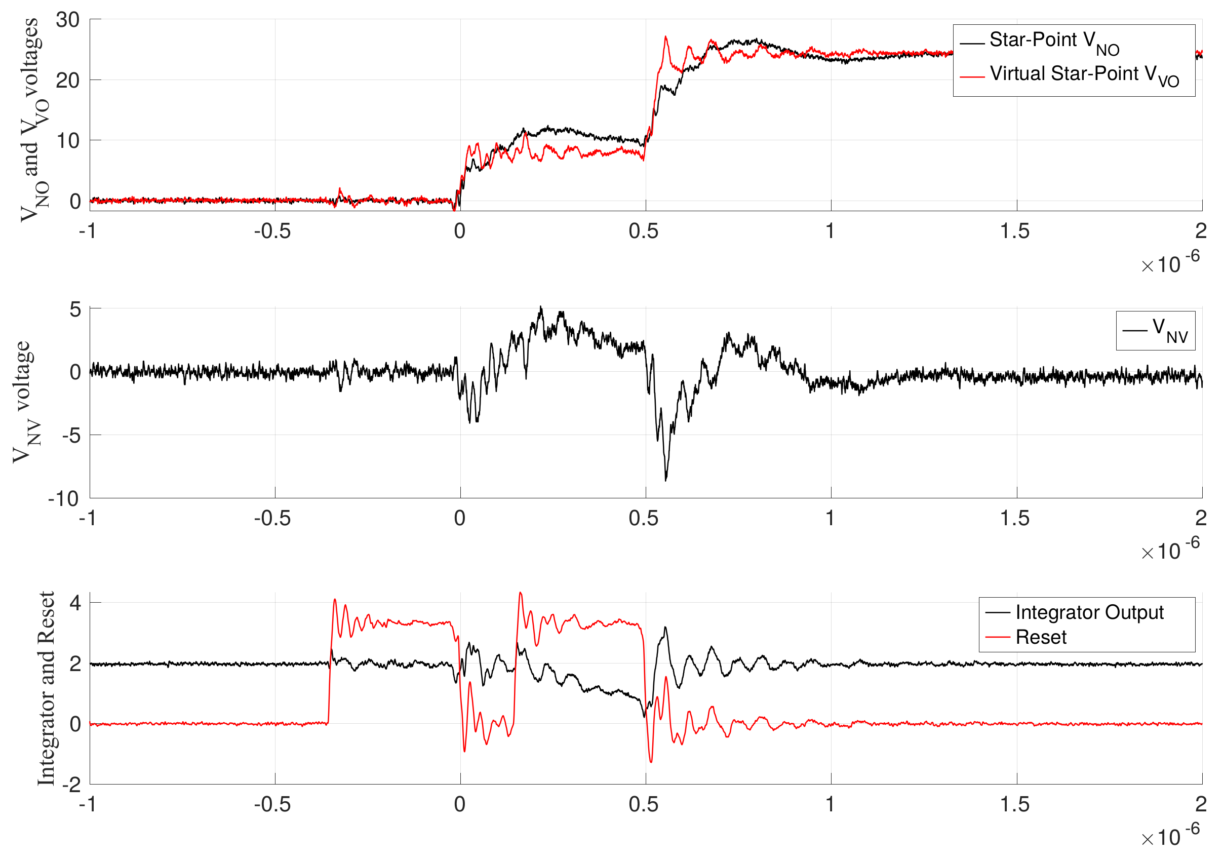
Measurements of the resulting $v_{NO}$, $v_{VO}$, and $v_{NV}$ voltages are shown in Figure 14, where the FRIC output and the reset trigger are shown for completeness. The FRIC is enabled when the reset voltage is at a high level, i.e., $3.3$ V.

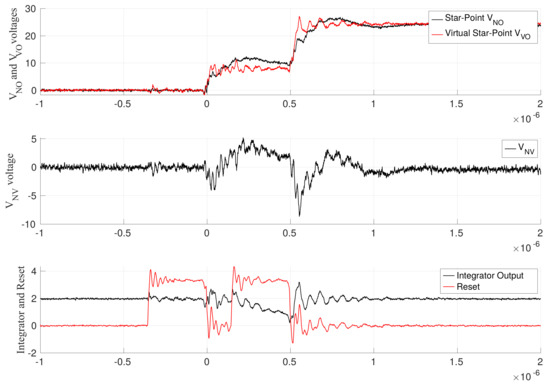
Figure 14. $v_{NV}$ voltages generated by the modified edge-aligned PWM pattern, with fast resettable integrator circuit (FRIC) output and reset trigger voltage.

The chosen PWM frequency is 60 kHz, corresponding to a PWM time period of $16.6$ $\mathsf{\mu }$s while the time delay for measurements is of 1 $\mathsf{\mu }$s. Thus, the maximum applicable driving voltage decreases by 6%. For this reason, it is generally preferable to keep the measurement time delay as small as possible to maximize the PMSM driving capability. The PMSM remains in the excitation state 0 from time $-0.5$ $\mathsf{\mu }$s to 0 s and in the excitation state I from 0 s to $0.5$ $\mathsf{\mu }$s. In the case of DVM, measurements are acquired at times $t_{m0}=-0.2$ $\mathsf{\mu }$s and $t_{m1}=0.3$ $\mathsf{\mu }$s. The FRIC circuitry, instead, is enabled for a time period of 300 ns during both excitation states, as shown in Figure 14, and measurements are triggered at the same time instants used for DVM.

Experimental Results

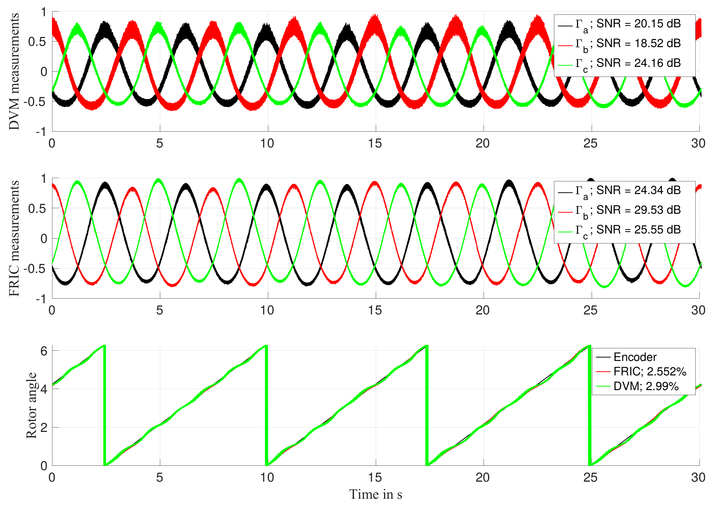
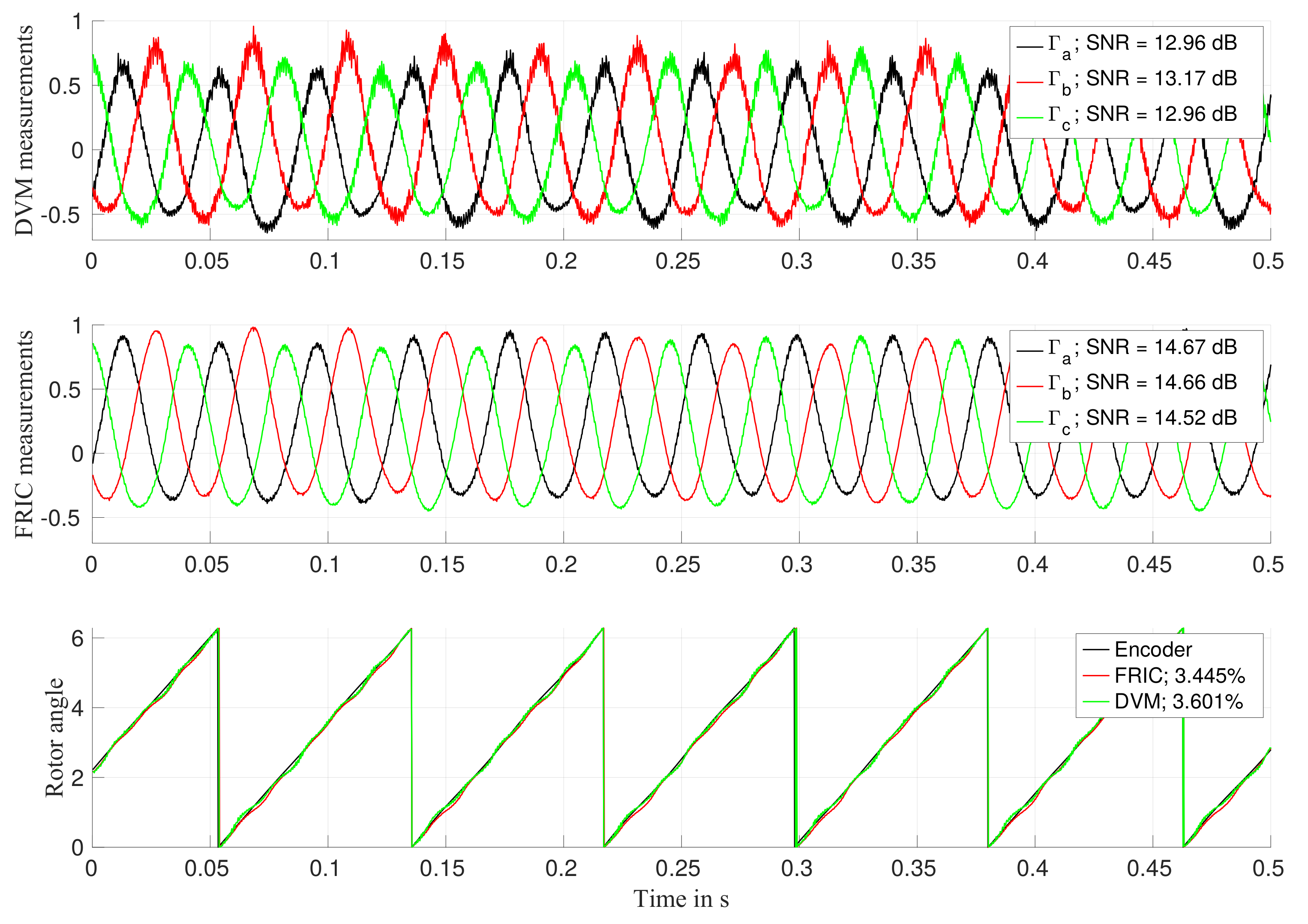
Experimental investigations have been conducted under two scenarios. Firstly, the PMSM has been coupled to a servomotor that is used to impose a rotation of 1 revolution per minute (RPM) to the PMSM to measure ${\mathbf{\Gamma }}_{abc}$ by means of DVM and FRIC in almost standstill conditions. The PMSM has been driven at zero current condition by driving all phases at $50\%$ duty cycle. Figure 15 shows the obtained results, where the ${\mathbf{\Gamma }}_{abc}$ signals have been normalized.

Figure 15. ${\mathbf{\Gamma }}_{abc}$ and reconstructed position with applied rotation at 1 revolutions per minute (RPM) by means of direct voltage measurement (DVM) and FRIC.

The signal-to-noise ratio (SNR) has been evaluated per each measured signal. Given that ${\mathbf{\Gamma }}_{abc}$ is composed of non purely sinusoidal signals, the SNR has been evaluated by calculating the fundamental frequency and by considering all harmonics beyond the 5th one as noise. As one can see, the measured ${\mathbf{\Gamma }}_{abc}$ exhibits higher SNR when the FRIC approach is used. The reconstructed position is then compared to the position given by the encoder. In this case, the percentage error has been evaluated. In this case, FRIC has provided a maximum position error of $2.55\%$ while DVM provides a maximum position error of $2.99\%$. One can also observe that the signals ${\mathbf{\Gamma }}_{abc}$ obtained by applying DVM or FRIC are similar but not equal as the FRIC method introduces a deviation from the reference value as discussed earlier.

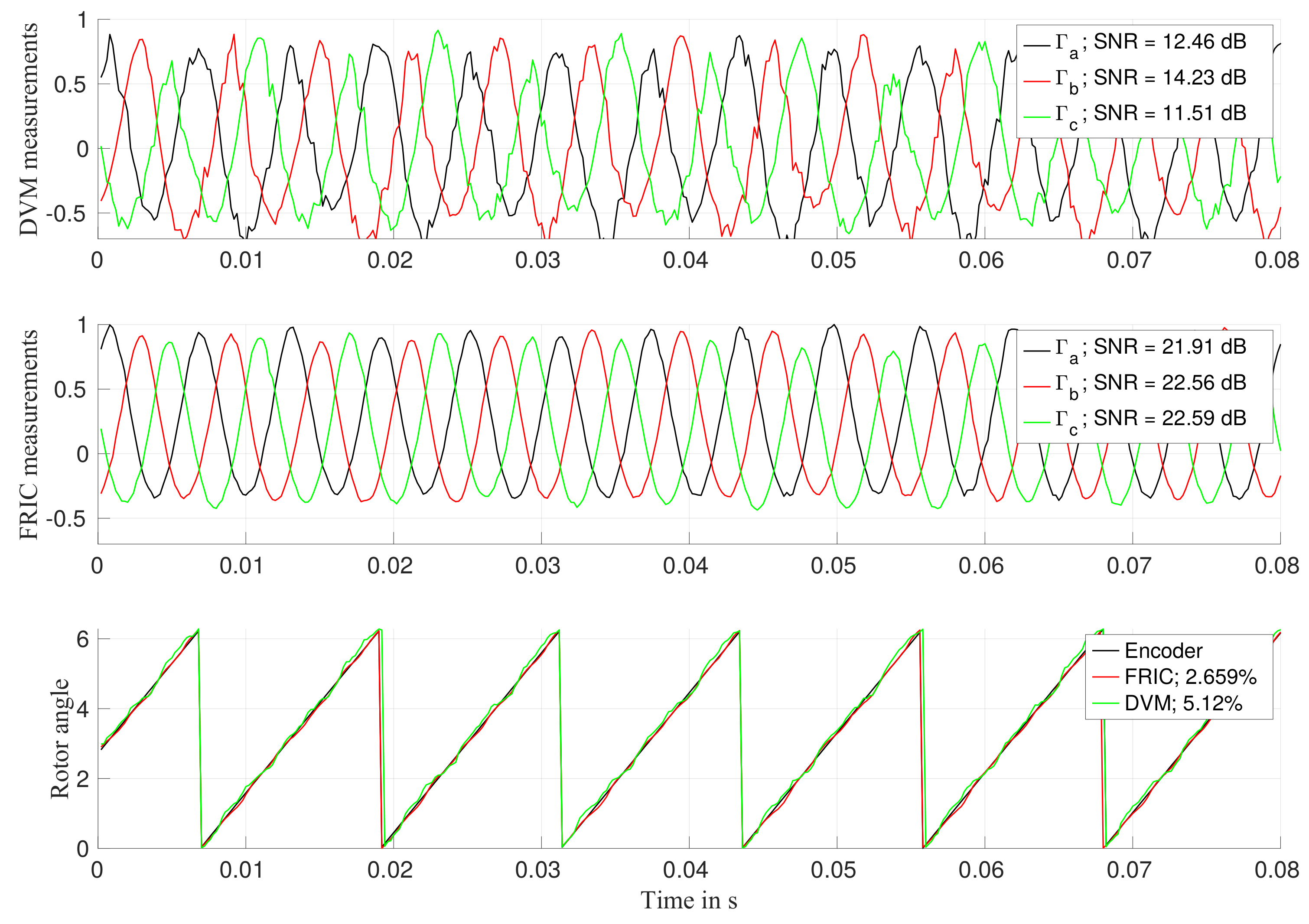
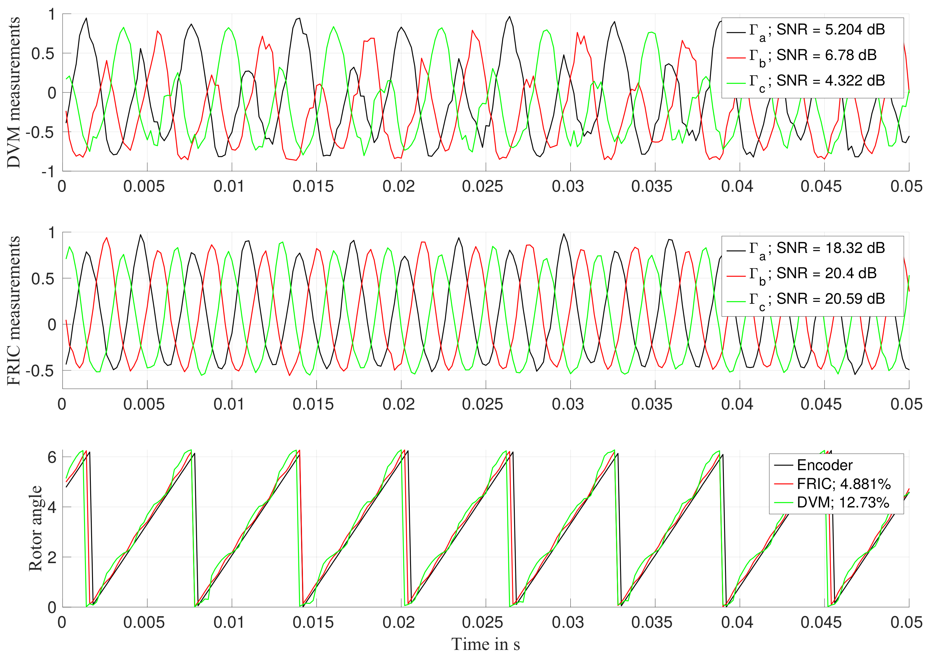
Afterward, a comparison between DVM and FRIC has been conducted by driving the machine under no-load driving conditions in order to evaluate performances at higher speeds. Also, the rotor angle obtained by means of the FRIC approach has been used for driving the machine. Figure 16, Figure 17 and Figure 18 show the measured ${\mathbf{\Gamma }}_{abc}$ and reconstructed electrical positions when driving the PMSM with 1 V, 6 V and 12 V along the q-axis, respectively. In these cases, the PMSM under test rotates at respective speeds of 91.3 RPM, 614.5 RPM, and 1199.7 RPM. In all these measurements, the evaluated SNR is higher when the FRIC circuit is used, especially when the maximum voltage is applied. In this case, the measured ${\mathbf{\Gamma }}_{abc}$ begins to distort, as visible in Figure 18. More important is the electrical position error obtained by using the DVM and the FRIC approaches. In fact, in the first case, the position error ranges from $3.6\%$ at 1 V to $12.73\%$ at the maximum voltage. In the case of FRIC, instead, the position error ranges from $3.4\%$ at 1 V to $4.88\%$ at the maximum voltage.

Figure 16. ${\mathbf{\Gamma }}_{abc}$ and reconstructed position by driving a q-axis voltage of 1 V.

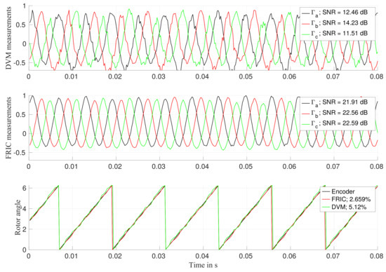
Figure 17. ${\mathbf{\Gamma }}_{abc}$ and reconstructed position by driving a q-axis voltage of 6 V.

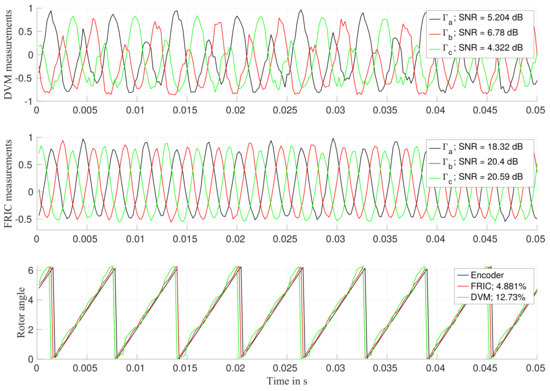
Figure 18. ${\mathbf{\Gamma }}_{abc}$ and reconstructed position by driving a q-axis voltage of 12 V.

5. Conclusions and Future Works

In this work, a new mathematical description of the star-point voltage dynamics has been proposed by considering also the presence of a measurement impedance and a parasitic capacitance. It has been observed that the transfer functions between the star-point voltage and the terminal voltages are proper second-order transfer functions whose static gains are given by the quantities $L_{k_{{\sum }_i}}$ that depend directly on the adjoint matrix of the machine inductance matrix ${\mathbf{L}}_{abc}$. Differently from previous works, the proposed mathematical description does not consider a particular form of the inductance matrix with the only condition being the inductance matrix to be non-singular. Two different approaches have been proposed to measure the differential voltage between the star-point and the artificial star-point, namely DVM and FRIC. Conducted experiments have shown the capability of the FRIC to provide, in general, less noisy measurements than DVM and, also, a smaller position error. Nevertheless, it has to be remarked that nonlinear effects, such as the influence of the eddy currents and power-stage ringing, have been neglected. Therefore, future works will be conducted to improve the proposed mathematical model as well as the measurement circuitry. Concerning the measurement technique, the choice of the trigger time instants is made preliminarily on the device under test. A more rigorous approach in tuning the measurement circuits and time instants is to be researched. Moreover, it will be of interest to particularize the presented mathematical framework for some specific machine typologies, such as permanent magnet synchronous motors and synchronous reluctance machines. In fact, the dependency of the machine phase inductances on the rotor position may differ drastically, in particular due to the behavior of the mutual inductances that, as seen in this paper, contribute to the information extractable from the star-point. For this reason, a deeper investigation on the influence of the mutual inductances on the reconstructed electrical angle is currently under investigation.

6. Patents

The FRIC circuit has been submitted for patenting and reference can be found in [18].

References

- Schrödl, M. Sensorless Control of A. C. Machines; Fortschritt-Berichte VDI: Reihe 21, Elektrotechnik 117; VDI-Verl: Düsseldorf, Germany, 1992; Volume 117. [Google Scholar]
- Schrödl, M. Sensorless control of AC machines at low speed and standstill based on the “INFORM” method. In Proceedings of the IAS ’96—Conference Record of the 1996 IEEE Industry Applications Conference Thirty-First IAS Annual Meeting, San Diego, CA, USA, 6–10 October 1996; Volume 1, pp. 270–277. [Google Scholar] [CrossRef]
- Lorenz, R.D. Transducerless Position and Velocitv Estimation in Induction and Salient AC Machines. IEEE Trans. Ind. Appl. 1995, 31, 240–247. [Google Scholar]
- Corley, M.; Lorenz, R. Rotor position and velocity estimation for a salient-pole permanent magnet synchronous machine at standstill and high speeds. IEEE Trans. Ind. Appl. 1998, 34, 784–789. [Google Scholar] [CrossRef]
- Linke, M.; Kennel, R.; Holtz, J. Sensorless position control of permanent magnet synchronous machines without limitation at zero speed. In Proceedings of the IEEE 2002 28th Annual Conference of the Industrial Electronics Society (IECON 02), Sevilla, Spain, 5–8 November 2002; Volume 1, pp. 674–679. [Google Scholar] [CrossRef]
- Linke, M.; Kennel, R.; Holtz, J. Sensorless speed and position control of synchronous machines using alternating carrier injection. In Proceedings of the IEEE International Electric Machines and Drives Conference (IEMDC’03), Madison, WI, USA, 1–4 June 2003; Volume 2, pp. 1211–1217. [Google Scholar] [CrossRef]
- Landsmann, P.; Paulus, D.; Stolze, P.; Kennel, R. Saliency based encoderless predictive torque control without signal injection. In Proceedings of the IEEE 2010 International Power Electronics Conference (ECCE ASIA), Sapporo, Japan, 21–24 June 2010; pp. 3029–3034. [Google Scholar] [CrossRef]
- Paulus, D.; Landsmann, P.; Kennel, R. Sensorless field- oriented control for permanent magnet synchronous machines with an arbitrary injection scheme and direct angle calculation. In Proceedings of the IEEE 2011 Symposium on Sensorless Control for Electrical Drives, Birmingham, UK, 1–2 September 2011; pp. 41–46. [Google Scholar] [CrossRef]
- Paulus, D.; Landsmann, P.; Kennel, R. Saliency based sensorless field- oriented control for permanent magnet synchronous machines in the whole speed range. In Proceedings of the 3rd IEEE International Symposium on Sensorless Control for Electrical Drives (SLED 2012), Milwaukee, WI, USA, 21–22 September 2012; pp. 1–6. [Google Scholar] [CrossRef]
- Friedmann, J.; Hoffmann, R.; Kennel, R. A new approach for a complete and ultrafast analysis of PMSMs using the arbitrary injection scheme. In Proceedings of the 2016 IEEE Symposium on Sensorless Control for Electrical Drives (SLED), Nadi, Fiji, 5–6 June 2016; pp. 1–6. [Google Scholar] [CrossRef]
- Hammel, W.; Landsmann, P.; Kennel, R.M. Operating point dependent anisotropies and assessment for position-sensorless control. In Proceedings of the 2016 18th European Conference on Power Electronics and Applications (EPE’16 ECCE Europe), Karlsruhe, Germany, 5–9 September 2016; pp. 1–10. [Google Scholar] [CrossRef]
- Jacob, J.; Kumar, P.; Calligaro, S.; Petrella, R. Self-Commissioning Identification of Permanent Magnet Flux-Linkage Magnitude in Sensorless Drives for PMSM at Quasi Stand-Still. In Proceedings of the 2018 IEEE 9th International Symposium on Sensorless Control for Electrical Drives (SLED), Helsinki, Finland, 13–14 September 2018; pp. 144–149. [Google Scholar] [CrossRef]
- Werner, T. Geberlose Rotorlagebestimmung in Elektrischen Maschinen; Springer Fachmedien Wiesbaden: Wiesbaden, Germany, 2018. [Google Scholar] [CrossRef]
- Strothmann, R. Fremderregte Elektrische Maschine. EP1005716B1, 14 November 2001. [Google Scholar]
- Thiemann, P.; Mantala, C.; Mueller, T.; Strothmann, R.; Zhou, E. Direct Flux Control (DFC): A New Sensorless Control Method for PMSM. In Proceedings of the 2011 46th International Universities’ Power Engineering Conference, Soest, Germany, 5–8 September 2011. OCLC: 812606480. [Google Scholar]
- Mantala, C. Sensorless Control of Brushless Permanent Magnet Motors. Ph.D. Thesis, University of Bolton, Bolton, UK, 2013. [Google Scholar]
- Schuhmacher, K.; Grasso, E.; Nienhaus, M. Improved rotor position determination for a sensorless star-connected PMSM drive using Direct Flux Control. J. Eng. 2019, 2019, 3749–3753. [Google Scholar] [CrossRef]
- Grasso, E.; Merl, D.; Nienhaus, M. Verfahren und Vorrichtung zum Bestimmen Einer Läuferlage Eines Läufers Einer Elektronisch Kommutierten Elektrischen Maschine. DE102016117258A1, 21 March 2018. [Google Scholar]
- Merl, D.; Grasso, E.; Schwartz, R.; Nienhaus, M. A Direct Flux Observer based on a Fast Resettable Integrator Circuitry for Sensorless Control of PMSMs; Actuator 2018: Bremen, Germany, 2018. [Google Scholar]
© 2019 by the authors. Licensee MDPI, Basel, Switzerland. This article is an open access article distributed under the terms and conditions of the Creative Commons Attribution (CC BY) license (http://creativecommons.org/licenses/by/4.0/).