Research on Magnetic Field Distribution and Characteristics of a 3.7 kW Wireless Charging System for Electric Vehicles under Offset

Abstract

A 3.7 kW resonant wireless charging system (WCS) is proposed to realize the energy transmission for electric vehicles. In addition to designing the electrical modules functionally, coupling coils are designed and verified by physical prototype, which guarantees the accuracy of coils and subsequent simulations. Then, we focus on the magnetic field distribution of coupling coils in the vehicle environment. Four points (A1, A2, A3, A4) in different regions and three points (the head B1, chest B2 and cushion B3) in the driving seat are helped to measure the magnetic field strength. The magnetic field distribution of coils under five offsets of 60 mm, 120 mm, 180 mm, 240 mm and 300 mm are analyzed theoretically and simulated correspondingly. The simulation results indicate that the magnetic field strength of test points are within the limits, but the strength at A3 is larger than 30.4 A/m required by SAE J2954 at 40% offset and 50% offset. Taking into account the composition of the actual magnetic field, the magnetic field distribution due to side-band and odd harmonic current are also obtained. An experimental bench for the proposed 3.7 kW WCS is built to validate the rightness and feasibility of the simulated scheme. The results of simulation and experiments of magnetic field distribution have less error and are often in good agreement.

1. Introduction

In recent years, air pollution caused by traditional internal combustion engine (ICE) vehicles has been a major concern in many countries. The new energy automobile industry has been rapidly developing, and wireless power transmission for electric vehicles (EV) has also received much attention. Compared with traditional conductive charging, wireless power transmission can greatly improve the comfort and safety of the charging process. It can be highly integrated with smart electric vehicles and deliver a better experience for passengers. Generally, for EV charging using near field, wireless power transmission can be divided into inductive wireless charging, magnetic resonance coupling and permanent magnet coupling [1]. Among them, magnetic resonance wireless charging becomes the mainstream alternative due to the advantages of high transmission power, long transmission distance and high efficiency. The wireless charging system (WCS) transmits energy through electromagnetic field coupling. When transmission is engaged, the coupling coils generate a powerful magnetic or electric field, which may give rise to an amount of leaked electromagnetic field around the vehicle. The leaked field strength may not be neglected, and it has attracted the attention of some scholars.

For magnet coupling charging, studies about magnetic fields mainly focus on two aspects. One is to study the magnetic field distribution of WCS working on normal conditions. When the coupling coils are aligned, characteristics of electromagnetic fields distribution around the coupling coils are studied [2,3,4]. Magnetic field under different charging modes like the constant current and constant voltage charging operations are compared [5]. Various types of coupling coils can also influence the magnetic field distribution of WCS [6] and optimizing the structure of coupling coils can suppress the leaked magnetic field to some extent [7]. In order to diminish the leaked magnetic field, some effective shielding methods have been proposed. The shielding methods can be divided into magnetic shielding [8], conductive shielding [9], active shielding and resonant shielding [10]. Some researchers have been optimizing the structure of compensation topology to improve the field, such as the combined topology of LCL and CL resonant networks [11] and multi-stage non-resonant topology [12]. The magnetic field generated by WCS may also have an impact on the human body. MRI (magnetic resonance imaging)-based whole-body voxel models [13] or other high precision homogeneous body models [14,15] have been applied to these studies.

On the other hand, in the charging process of an EV equipped with a WCS, the lateral offset of coils due to improper parking position and the deviation angle caused by the vibration is difficult to avoid, so considering the influence of offsets towards the magnetic field is meaningful. For the offset condition, some scholars have focused on improving the characteristics of WCS under different offsets [16], while others researched the electromagnetic field near the human body and compared it with the safety limits in the ICNIRP1998 (International Commission for Non-Ionizing Radiation Protection) and ICNIRP2010 guidelines [17]. In addition, some research has been carried out on the distribution of magnetic fields for various powers and offset distances. The electromagnetic field distribution of 18 kW rectangular coils under 75 mm longitudinal offset and 120 mm lateral offset is studied [18]. The magnetic field distribution of the human body model near the coupling coils under offset is also described. The variation of the magnetic field distribution of the 7.7 kW circular coils at 250 mm offset can induce an increase in the output voltage after offset [19]. The magnetic field safety region of the 22 kW circular coils with offsets of 100 mm and 200 mm is analyzed [20]. These studies analyze the characteristics of WCS by establishing 3D models. Although some 3D models based on physical prototype of the coupling coils are presented, the accuracy of the model has not been verified by measurement. Thus, the credibility of the subsequent simulation results cannot be guaranteed.

When studying the magnetic field distribution, there is no typical test method to explain the field, so there is no description of the magnetic field located in different areas of the vehicle among these studies. Therefore, a more convincing and typical test method is needed. In addition, when studying various offset conditions of coils, most scholars only pay attention to the changes of mutual inductance and coupling coefficient of the coupling coils, and do not explain the relationship between the current amplitude and phase of the coupling coils, which can significantly affect the distribution of magnetic field most. In addition, for studying the magnetic law of the coupling coils, only the magnetic field distribution caused by the current at basic frequency is considered, and the influence of other frequencies like side-band frequencies, the current harmonics and electromagnetic interference (EMI) noise current brought by the power devices in WCS are not studied.

In this paper, a 3.7 kW magnet resonant WCS for EV is designed. The overall electrical model of the WCS is established in ANSYS Simplorer to implement the electric performance. The 3D models of coupling coils and vehicle body are established in ANSYS Maxwell and verified by physical prototype. In the case of coupling coils alignment and five coil offsets, the magnetic field distribution is obtained by simulation. The values of magnetic field at the seven test points are compared with the limits specified in the standard SAE (Society of Automotive Engineers) J2954 [21] to analyze the simulation results at test points. In addition, the changes in the mutual inductance and coupling coefficient, the relationship between peak value and phase current, and other parameters’ changes brought by the offset are analyzed. Besides the magnetic field due to the fundamental wave current at basic frequency, the magnetic field due to harmonics wave current of the primary and secondary side of coils are obtained separately. In addition, the measurement results of near magnetic field distribution and far magnetic field at the odd frequency of 85 kHz are obtained. An experimental bench for the proposed 3.7 kW WCS is built to validate the rightness and feasibility of the simulation results.

2. Design of the 3.7 kW WCS

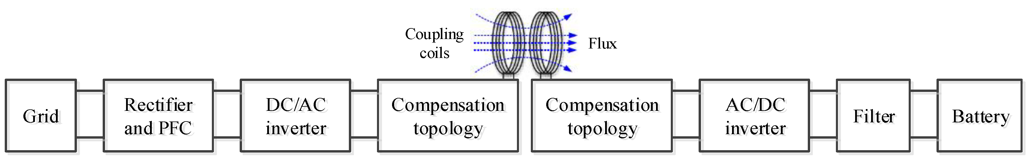
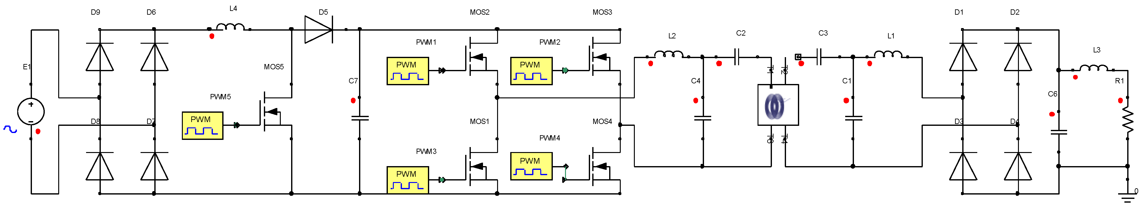
According to regulations on the power of SAE J2954, WPT1 (Wireless Power Transmission level 1) with 3.7 kW WCS is selected as a design product. The overall system is composed as shown in Figure 1. The primary side consists of a grid input, a power factor correction (PFC) circuit, an inverter, a primary compensation topology, and a primary coil, which are arranged on the ground; the secondary side is composed of a secondary coil, a secondary compensation topology, a rectifier, a filter and the battery arranged at the chassis of vehicle. The common part of primary and secondary side is the coupling coils, between which energy is transmitted through a coupling magnetic field.

Figure 1. Components of WCS.

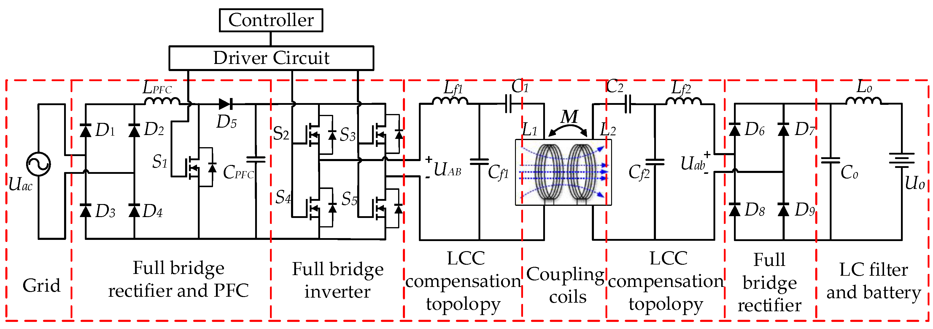
The overall circuit structure is built according to the components in Figure 1, as shown in Figure 2. The input voltage of system is 220V AC. After rectification and boosting by PFC, the output DC voltage of PFC reaches 425V, and then the inverter is used to change the 425V DC voltage to 85 kHz AC voltage. Then, the energy is coupled through the coupling coils and compensation circuit to rectifier and filter of the secondary side. For the on-board battery, the charging DC rated voltage is 400V, and the maximum output power of WCS is required as 3.7 kW. According to the respective function in Figure 2, parameters of these electrical modules are designed and determined.

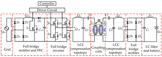
Figure 2. Circuit structure of WCS.

2.1. Design of the Input and Output Electrical Modules

2.1.1. Design of Rectifier

The primary single-phase rectifier consists of four diodes in Figure 2. The diodes of the rectifier are determined by the input voltage U_ac and effective input current I_RMS. I_RMS can be calculated by the following formula:

$${{\displaystyle I}}_{RMS}=\frac{P_0}{\eta U_{\mathrm{ac}}\cos \theta },$$

(1)

where P₀ is the maximum power of the WCS, η is the efficiency of the rectifier, and cosθ is the designed power factor of system. The Schottky diode as a reverse freewheeling diode is selected.

2.1.2. Design of PFC

The main function of PFC is to correct the power factor and improve the system’s efficiency. The Boost PFC is chosen to increase AC from 220 V to 425 V. Parameters of PFC are mainly including the boost inductor and PFC capacitor. The boost PFC utilizes the boost inductor to suppress current transient changes, so the boost inductor must be large enough to limit the output current ripple to a determined range, which is 15%. The peak of current flowing through the inductor can be obtained when reaching the maximum power and minimum voltage. The boost inductor L_PFC can be calculated as follows:

$$L_{\mathrm{PFC}}=\frac{\eta U_{\min }^2}{0.15f_s{P}_0}\left(1-\frac{\sqrt{2}{P}_0}{\eta U_{\mathrm{PFC}}}\right),$$

(2)

where U_PFC is the output voltage of PFC module, f_s is the switching frequency of mosfet, P_max is the maximum power and U_min is the minimum voltage after rectification.

The PFC capacitor C_PFC is used to reduce the ripple of output voltage, and it can be calculated by the following formula:

$$C_{\mathrm{PFC}}=\frac{P_0}{2\pi \cdot 2f_{in}\Delta U_{\mathrm{PFC}}{U}_{\mathrm{PFC}}},$$

(3)

where f_in is the frequency of the public grid, and ΔU_PFC is the ripple of designed output voltage.

2.1.3. Design of Inverter

The 425V DC voltage from PFC needs to be inverted to 85 kHz AC voltage. The single-phase full-bridge inverter is selected as shown in Figure 2, which contains four mosfets (S₂, S₃, S₄, S₅,). The full-bridge inverter owns higher efficiency than half-bridge inverter. In addition, these mosfets need extra reliable drive circuit to send reliable signal.

2.1.4. Design of Filter

The battery has a requirement for the ripple of charging voltage and current, so the charging current must be filtered before charging the battery. A simple LC filter is selected, which has a wide applicability and small simultaneous impact. The inductor of the LC filter needs to not make the output current deteriorate. The inductor L_o and capacitor C_o can be selected according to the following formula [2]:

$$L_o=\frac{U_o^2}{2P_o{f}_o}(1-D_{out}),$$

(4)

$$C_o=\frac{L_o{I}_o^2}{U_{o\max }^2-U_o^2},$$

(5)

where D_out is the duty ratio and U_omax is the maximum output voltage.

The parameters of each component of system can be shown in Table 1:

Table 1. Main components of the input and output modules.

Parts	Structure	Parameters
PFC	Boost PFC	LPFC, CPFC
Filter	LC filter	Lo, Co

2.2. Design of Resonance Coupling Coils

2.2.1. Design of Coupling Coils

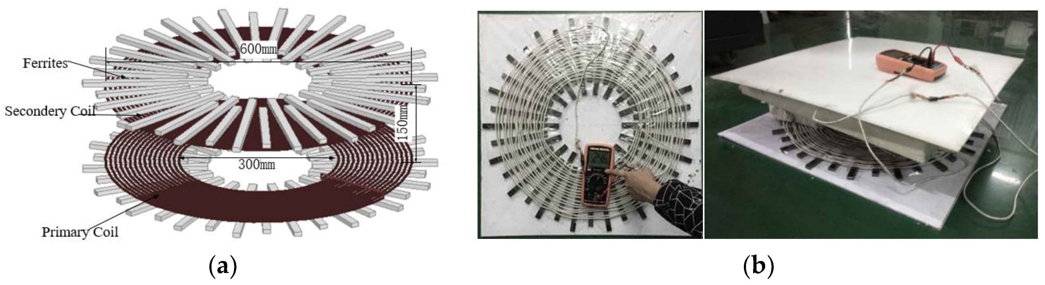
The primary and secondary coils with the same geometric size and shape are selected, and the Archimedes spiral coil arrangement with better anti-offset characteristics is selected. The ferrite is selected at a long and short staggered spoke layout. This layout can maintain the magnetic field strength at offset and save ferrite [22]. The coupling coils are made of multi-strand Litz wire, which can reduce the skin effect when the coils work at a high frequency. The 3D model of coupling coils with ferrite is shown in Figure 3.

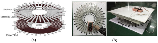
Figure 3. The coupling coils: (a) 3D model of coupling coils; (b) parameter measurement of coils.

Parameters of the coupling coils and ferrite are shown in Table 2. The three-dimensional model of coupling coils is established in ANSYS Maxwell. After the materials of coils and ferrite are correctly assigned, the electrical parameters of the entire coupling coils model can be efficiently extracted. For power coupling of the two coils, three main parameters are concerned, namely self-inductance, mutual inductance and coupling coefficient.

Table 2. Parameters of coils and ferrites.

Coil Attribute Name	Value/Type	Ferrites Attribute Name	Value/Type
Coil geometry	Planar spiral	Ferrite material	Ferroxcube 3C94
Outer diameter	600 mm	Long ferrite size	240 mm × 15 mm × 9 mm
Inner diameter	300 mm	Short ferrite size	180 mm × 15 mm × 9 mm
Number of turns	16	Long ferrite quantity	18
Conductor diameter	3.9 mm	Short ferrite quantity	18
Litz conductor	II(16AWG4×5X24/36)	Adjacent ferrite angle	10°

According to the design parameters, the coupling coils with a ratio of 1:1 is wound. The test LC instrument is used to measure the self-inductance and mutual inductance when the coils are flat, as shown in Figure 3b. It can be seen that the difference between the simulated and measured parameters is within 10% in Table 3, which verifies the accuracy of the three-dimensional model of coupling coils.

Table 3. Simulated and measured parameters of coils.

Parameters	Symbol	Simulated	Measured	Error (Percentage)
Self-inductance (µH)	L1L2	248.24	266	17.76 (6.7%)
Mutual inductance (µH)	M	95.74	100	4.26 (4.3%)
Coupling coefficient	k	0.3902	0.36	0.0302 (8.3%)

2.2.2. Design of Compensation Topology

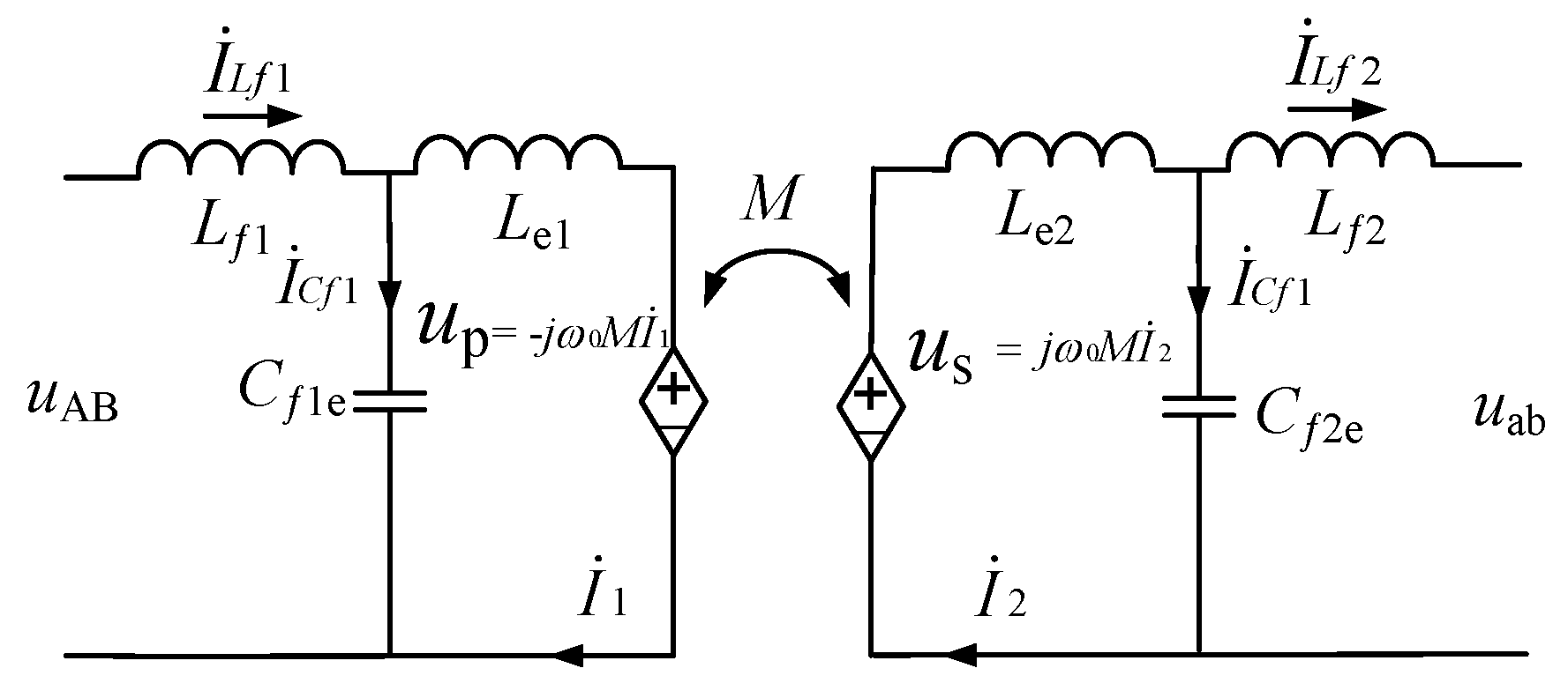
The compensation network adopts a bilateral LCC topology (Figure 4). A satisfying feature of LCC is that it can behave as a constant current source over a large load range when working at or close to the resonant state. It can reduce the difficulty of controlling when the battery is charging.

Figure 4. Equivalent circuit of LCC compensation topology network.

The transmit power P of system can be expressed as follows:

$$P={\dot{U}}_{AB}\cdot {\dot{I}}_{Lf1}=\frac{U_{AB}{U}_{ab}M}{2\pi f{L}_{f1}{L}_{f2}},$$

(6)

where U_AB is the input voltage and U_ab is the output voltage of compensation topology, and f is stands for resonant frequency. LCC circuits on both sides will magnetically resonate at f which is generally 85 kHz. The compensation inductor L_f1 and two capacitors C_f1 C₁ are calculated by Equations (7)–(9). Parameters of the compensation topology are equivalent, and the values are shown in Table 4 [23]:

$$L_{f1}=L_{f2}=\sqrt{\frac{k{U}_{AB}{U}_{ab}{L}_1}{{\omega }_{0}P}},$$

(7)

$$C_{f1}=C_{f2}=\frac{1}{{{\omega }_0}^2{L}_{f1}},$$

(8)

$$C_1=C_2=\frac{1}{{{\omega }_0}^2\left(L_1-L_{f1}\right)}.$$

(9)

Table 4. Parameters of compensation circuit.

Parameters	Symbol	Value
Compensation inductance	Lf1Lf2	42.4 µH
Compensation capacitance 1	Cf1Cf2	82.7 nF
Compensation capacitance 2	C1C2	19.1 nF

3. Modeling and Analysis of System

3.1. Modeling for Offset Coils

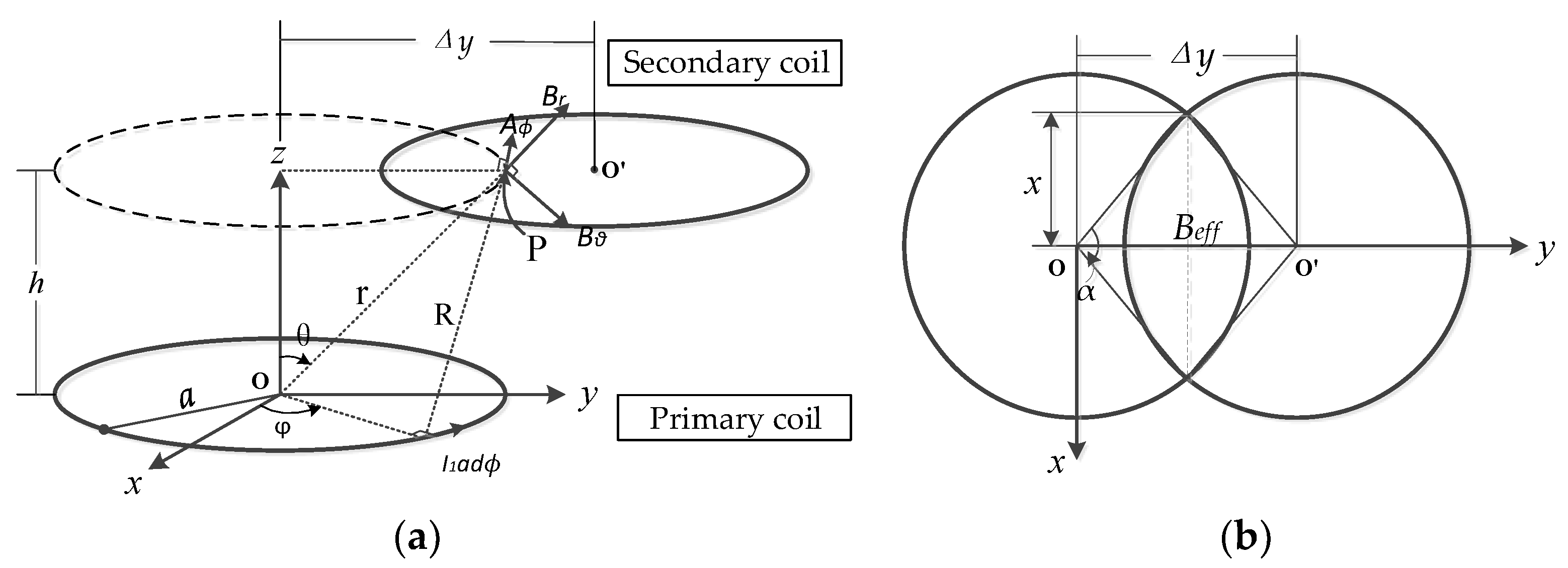
The magnetic vector potential A is introduced to study the characteristics of offset coils. Unlike the potential, A is not a measurable quantity and can be directly related to the physical quantity, which can help to solve the field distribution. A can be used to represent the interconnection of two axially aligned rings, and the magnetic vector potential around the closed path needs to be linearly integrated [24]:

$$\phi ={\displaystyle \int BdS}={\displaystyle \int (\nabla A)}dS={\displaystyle \oint Adl}.$$

(10)

In the WCS, when the excitation source is AC voltage, the ability of primary coil to cause an open circuit voltage in the secondary coil is called mutual inductance M, which is formally defined in electromagnetism:

$$M=\frac{N\phi }{I},$$

(11)

where $\phi$ is the magnetic flux connecting the two coils, which is usually a fraction of the total magnetic flux produced by the loosely coupling coils; N is the turns of coils; and I is the excitation current of the primary coil.

Figure 5 shows an offset diagram of the one turn coil. The horizontal deviation of the coil is Δy, and the magnetic vector potential at the point P on secondary coil is as follows:

$$A={\displaystyle \oint \frac{{\mu }_0{I}_{1}dl}{4\pi R}},$$

(12)

where μ₀ is the transmission efficiency. According to the geometric relationship, the lateral distance x and the angle α can be obtained:

$$x=\sqrt{a^2-{\frac{\Delta y}{4}}^2},$$

(13)

$$\alpha =2{\cos }^{-1}(\frac{\Delta y}{2a}).$$

(14)

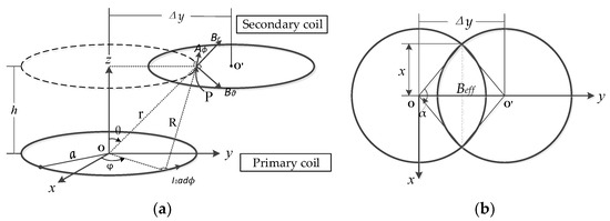
Figure 5. Offset diagram: (a) coordinate view; (b) top view.

The effective area that captures the primary flux can be interpreted as the intersection parts of coils, B_eff. The overlapping area of the primary and secondary coil is easily obtained from the relationship between Δy and the radius a:

$$B_{eff}=2\frac{1}{{180}^{°}}{\cos }^{-1}(\frac{\Delta y}{2a})\pi a^2-2(\frac{\Delta y}{2a^2})[\sqrt{\frac{{(\Delta y)}^2}{{(2a^2)}^2+1}}]a^3.$$

(15)

Then, we can get the relationship of mutual inductance:

$$M=(\pi a^2)(B_{eff})\frac{{\mu }_0}{\pi {(\sqrt{a^2+h^2})}^3}.$$

(16)

For the primary and secondary coils with N turns, the total mutual inductance can be calculated by superposition of the individual flux:

$$M={\displaystyle \sum _{i=1}^N{\displaystyle \sum _{j=1}^N\frac{{\mu }_0(\pi a_i{}^2)(B_{eff,j})}{\pi (\sqrt{a_j{}^2+h^2})}}}.$$

(17)

It can be seen from Equation (17) that M is mainly related to the geometrical quantities such as shape, size and relative position of the coil. When the offset Δy increases, M decreases, which may affect the transmission efficiency. The relationship between the coupling coefficient k and the self-inductance of coils is as follows:

$$k=\frac{M}{\sqrt{L_1{L}_2}}.$$

(18)

According to Equation (18), when the change of self-inductance L₁L₂ caused by the offset is ignored, the coupling coefficient k is proportional to the mutual inductance. When the offset increases, the ability to transmit electromagnetic fields reduces.

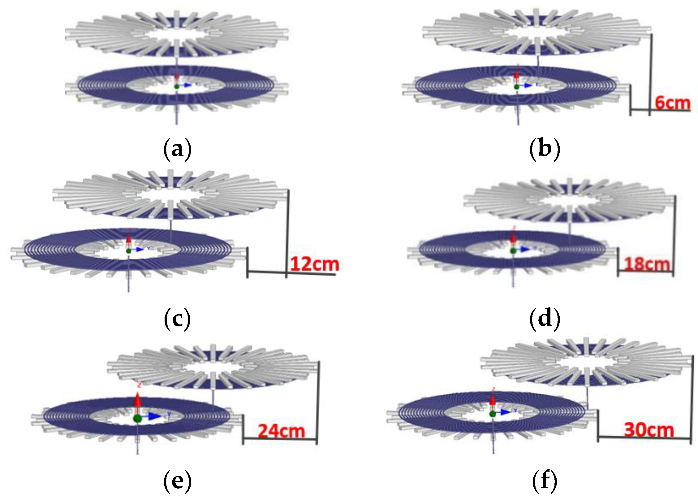
Due to coils mounted on the floor in front of vehicle, only the lateral offset of secondary coil in the vehicle coordinate system is considered. Coil models with full alignment, 10%, 20%, 30%, 40% offset and 50% offset are built in Maxwell, as shown in Figure 6. The self-inductance of the primary coil and secondary coil, and the mutual inductance between two coils are obtained by simulation. Thus, the coupling coefficient can be calculated.

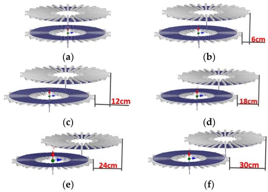
Figure 6. Relative position of coils: (a) alignment; (b) 10% offset—60 mm; (c) 20% offset—120 mm; (d) 30% offset—180 mm; (e) 40% offset—240 mm; (f) 10% offset—300 mm.

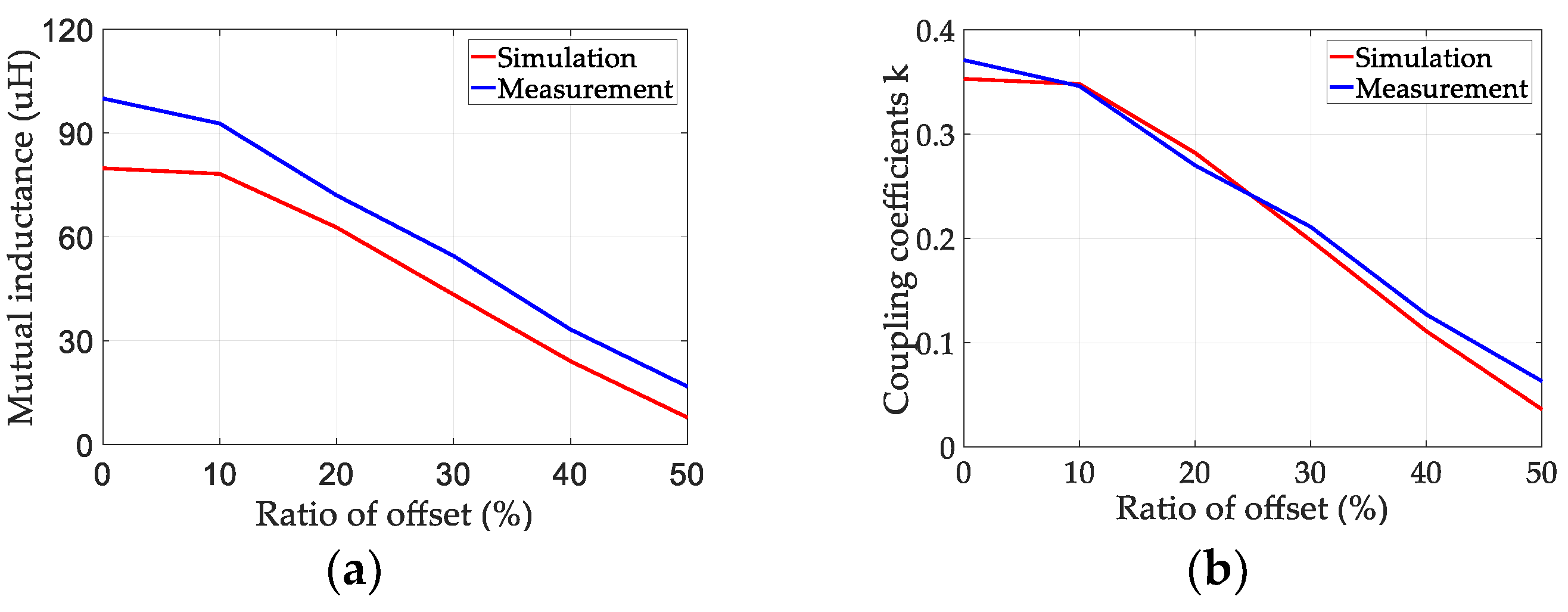
The experimental results of M and k at different offsets are compared with the simulated results, as shown in Figure 7. M obtained by the experiment is slightly larger than the simulation results. A part of Litz wire is reserved for the convenience of connecting the instrument, so that the self-inductance is larger than the actual value. As the offset increases, M and k of the experiment and simulation results show a downward trend, which is consistent with the analysis results.

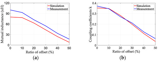
Figure 7. Comparison of simulation and measurement: (a) mutual inductance; (b) coupling coefficients.

3.2. Modeling for the Circuit

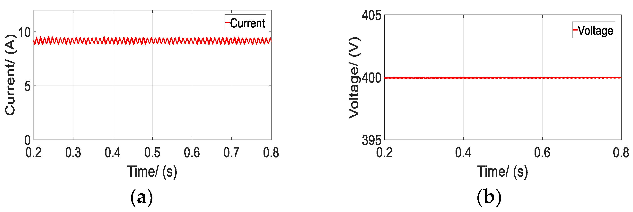
Based on the design parameters above, the circuit model of WCS is built by Simplorer, and co-simulate with coils established in Maxwell, as shown in Figure 8. The control circuit is used to control the inverter to generate the required voltage and constant sinusoidal current in the primary coil. The four mosfets are controlled by PWM (Pulse Width Modulation) and have a duty cycle of 0.5. The simulation results of the output voltage and charging current are 400 V and 9.25 A respectively, as shown in Figure 9, while the output power reaches the designed value of 3.7 kW.

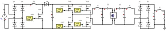
Figure 8. Circuit of the WCS.

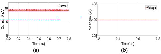
Figure 9. Charging parameters: (a) Current; (b) Voltage.

3.3. Modeling for the Vehicle Body

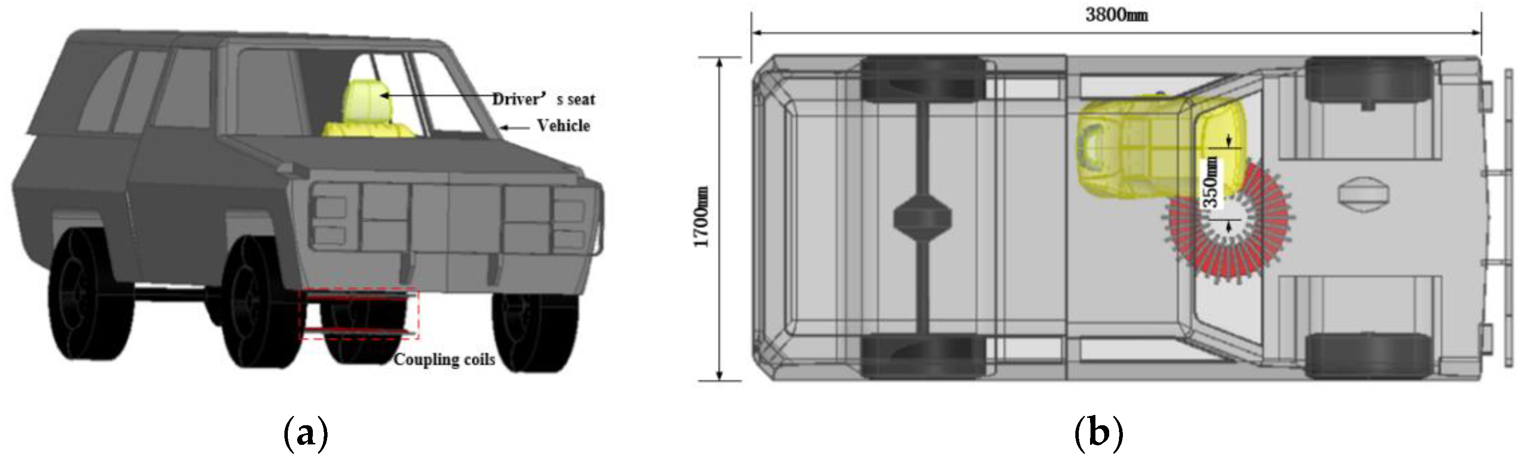
A general vehicle model with a driver seat is selected as the vehicle body model. The model is built according to the actual vehicle size in the 3D modeling software Catia, which includes a 1.5 m × 1.5 m × 1 mm metal plate as the vehicle mimic floor pan. Finally, the coupling coils and the whole vehicle body model are integrated and arranged as shown in Figure 10. The coils are located at the lower right of the driver seat and is close to the front axle of the vehicle.

Figure 10. 3D model of the vehicle body: (a) Side view; (b) Top view.

4. Simulation and Analysis of Magnetic Field Distribution

4.1. Magnetic Field Distribution for Alignment Coils

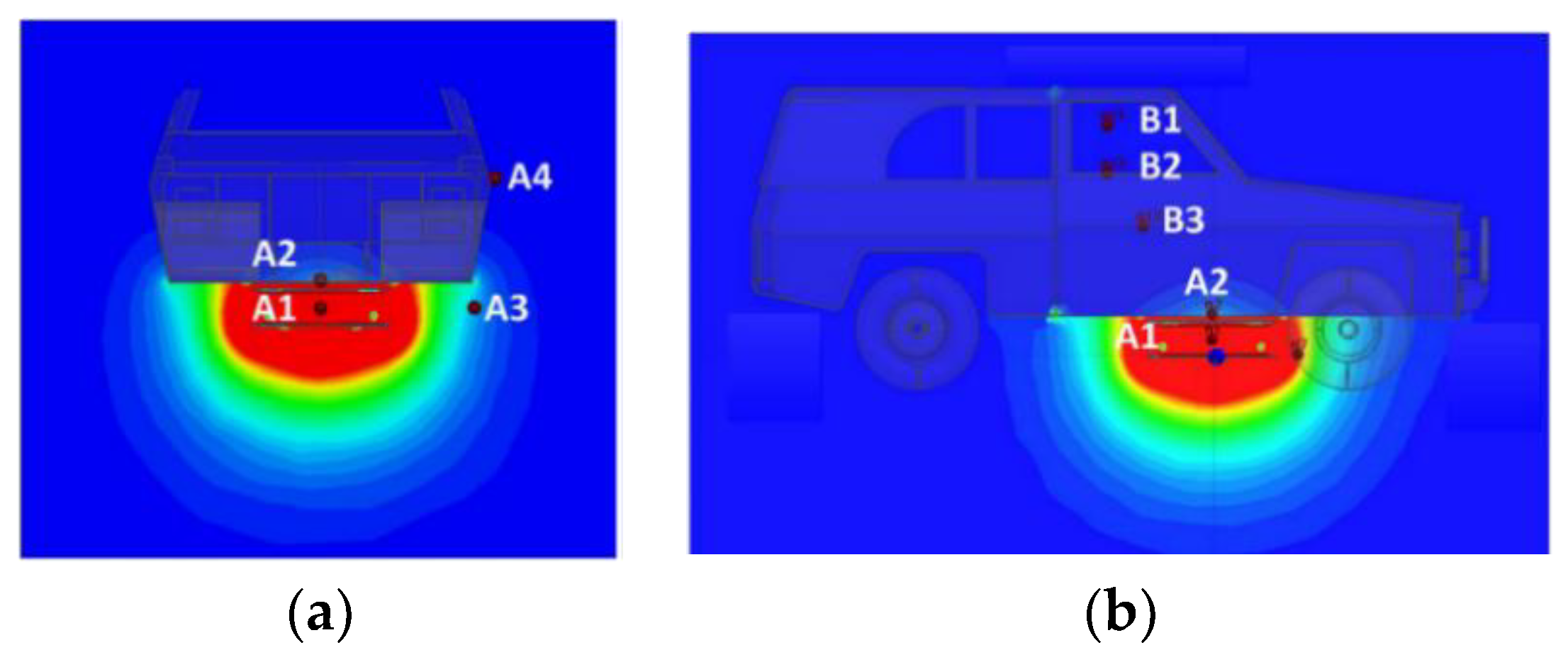
In order to analyze the magnetic field distribution around the vehicle when WCS is working, the space is divided into four geometric areas as defined by SAE J2945, namely 1, 2a, 2b, 3, shown in Figure 11. Area 1 is the main area of energy coupling, and it is necessary to focus on the magnetic field distribution of other areas. Four points (A1, A2, A3, A4) in different regions are selected as our test points in Figure 11a. They are located at the axial plane of the coupling device, and strictly follow the guidelines of SAE J2954. Since drivers stay in the cab for a long time, it is necessary to secure the cab’s magnetic field in area 3. The SAE J2954 also gives test points for the magnetic field at the driver’s seat in area 3. It is necessary to observe the strength of the head (B1), chest (B2) and cushion (B3) at each seat. The measurement should be repeated for each combination of alignment and offset conditions. The relative position of test points are shown in Fig 11b, and each test point is 10 mm above the surface and is in the axial plane of the seat.

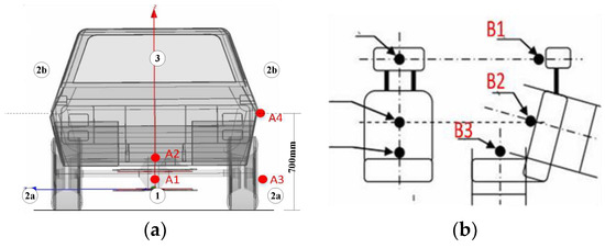
Figure 11. Position of test points; (a) position of A1, A2, A3, A4; (b) position of B1, B2, B3.

The electromotive force (EMF) standard and pacemaker/ implanted medical device (IMD) limit for public applications are given in SAE J2954, while meeting the requirements of ICNIRP 2010. The limits are shown in Table 5. Considering that the simulation reflects a transient magnetic field characteristic, we take the peak limits as reference.

Table 5. General public basic restriction of magnetic field.

Limits	Area	Root-Mean-Square Limit	Peak Limit
EMF Standard	2a, 2b, 3	27 uT or 21.4 A/m	38.2 uT or 30.4 A/m
Pacemaker/IMD Limit	3, 2b	15 uT or 11.9 A/m	21.2 uT or 16.9 A/m
Pacemaker/IMD Limit	2a	29.4 uT or 23.4 A/m	41.6 uT or 33.1 A/m

The current excitation of WCS extracted in Simplorer was respectively injected into the primary and secondary coils, and then we obtained the simulation results of magnetic field in Maxwell. When the coil is aligned, the simulation results are shown in Figure 12. The magnitude of the magnetic field at each test point are shown in Table 6.

Figure 12. Magnetic field of aligned coils: (a) front view; (b) right view.

Table 6. Position and magnetic field strength of test points.

Test Point	Coordinates (mm)	Magnetic Field Strength (A/m)
A1	(0,0,75)	1223
A2	(0,0,210)	13.07
A3	(0,740,75)	14.15
A4	(0,840,700)	3.22
B1	(550,0,1200)	0.21
B2	(550,0,950)	0.15
B3	(360,0,670)	0.72

From the results, it can be seen that magnetic field strength of A1 can reach 1223 A/m when the coils are perfectly aligned, and the magnetic field strength of all positions does not exceed the limit except for the effective region. The magnetic field strength of test points outside the vehicle is significantly larger than those inside the vehicle. Except for A1 in the working area, the magnetic field strength at A3 on the lower right side of the vehicle can reach 14.15 A/m. Although A3 does not exceed the standard limit, it has a higher risk of exceeding the limits.

4.2. Magnetic Field Distribution for Offset Coils

4.2.1. Current of Offset Coils

According to the analysis of LCC compensation topology, the primary current is only related to the input voltage. When the two resonant coils are not aligned, magnitude of the primary current does not change. However, the ability of secondary coil to receive a magnetic field changes due to the offset, so the current of secondary coil also changes. Current of the secondary coil can be expressed by the following formula:

$${\dot{I}}_2=\frac{U_{ab}}{2\pi f{L}_{f2e}}\angle 0^{°},$$

(19)

$${\dot{I}}_{Lf2}=\frac{k\sqrt{L_1{L}_2}{U}_{AB}}{j{\omega }_0{L}_{f1e}{L}_{f2e}}\angle -{90}^{°}.$$

(20)

Impedance of the rectifier and battery in the secondary circuit is equivalent to R_eq, and the output voltage U_ab can be expressed by the formula:

$${\dot{U}}_{ab}={\dot{I}}_{Lf2}·R_{eq}=\frac{k\sqrt{L_1{L}_2}}{j{\omega }_0{L}_{f1e}{L}_{f2e}}·R_{eq}\angle -{90}^{°}.$$

(21)

Thus, the current of secondary coil can be expressed:

$${\dot{I}}_2=\frac{k\sqrt{L_1{L}_2}}{{{\omega }_0}^2{L_{f1e}{L}_{f2e}}^2}·R_{eq}\angle -{90}^{°}.$$

(22)

It can be known that R_eq, L_f1e, L_f2e, and ω₀ are constant, so the current I₂ is positively correlated with the coupling coefficient k, the primary inductance L₁, and the secondary inductance L₂.

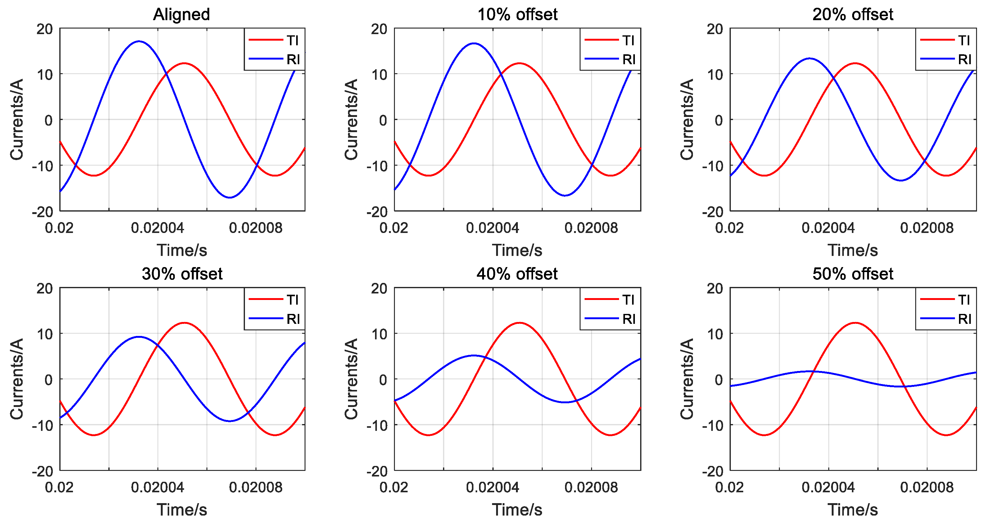
Currents of primary and secondary coils can be obtained by Simplorer, shown in Figure 13, where TI is the current of primary coil and RI is the secondary current. It can be seen that the primary current lags the secondary current by 90 degrees. When the coils are offset, the primary coil current is almost constant, and the secondary coil current is gradually reduced.

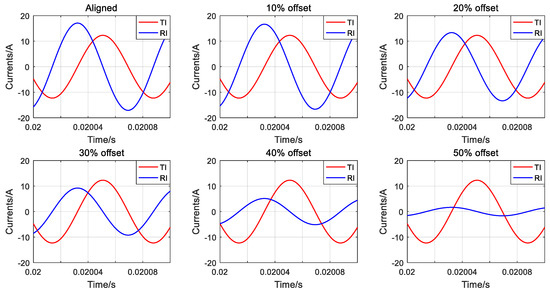
Figure 13. Currents of primary and secondary coils.

4.2.2. Phase of the Primary Current

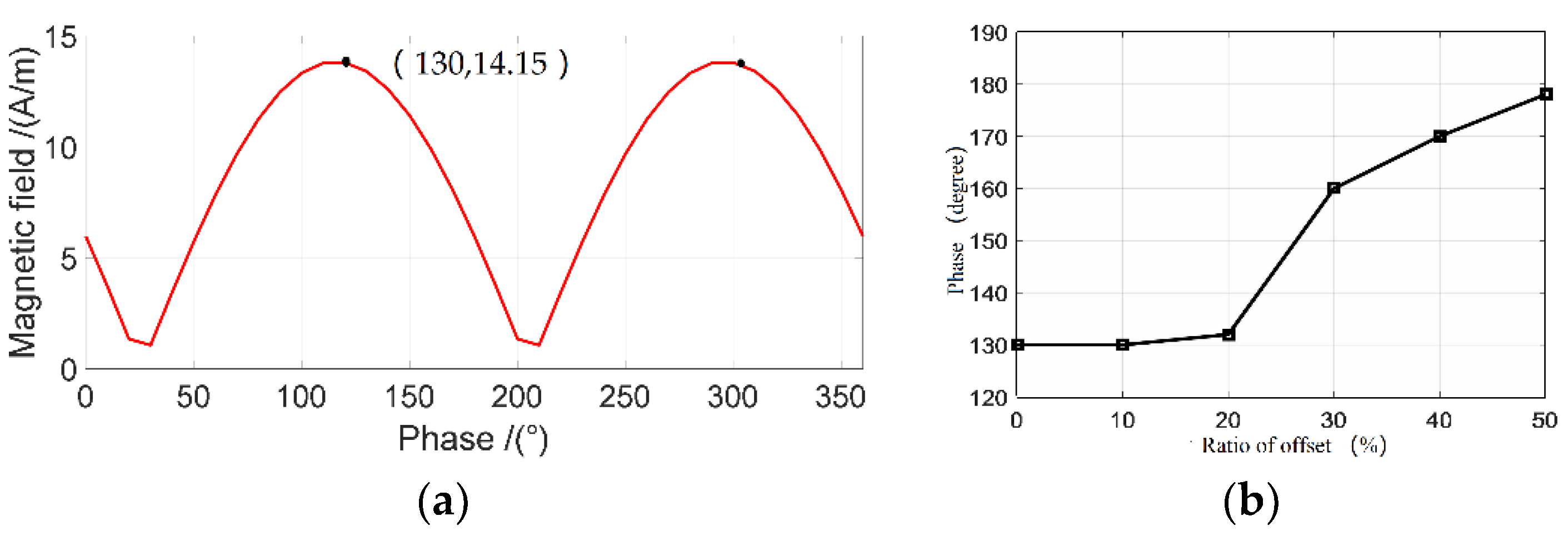
Due to the characteristics of coupling coils, when the current on primary side changes, the secondary current also changes along with resonance phenomenon, and lags behind the primary current. The transmission from primary side to the secondary side is a cyclical process, and the magnetic field is a superposition of field generated by currents in the primary and secondary coils. Therefore, the maximum instantaneous magnetic field strength occurs in one cycle. Figure 14a shows the phase fluctuation of primary current corresponding to the risk point A3 when the coils are completely aligned. The maximum magnetic field at A3 is at a phase of 130 degrees of the primary current.

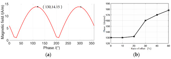
Figure 14. Phase of the primary current: (a) phase of the primary current at test point A3; (b) relationship between the offset and the phase of the maximum magnetic field.

Similarly, the five phases with various offsets can be obtained, and the primary current phase corresponding to the maximum magnetic field is shown in Figure 14b. The principle of coupling shows that as the offset increases, the primary current phase of the maximum magnetic field is different, which shows an increasing trend within the offset range. The simulation of magnetic field distribution is based on the current phase corresponding to the maximum magnetic field.

4.2.3. Magnetic Field Distribution of Offset Coils

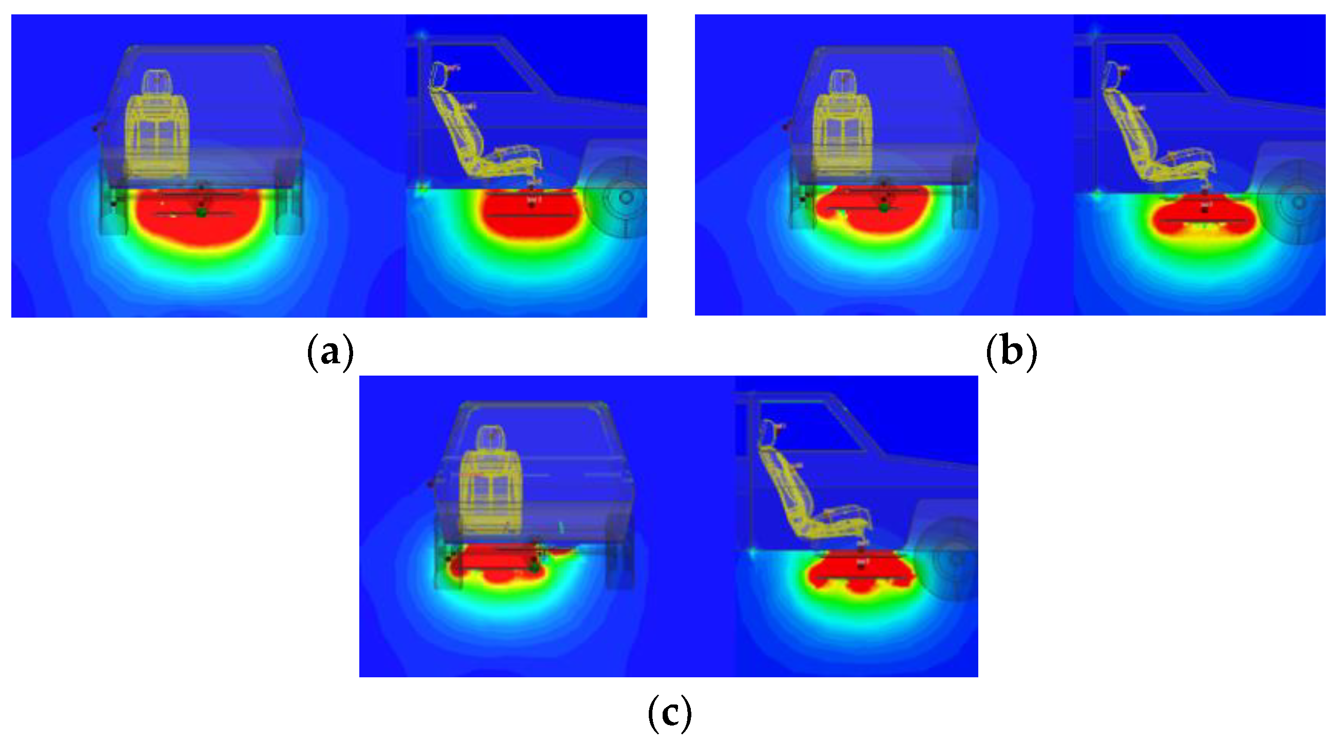
Similar to the simulation results of alignment, the magnetic field distribution under different offset conditions are obtained, the result of maximum magnetic field distribution is shown in Figure 15. The axial plane of coils and the central axis of driver’s seat are selected as an observation plane. It can be seen that as offset increases, the magnetic field of axial plane of coils moves to the left. The distribution of magnetic field becomes irregular, and the area of a red region with a larger magnetic field also decreases, which may reduce the transmission efficiency. Correspondingly, the energy transmission area will move towards the axial plane of the seat. Areas with high magnetic field strength are mainly distributed under the chassis of the vehicle, and the magnetic field strength inside the vehicle body is much smaller. Figure 16 is obtained based on the magnetic field strength of six test points in five offsets except A1.

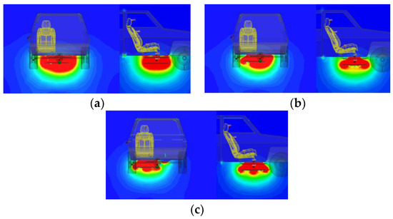
Figure 15. Magnetic field distribution: (a) 10% offset—60 mm; (b) 30% offset—180 mm; (c) 50% offset—300 mm.

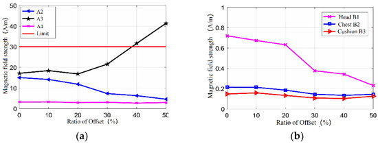
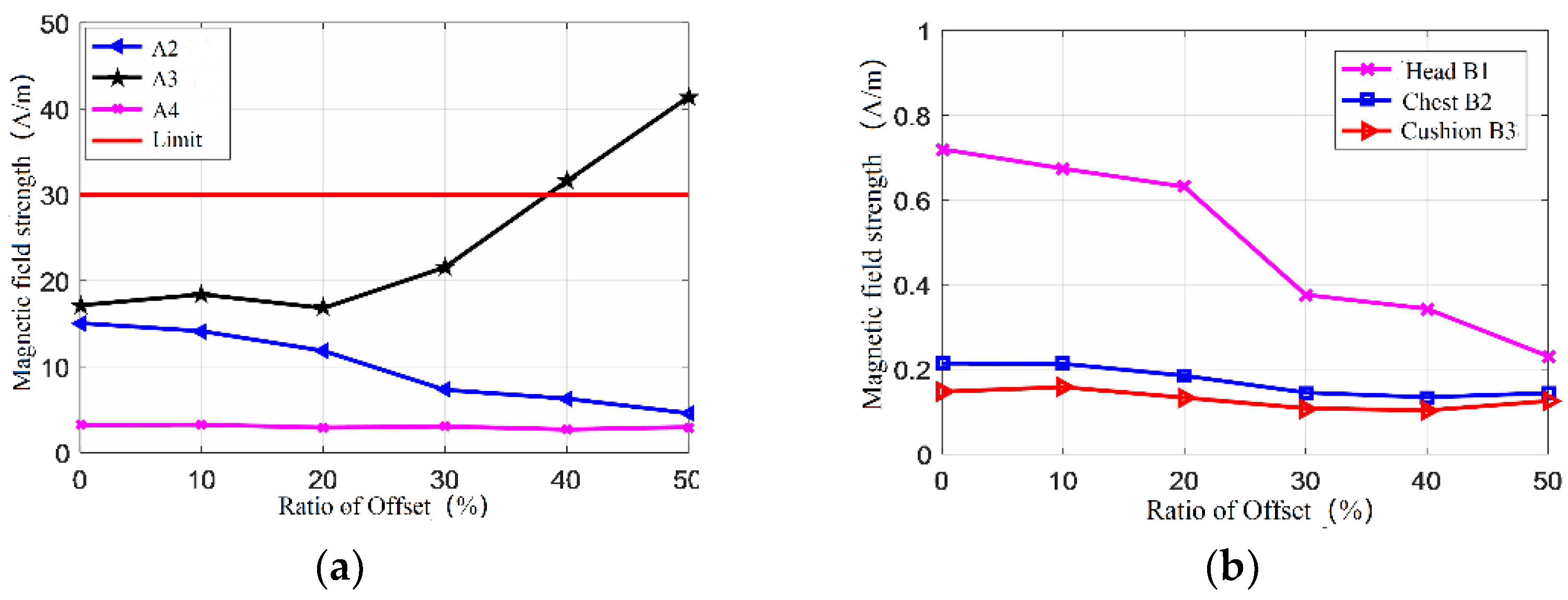
Figure 16. Magnetic field strength: (a) test points of A2, A3, A4; (b) test points of B1, B2, B3.

Apart from A1 located in the transmission region, the magnetic field strength at A3 is larger than 30.4 A/m required by SAE J2954 at 40% offset and 50% offset. The magnetic field strength under other offsets are not exceeded. The effective magnetic field between the coupling coils decreases with the increase of the offset. When the offset ratio exceeds 10%, the magnetic field of A2 drops greatly, which is close to a negative correlation. When the offset is less than 20%, the field at A3 is nearly invariable. However, after this ratio is exceeded, the amount of magnetic field leakage continues to increase, and after more than 40%, the exceeding strength appears. As the offset increases, the primary coil on the ground gradually approaches A3, making A3 close to the energy transmission region. However, while A4 is far away the coils, the offset has little effect on it. Since the vehicle body is an enclosed conductor, the magnetic field strength of B1, B2, B3 has little fluctuation with the offset, and maintains less than 1 A/m.

4.3. Magnetic Field Generated by Sideband Current and Harmonic Current

4.3.1. Sideband Current

With the help of LCC, the coupling coils resonate at a specific frequency of 85 kHz. At the specific frequency, energy can be transferred with a higher efficiency. However, the resonant frequency fluctuates at a small range when the system works. Thus, a lot of sideband currents around the resonant current exist that can affect the magnetic field.

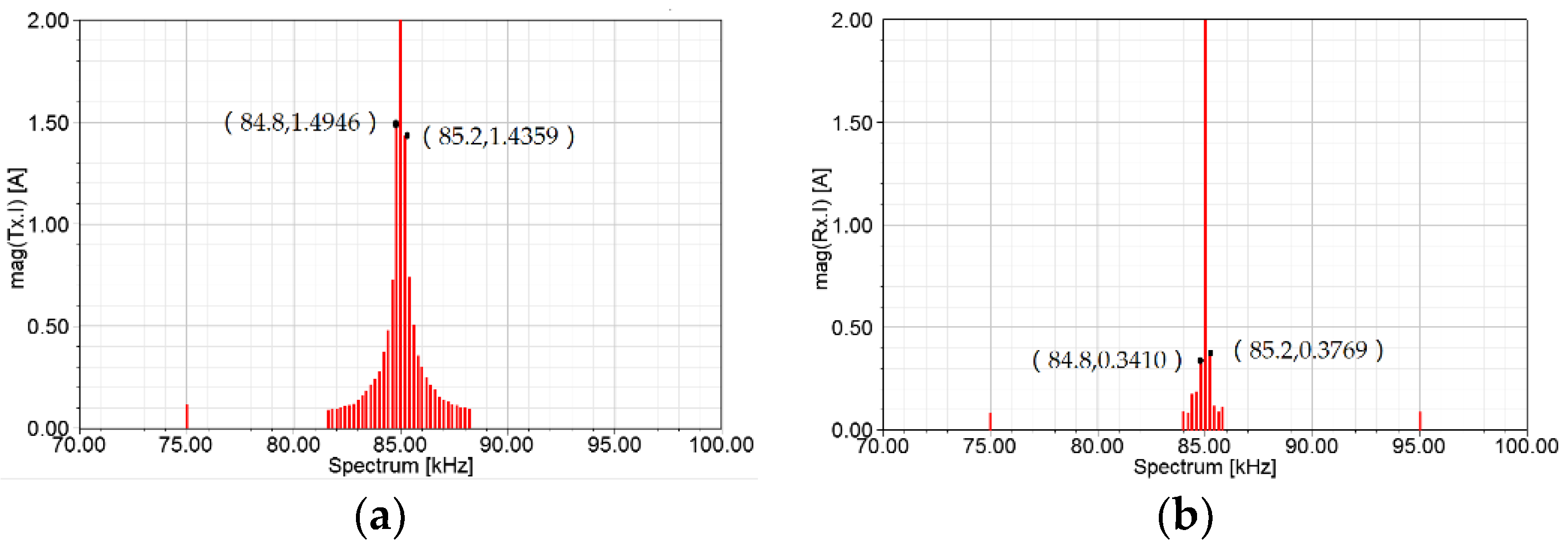
The corresponding current spectrum with the frequency step 200 Hz in the primary and secondary coil is obtained as shown in Figure 17. The current reaches a peak at a frequency of 85 kHz and a large amount of sideband currents exist around 85 kHz. The sideband currents on the primary side are much more than the secondary side, and the current’s amplitude is greater at the same frequency.

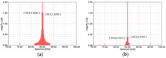
Figure 17. Current spectrum of coupling coils: (a) current spectrum of primary coil; (b) current spectrum of secondary coil.

The harmonic of primary and secondary side at 84.8 kHz and 85.2 kHz are respectively extracted and injected into the Maxwell, and the magnetic field distribution is obtained as shown in Figure 18 and the results are recorded in Table 7. For A1 located in the working region, the magnetic field strength at A3 is the highest among these test points, reaching 1.75 A/m and 1.76 A/m at 84.8 kHz and 85.2 kHz. From the previous analysis, the magnetic field strength at the risk point A3 has reached 14.15 A/m. Thus, when considering the superposition of the magnetic field generated by the sideband currents, the total magnetic field strength at A3 will be slightly larger than the simulated result, and the risk of exceeding the limit will increase, which needs to be taken seriously. Then, the magnetic generated by current at sideband frequency should not be ignored in real practice.

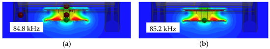
Figure 18. Magnetic field distribution of harmonic current: (a) harmonic current at 84.8 kHz; (b) harmonic current at 85.2 kHz.

Table 7. Magnetic field strength at test points (A/m).

Frequency	A2	A3	A4	B1	B2	B3
84.8 kHz	0.86	1.75	0.22	0.02	0.03	0.13
85.2 kHz	0.83	1.76	0.22	0.02	0.03	0.13

4.3.2. Odd Harmonic Current

Other than the sideband currents at a frequency of 85 kHz, there are also non-negligible frequency doubling harmonics, including odd and even harmonics. The four power devices in inverter for WCS is controlled by PWM, and the output voltage is a pulse width modulated square wave. The large du/dt and di/dt can induce abundant harmonic currents in the primary and secondary current. Harmonics can not only bring serious EMI, but also affect the magnetic field distribution. The odd harmonic currents are large and the even harmonics are nearly zero; therefore, the influence of odd harmonics on the WCS is mainly considered here. The higher harmonics of coupling coils is gradually reduced, and the harmonic is negligible after the 5th harmonic. Only 3th and 5th current harmonics are considered here at five cases for offset, as shown in Table 8.

Table 8. Harmonic currents with the offset (A/m).

Offset	Primary 3rd Harmonic	Secondary 3rd Harmonic	Primary 5th Harmonic	Secondary 5th Harmonic
0	0.5399	0.3724	0.1034	0.1034
10%	0.5291	0.3661	0.1020	0.1060
20%	0.5140	0.3611	0.1103	0.1056
30%	0.5776	0.3681	0.1286	0.1191
40%	0.7801	0.3211	0.954	0.1152
50%	0.9573	0.1659	0.736	0.0625

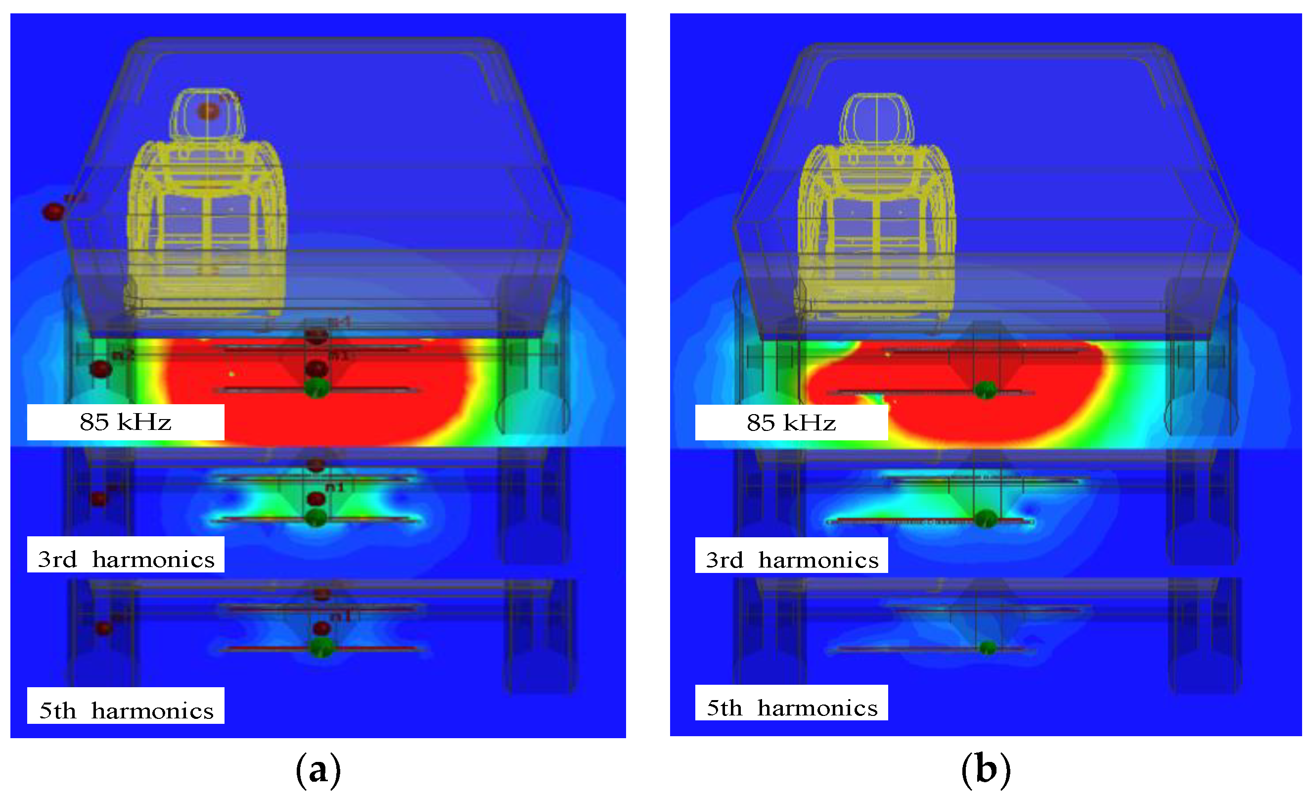
The LCC compensation topology can suppress the harmonics in a way, so the overall harmonic currents are small. The 3rd harmonic current of the secondary coil is greater than that of the primary coil, and, as the offset increases, the primary harmonic current decreases at the beginning and then increases later. The odd harmonic currents are injected into the model when the coils are aligned, and a comparison of the magnetic field distribution of the 3rd and 5th harmonics with the fundamental magnetic field can be obtained, as shown in Figure 19.

Figure 19. Comparison of different magnetic field: (a) alignment; (b) 30% offset.

4.3.3. EMI Noise Current

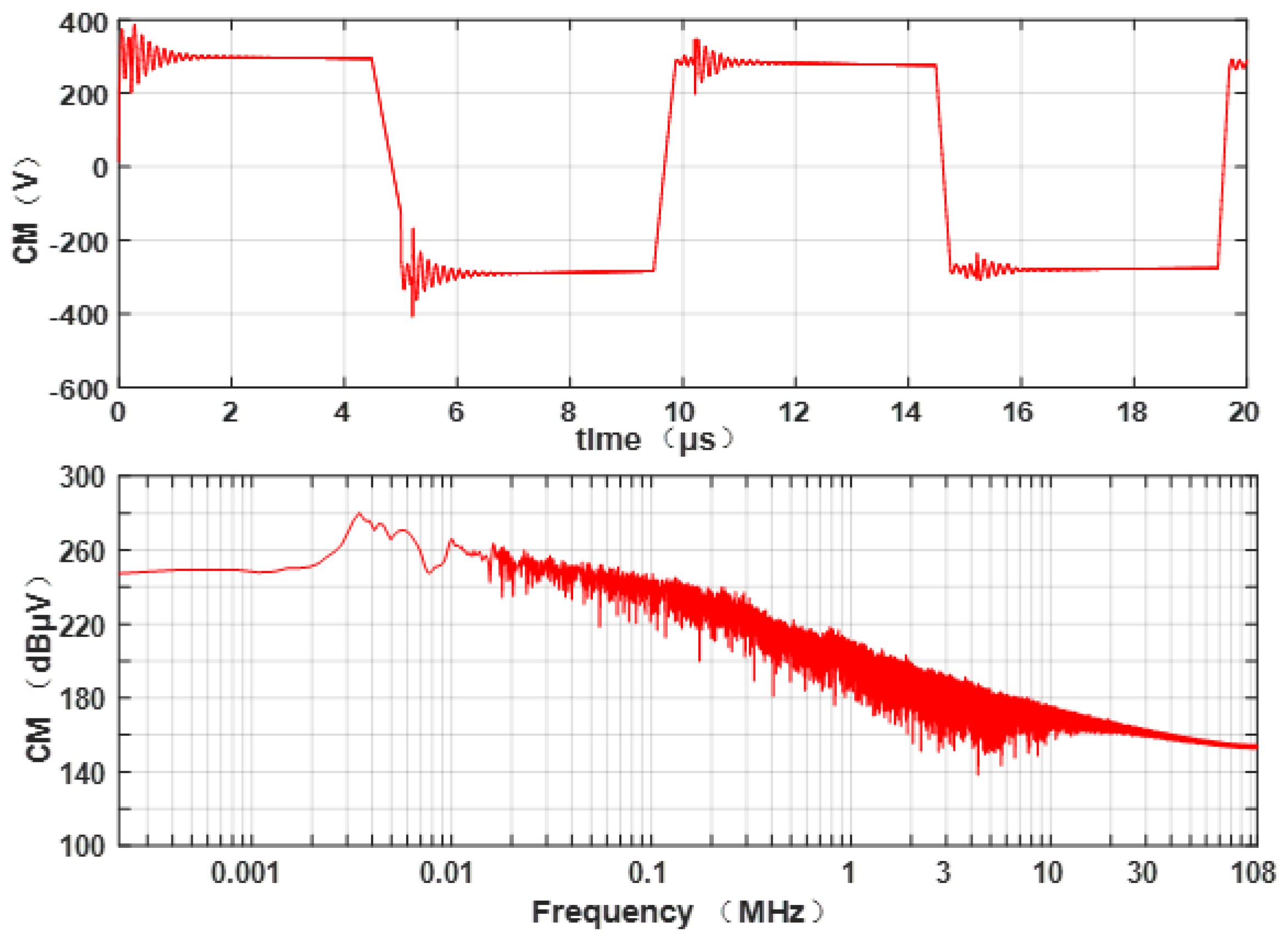
When switching devices such as mosfet and diode are switched on and off, they will produce large voltage change rate du/dt and current change rate di/dt, which will generate abundant high frequency signals, as shown in Figure 20, thus forming conduction and radiation electromagnetic emission. Magnetic field distribution of a vehicle with WCS is shown in Figure 21.

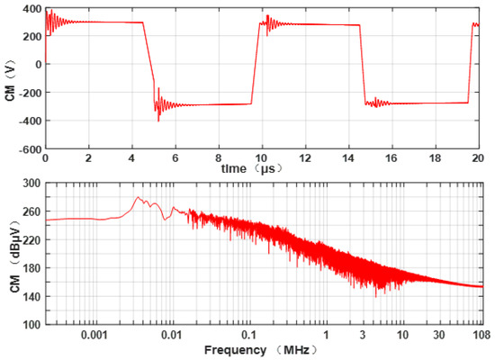
Figure 20. PWM signal of mosfet.

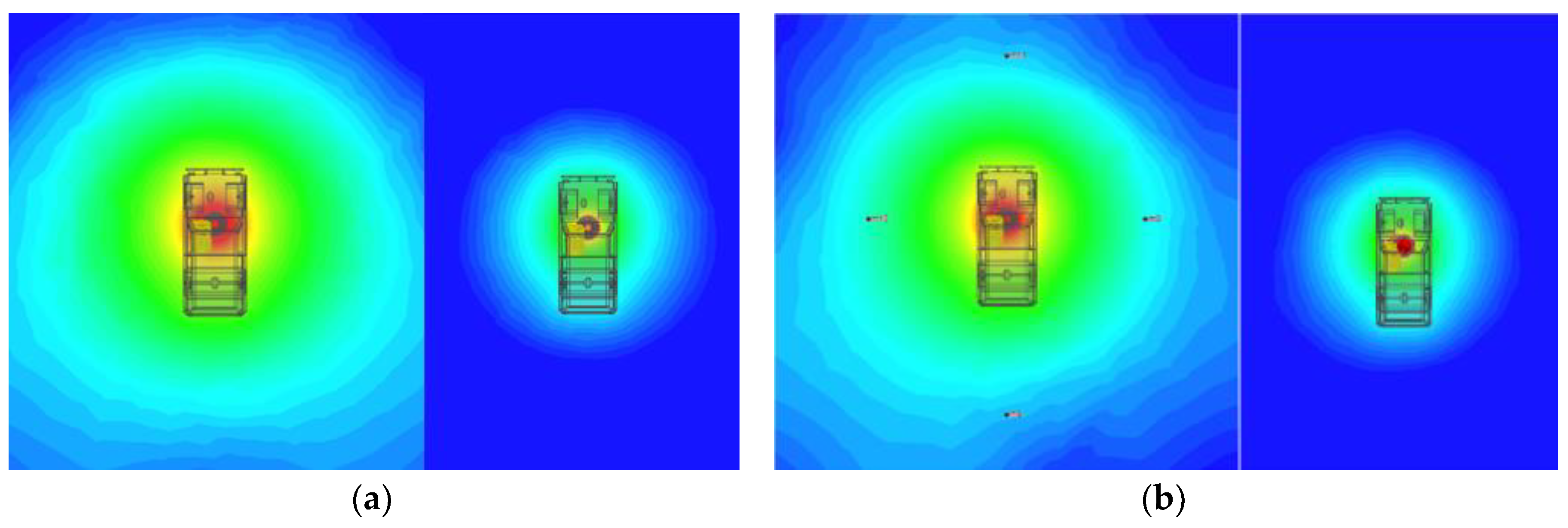
Figure 21. Far-field magnetic field distribution on fundamental current and third-order harmonic current: (a) alignment; (b) 30% offset.

Considering the magnetic field, radiation emission will also occur in a certain frequency range from 9 kHz to 108 MHz. The test points are located around the vehicle and three meters away from the body according to the requirement of SAE J2954, and the magnetic field distribution is shown in Figure 21.

Table 9. indicates that, at different frequencies, radiation emission values at four directions exceed the emission limit due to the large corresponding current. Radiation emission values under coil alignment and offset are consistent. Taking the operating characteristics of WCS into account, it is necessary to set protection to the wireless charging system to reduce the leakage magnetic field that might induce the radiation emission problems.

Table 9. Magnetic field strength at three meters around the vehicle.

Frequency	Front	Rear	Left	Right	Limit
85 kHz	88.79	87.45	97.63	98.29	28.5
255 kHz	76.23	60.37	69.89	70.24	18.95
85 kHz (30% offset)	86.12	84.24	91.23	92.11	28.5
255 kHz (30% offset)	76.07	60.19	69.47	69.67	18.95

5. Experiments

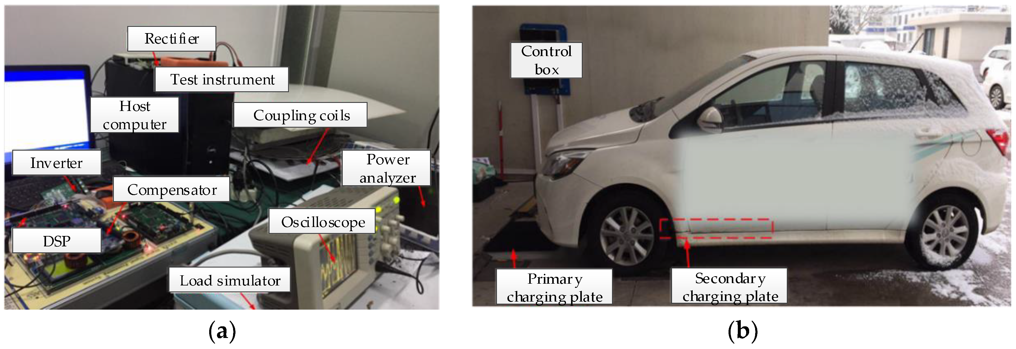
An experimental bench for the proposed 3.7 kW WCS is built as shown in Figure 22a. In order to validate the rightness and feasibility of simulation results, the proposed WCS is installed on the vehicle as shown in Figure 22a. When the EV is charging, the voltage and current of fast charging are 400V and 9.2 A, so the proposed WCS can charge normally.

Figure 22. Experiment condition: (a) wireless charging test bench; (b) experiment vehicle.

5.1. Magnetic Field Test for Alignment and Offset Coils

The measuring instrument used in the low-frequency magnetic field emission test is the ELT-400 from Narda, which is used to measure the omnidirectional magnetic field. When WCS works stably and the coupling coils are fully aligned, the magnetic field strength of the head, chest, cushion and low floor at 75 mm and 700 mm from the ground are measured. Figure 23 shows a testing for magnetic field strength at the antenna point, a 7.5 cm point from the ground and the seat point.

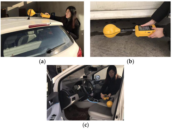
Figure 23. Testing at different points: (a) the antenna; (b) 7.5 cm point from the ground; (c) the seat.

These measurement results are compared with the simulation results in Table 10. It can be concluded that a position around the seat is less than 1 A/m, which is a safe level for the EMF exposure standard. Magnetic field strength at test points outside the vehicle are higher than the in-vehicle points, and the strength is the largest at a 7.5 cm point from the ground. It can be found that the experimental results are larger, while other sources of interference that exist outdoors are likely to be the influencing factor. A tiny error between the experimental results and the simulation results is allowed. Therefore, the experiment verifies the accuracy of the simulation model and the magnetic field simulation results in Maxwell.

Table 10. Experimental results are compared with simulation results (A/m).

Test Point	Experimental Results	Simulation Results	Difference
A2	14.55	13.07	0.52
A3	17.73	14.15	3.58
A4	1.85	3.22	1.37
B1	0.40	0.21	0.19
B2	0.38	0.15	0.23
B3	0.84	0.72	0.12

Magnetic field strength under different lateral offset conditions with respectively 60 mm, 120 mm, 180 mm, 240 mm, and 300 mm offsets are obtained by measurement. Three test points A2, A3 and A4 are selected to obtain the magnetic field strength under different offset conditions, as shown in Table 11. Each point takes three values, and finally takes the average value to be the magnetic field strength. From Table 11, it can be seen that the errors between experimental results and simulation results are 1.4 A/m, 2.1 A/m and 1 A/m, respectively. The prediction results of simulation are more accurate.

Table 11. Magnetic field strength at different offsets (A/m).

Offset	Experimental Results			Simulation Results
	A2	A3	A4	A2	A3	A4
60 mm	15.1	17.9	3.1	15.4	18.2	3.4
120 mm	11.9	17.2	3.2	12.3	17.8	3.3
180 mm	7.5	20.5	3.3	7.8	20.8	3.4
240 mm	6.3	30.7	3.0	6.5	31.2	3.3
300 mm	4.5	41.2	3.2	4.7	41.6	3.4
Error	A2	1.4 (3.1%)	A3	2.1 (1.6%)	A4	1 (6%)

5.2. Magnetic Field Test for Sideband Current and Harmonic Currents

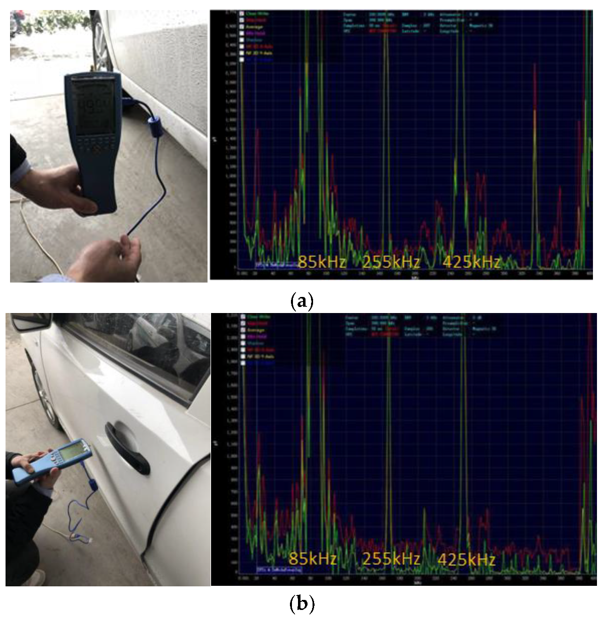
Magnetic field strength and magnetic induction intensity in the xy direction, yz direction and xz directions in a wide range of frequencies can be measured by the spectrum analyzer NF-5035. The magnetic induction intensity in different directions at 7.5 cm and 70 cm from the ground outside the vehicle were measured, as shown in Figure 24. The unit of magnetic field is pT. The red curve indicates the maximum value, the green one is the transient value, and the yellow one is the average value.

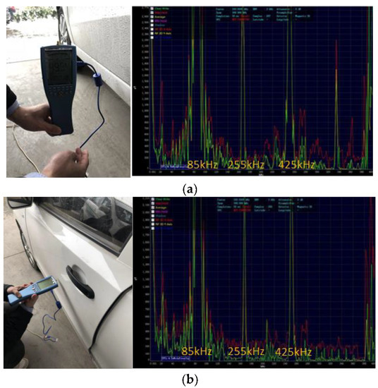
Figure 24. Magnetic induction intensity (pT) measurement of A3: (a) y-axis; (b) z-axis.

The magnetic field peaks appear at 85 kHz, 255 kHz (3th harmonic) and 425 kHz (5th harmonic) respectively. These frequencies are the multiples of 85 kHz, and the magnetic induction intensity reaches the highest at 85 kHz. The spikes of magnetic field also appeared outside the basic frequency, indicating that the side-band harmonics and odd harmonics also generate corresponding magnetic fields, which may have an effect on the measurement of magnetic field strength at test points. Therefore, when analyzing the magnetic field of WCS, it is necessary to comprehensively consider the magnetic field at the basic frequency, side-band frequency and the harmonic frequency. Adopting appropriate weighting factors can be a useful method. Magnetic field strength of sideband (84.8 kHz and 85.2 kHz) and harmonic currents (255 kHz and 425 kHz) with 30% offset are shown in Table 12.

Table 12. Magnetic field strength in the xy direction of sideband and harmonic currents with 30% offset (A/m).

Offset	Experimental Results			Simulation Results
	0 mm	180 mm	Error	0 mm	180 mm	Error
84.8 kHz	1.82	2.13	0.31	1.75	2.05	0.3
85.2 kHz	1.81	2.02	0.21	1.76	1.95	0.19
255 kHz	0.54	0.58	0.04	0.54	0.58	0.04
435 kHz	0.11	0.13	0.02	0.10	0.13	0.03

6. Conclusions

In this paper, 3.7 kW WCS is designed and modeled. In particular, the coupling coils are designed with detail and verified to guarantee the accuracy of the simulation model. Through simulation and analysis, it is verified that when the coils are completely aligned and in different offsets, the mutual inductance and coupling coefficient are significantly decreased. Along with the vehicle body, magnetic field distributions of the primary coil and the secondary coil at full alignment and five offsets are compared and analyzed at these typical test points. It is found that magnetic field strength of test point A3 located on the left side of the driver exceeds the limit due to the offset. Magnetic field strength at A3 is larger than 30.4 A/m required by EMF exposure standard at 40% offset and 50% offset. Finally, the sideband currents and the odd-multiplied harmonics generated by the power devices in WCS are analyzed, and the influence on the magnetic field distribution and the radiation emission caused by the higher harmonics are proved to show that there remains some risks in the system. The experimental results of magnetic field distribution have good agreement with simulation results.

References

- Ahmad, A.; Alam, M.S.; Chabaan, R. A Comprehensive Review of Wireless Charging Technologies for Electric Vehicles. IEEE Trans. Transp. Electrif. 2018, 4, 38–63. [Google Scholar] [CrossRef]
- Zhai, L.; Cao, Y.; Lin, L.; Zhang, T.; Kavuma, S. Mitigation Conducted Emission Strategy Based on Transfer Function from a DC-Fed Wireless Charging System for Electric Vehicles. Energies 2018, 11, 477. [Google Scholar] [CrossRef]
- Wang, Q.; Li, W.; Kang, J.; Wang, Y. Electromagnetic Safety Evaluation and Protection Methods for a Wireless Charging System in an Electric Vehicle. IEEE Trans. Electromagn. Compat. 2018. [Google Scholar] [CrossRef]
- De Santis, V.; Campi, T.; Cruciani, S.; Laakso, I.; Feliziani, M. Assessment of the Induced Electric Fields in a Carbon-Fiber Electrical Vehicle Equipped with a Wireless Power Transfer System. Energies 2018, 11, 684. [Google Scholar] [CrossRef]
- Laakso, I.; Hirata, A. Evaluation of the induced electric field and compliance procedure for a wireless power transfer system in an electrical vehicle. Phys. Med. Biol. 2013, 58, 7583. [Google Scholar] [CrossRef] [PubMed]
- Cai, C.; Wang, J.; Fang, Z.; Zhang, P.; Hu, M.; Zhang, J.; Li, L.; Lin, Z. Design and Optimization of Load-Independent Magnetic Resonant Wireless Charging System for Electric Vehicles. IEEE Access 2018, 6, 17264–17274. [Google Scholar] [CrossRef]
- Chung, Y.D.; Park, E.Y.; Lee, W.S.; Lee, J.Y. Impact Investigation and Characteristics by Strong Electromagnetic Field of Wireless Power Charging System for Electric Vehicle under Air and Water Exposure Indexes. IEEE Trans. Appl. Supercond. 2018, 28. [Google Scholar] [CrossRef]
- Kim, K.; Kim, J.; Kim, H. Evaluation of Electromagnetic Field Radiation from Wireless Power Transfer Electric Vehicle. In Proceedings of the ISAP, Okinawa, Japan, 24–28 October 2016; pp. 40–41. [Google Scholar]
- Ahn, S.; Kim, J. Magnetic Field Design for High Efficient and Low EMF Wireless Power Transfer in On-Line Electric Vehicle. In Proceedings of the 5th European Conference on Antennas and Propagation (EUCAP), Rome, Italy, 11–15 April 2011; pp. 3979–3982. [Google Scholar]
- Moon, H.; Kim, S.; Park, H.H.; Ahn, S. Design of a resonant reactive shield with double coils and a phase shifter for wireless charging of electric vehicles. IEEE Trans. Magn. 2015, 51, 8700104. [Google Scholar]
- Zhao, L.; Thrimawithana, D.J.; Madawala, U.K.; Hu, P.; Mi, C.C. A Misalignment Tolerant Series-hybrid Wireless EV Charging System with Integrated Magnetics. IEEE Trans. Power Electron. 2019, 34, 1276–1285. [Google Scholar] [CrossRef]
- Campi, T.; Cruciani, S.; Maradei, F.; Feliziani, M. Near-Field Reduction in a Wireless Power Transfer System Using LCC Compensation. IEEE Trans. Electromag. Compat. 2017, 59, 686–694. [Google Scholar] [CrossRef]
- Kim, S.; Park, H.; Kim, J. Design and Analysis of a Resonant Reactive Shield for a Wireless Power Electric Vehicle. IEEE Trans. Microw. Theory Tech. 2014, 62, 1057–1066. [Google Scholar] [CrossRef]
- Ding, P.; Bernard, L.; Pichon, L. Evaluation of Electromagnetic Field in Human Body Exposed to Wireless Inductive Charging System. IEEE Trans. Magn. 2014, 50, 1037–1040. [Google Scholar] [CrossRef]
- Chakarothai, J.; Wake, K.; Arima, T. Exposure Evaluation of an Actual Wireless Power Transfer System for an Electric Vehicle with Near-Field Measurement. IEEE Trans. Microw. Theory Tech. 2018, 66, 1543–1552. [Google Scholar] [CrossRef]
- Kim, H.; Song, C.; Jung, D.H. Coil Design and Measurement of Automotive Magnetic Resonant Wireless Charging System for High-Efficiency and Low Magnetic Field Leakage. IEEE Trans. Microw. Theory Tech. 2016, 64, 383–400. [Google Scholar] [CrossRef]
- ICNIRP. Guidelines for limiting exposure to time-varying electric and magnetic fields (1 Hz to 100 kHz). Health Phys. 2010, 99, 818–836. [Google Scholar]
- Campi, T.; Cruciani, S.; De Santis, V.; Maradei, F.; Feliziani, M. EMC and EMF Safety Issues in Wireless Charging System for an EV. In Proceedings of the AUTOMOTIVE 2017, Torino, Italy, 15–16 June 2017. [Google Scholar]
- Yang, G.; Zhu, C.; Song, K. Power Stability Optimization Method of Wireless Power Transfer System Against Wide Misalignment. In Proceedings of the IEEE Transportation Electrification Conference and Expo, Harbin, China, 7–10 August 2017. [Google Scholar]
- Campi, T.; Cruciani, S.; Feliziani, M.; Maradei, F. Magnetic field generated by a 22 kW-85 kHz wireless power transfer system for an EV. In Proceedings of the 2017 AEIT International Annual Conference, Cagliari, Italy, 20–22 September 2017; pp. 1–6. [Google Scholar]
- SAE TIR J2954. Wireless Power Transfer for Light-Duty Plug-In/Electric Vehicles and Alignment Methodology; 2016. Available online: https://www.sae.org/standards/content/j2954_201605/ (accessed on 26 January 2019).
- Lee, W.; Hong, Y.K.; Park, J.H.; Lee, J. A simple wireless power charging antenna system: Evaluation of ferrite sheet. IEEE Trans. Magn. 2017, 53. [Google Scholar] [CrossRef]
- Lu, F.; Zhang, H.; Hofmann, H.; Mi, C. A dual-coupled LCC-compensated IPT system to improve misalignment performance. In Proceedings of the 2017 IEEE PELS Workshop on Emerging Technologies: Wireless Power Transfer (WoW), Chongqing, China, 20–22 May 2017; pp. 1–8. [Google Scholar]
- Esteban, B.; Stojakovic, N.; Sid-Ahmed, M.; Kar, N.C. Development of mutual inductance formula for misaligned planar circular spiral coils. In Proceedings of the 2015 IEEE Energy Conversion Congress and Exposition (ECCE), Montreal, QC, Canada, 20–24 September 2015; pp. 1306–1313. [Google Scholar]
© 2019 by the authors. Licensee MDPI, Basel, Switzerland. This article is an open access article distributed under the terms and conditions of the Creative Commons Attribution (CC BY) license (http://creativecommons.org/licenses/by/4.0/).