Abstract
The development of Short-Term Forecasting Techniques has a great importance for power system scheduling and managing. Therefore, many recent research papers have dealt with the proposal of new forecasting models searching for higher efficiency and accuracy. Several kinds of artificial intelligence (AI) techniques have provided good performance at predicting and their efficiency mainly depends on the characteristics of the time series data under study. Load forecasting has been widely studied in recent decades and models providing mean absolute percentage errors (MAPEs) below 5% have been proposed. On the other hand, short-term generation forecasting models for photovoltaic plants have been more recently developed and the MAPEs are in general still far from those achieved from load forecasting models. The aim of this paper is to propose a methodology that could help power systems or aggregators to make up for the lack of accuracy of the current forecasting methods when predicting renewable energy generation. The proposed methodology is carried out in three consecutive steps: (1) short-term forecasting of energy consumption and renewable generation; (2) classification of daily pattern for the renewable generation data using Dynamic Time Warping; (3) application of Demand Response strategies using Physically Based Load Models. Real data from a small town in Spain were used to illustrate the performance and efficiency of the proposed procedure.
1. Introduction
There is a large literature related to short-term forecasting in the context of electric energy and this topic also has a great interest in many other fields. In fact, the proposal of new forecasting methods is daily increasing because of their applicability to dispatch unit commitment or market operations [1]. In this sense, short-term load forecasting models have always been a key instrument for carrying out such operations, although in recent years, with the increasing integration of power plants based on renewable energy with high variability (mainly wind and solar), forecasting models for these kinds of power plants has gained the attention of researchers and utilities. Photovoltaic (PV) systems are the most widespread renewable based power generation systems (they stand for more than half of the total installed capacity in power plants based on renewable sources) with a large number of small-scale installations on medium or low-voltage grids, right next to residential consumers.
The search for more accurate and faster forecasting methods, both in load and in PV power generation, has resulted in a set of efficient techniques that can be divided into three different categories: time-series approaches, regression based, and artificial intelligence methods (see [2,3]).
In the field of short-term load forecasting there are some examples of classical time-series approaches with auto-regressive integrated moving average (ARIMA), seasonal ARIMA (SARIMA) and ARIMA with exogenous variables (ARIMAX) (see [4,5,6]). Regression-based models (see [4,7]) are also widely used in the field of short-term load forecasting, including non-linear regression [8] and nonparametric regression [9] methods. Examples of artificial intelligence methods include fuzzy logic [10,11], artificial neural networks (ANN) [12,13,14], ensemble methods based on regression trees [15,16], and support vector machines (SVM) [17,18]. Recently [19], a new hybrid model was proposed to improve accuracy that performs well in electricity load forecasting.
On the other hand, the development of short-term PV power forecasting models has followed a parallel path. Thus, some published works use classical time-series approaches [20], regression methods [21], fuzzy logic models [22], ANN-based models [23], ensemble methods [24,25], and support vector machines [25]. A comparative study of the forecasting performance of different models of the above-mentioned approaches for the same PV plant is presented in [26], and in which the best model, among those studied, changes according to the data available for the training process.
Undoubtedly, fitting and computation velocity improvements are desirable, but at the same time, it is essential to take advantage of current forecasting methods. The main objective of this paper was not to propose a new short-term forecasting method, but to illustrate how some recent ones can be combined to predict electricity consumption and photovoltaic (PV) generation, in order to propose efficient strategies of Demand Response (DR) for an aggregated load of consumers. On the other hand, DR acts a regulator or damper to correct excursions of net demand of Power System buses with demand and generation (i.e., “prosumers”) due to punctual errors of forecasts both in demand, but specially in renewable generation, reducing the own volatility of this last resource.
Political and regulatory scenarios in several countries support the development of the so-called Distributed Energy Resources (DER), i.e., the integration of demand flexibility, energy storage, and generation (mainly Renewable Energy Sources, RES), which facilitates the de-carbonization objectives of power systems by 2030–2050 [27]. For example, the European Commission (EC) is concerned with a necessary increase of flexibility of demand involved with the integration and exploitation of DER possibilities. The Direction General of Energy (DG ENER) reported, in a public dissertation [28], that the theoretical level of Demand Response in 2017 was 100 GW, but only 21 GW were activated (75% of them through incentive based options, i.e., the so-called explicit DR). The policy scenario for 2030 is 160 GW of theoretical demand potential with 52 GW activated (24% of peak load demand, assuming it will reach 570 GW).
To accomplish this forecast, this future scenario makes necessary an increase of 300% in DR resources in a decade, and this seems a difficult task if future forecasts fail again in the trends about the evolution of DR [29]. In this way, it is important to consider and enhance DR. Moreover, the net benefit of the overall deployment of DER and RES could reach €5600 million/year for the EU economy (i.e., generate up to 1% Gross Domestic Product increase over the next decade). The potential in the Spanish case is 17 GW; around 50% of this potential could be explained by DR and RES in small and medium customer segments. For these reasons, DR policies in this paper are centered in these segments. This participation also involves the capability of aggregators and system operators to develop more accurate forecasts both on demand and generation and the necessity of making this information (forecasts) easily accessible to customers in order to increase their participation and engagement in markets (mainly in energy markets but also in Ancillary Service markets). More accurate forecasts could allow customers to take advantage of the retributions of energy markets and avoid possible penalties due to imbalances between generation and consumption. Due to the size of demand and generation, forecasts are more difficult and can represent a barrier for customers, especially in tasks involved with RES forecasting. This fact makes demand flexibility a potential tool to change this scenario.
The proposed methodology can be summarized as follows:
- Firstly, short-term forecasting methods are used to predict hourly load and photovoltaic generation with a horizon of 24 h.
- Secondly, the predicted daily PV generation of the training dataset is grouped into homogeneous clusters according to their shape. Next, a representative PV curve is obtained for each cluster, and a discriminant analysis is developed to assign each predicted PV curve of the test dataset to a cluster.
- Finally, Demand Response strategies are applied to those days with a predicted PV curve in the suitable cluster (the one that provides more accurate predictions).
Among the wide variety of machine learning methods, we have chosen random forest to predict the electricity consumption with a horizon of 24 h due to its proven efficiency in short-term load forecasting [15]: high accuracy, fast computing (even for parameter tuning), and easy understanding of feature importance results. Prediction results obtained with random forest for this dataset showed great accuracy; therefore, other forecasting methods were not really needed.
In the case of forecasting hourly PV generation, several machine learning methods were applied and compared, searching for the most accurate. Specifically, linear regression, neural networks, random forest, gradient boosting, and support vector regression models were developed and tuned choosing the optimal values for their parameters by means of genetic algorithms. Unlike hourly load forecasting, the goodness-of-fit measures of the predicted PV curves showed lower accuracy. Regarding the clustering method applied to the PV curves, the dynamic time warping distance [30] and average linkage were selected for the classification stage.
The rest of the paper is organized as follows: Section 2 describes in detail all forecasting and clustering methods used, as well as DR strategies applied in this paper. Section 3 present the results obtained for load and PV forecasts, explaining the application of clustering and DR to minimize the effects of forecasting errors. Finally, some conclusions and future developments are stated in Section 4.
2. Materials and Methods
2.1. Methodology Overview
Day-ahead markets represent the most active markets in terms of economic value of transactions, but other markets have experienced a noticeable growth (for example Intraday Markets in France and Belgium with growth rates of 54.5% and 82.9%, respectively, in 2018). Real-Time Markets have facilitated the integration of renewables in USA markets in the last decade, and wider-scale markets with later gate closure would facilitate the integration of renewable in other systems (e.g., Balancing Markets, and specifically, Reserve Replacement). The integration of demand-side resources in markets presents both risks and opportunities for Balance Responsible Parties (BRP, responsible for its imbalances) and Balance Service Providers (BSP, i.e., the provision of bids for balancing) and need the development of new and more integrated methodologies. The main idea of this research work is providing new tools to aggregators for a best management of demand and generation in markets, both in the short-term (around 24 h) and in the very short-term (from several minutes to 1 h), to evaluate net demand unbalance, while the aggregator or other parties take into account gate closure times. To perform this task, the proposed methodology takes profit from different databases which should be able for DR (demand, customer, RES, and weather). From these databases, this work applies different methodologies to obtain well fitted 24 h forecasts for demand and PV generation, and with these predictions aggregators evaluate bids and offers to be sent to Intra-Day or Real Time Energy Markets (with the objective of minimizing the energy costs for customers or prosumers). Logically, both models (demand and PV) exhibits errors and these errors can involve penalties in the markets because other agents (BSP, LSE) should change their energy balance and buy or sell energy in the very short term. Considering that PV-forecasts usually have a greater error than demand-forecast, and that a fast model is needed to manage the potential flexibility of demand in the aggregator-side, a simple and very short-term PV forecast model is developed based on historical recordings of PV generation (in the site) and available real-time measurements (Information and Communication Technology, i.e., ICT devices). This model and the results of cassation processes in short-term energy markets provide a reference signal for flexible resources (only DR resources are considered in this paper). With the help of different tools and scripts from a DR-toolbox (e.g., segmentation, classification, disaggregation and modeling), the aggregator can evaluate the “demand baseline” for different end-uses in the short-term and can propose a control signal to change demand according to its requirements. This demand is simulated and evaluated hour by hour with several indices of performance (and modified in some cases) to fit the demand packages offered to energy markets (i.e., net demand). In other cases, when the power system tackles for flexibility, the aggregator can provide additional flexibility to energy and ancillary services markets, agents or Transmission Operators.
Figure 1 presents an overview flowchart, which depicts the methodologies and tools to be used through the paper.
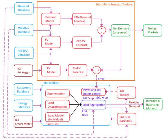
Figure 1.
Methodology flowchart.
A quantitative analysis for demand-side flexibility seems necessary thorough the definition and the evaluation of some indicators (i.e., DR indices in Figure 1) that allows to score the flexibility and performance of loads being controlled, basically at the aggregated level. These indicators converge with the idea of some voluntary schemes in the EU that intend to express the “readiness of a building” (in this case the readiness of the load inside buildings). According to these proposals [31], these indicators mean: “readiness to adapt in response to the needs of the occupants, readiness to facilitate maintenance and efficient operation, and readiness to adapt in response to the situation of the energy grid”. Taking into account this last requirement, a score is performed through the indicators to be described in Section 3.4.3.
2.2. Characteristics of the Customers: Demand, Photovoltaic Generation, and End-Uses
All electricity customers from a small town (4400 inhabitants), sited in the north Spain, have been selected for simulation purposes in this work. These customers include residential, commercial, and industrial clients, although most of the power consumption is due to the residential ones. Basically, this group corresponds to average residential customers in the south countries of the EU. The rated power per customer ranges from 3 to 8 kW. The climate is continental, and winter temperatures range from 0 to 13 °C and in summer from 13 to 29 °C.
Regional investors built a PV plant in the vicinity of the town, with a significant capacity with respect to its power demand. The PV plant is composed of two-axis solar trackers with a rated power of 1.9 MW, and it is connected to the same power substation that links the town to the grid.
Hourly load and photovoltaic generation data from 1 October 2008 to 31 March 2011 (both included) were available. These data were obtained from the electric utility distributor and corresponded to hourly average power measurements in the substation. It is worth mentioning that it has been very difficult to obtain real data corresponding to a considerable customer group that can act as prosumers (consumers and producers); thus, we had to manage data not as recent as desired.
Figure 2a shows the winter and summer loads for two selected workdays monitored at the distribution level (substation) that supplies power at 13.2 kV to the distribution transformer centers (CT) of customers (basically residential and commercial supply). Figure 2b shows the average temperature in the area for the same two selected workdays. Figure 2c plots the hourly PV power generation on the peak production days (days with the highest energy generation) of January and June 2010. The PV power generation values in the central hours of the day can mean an important fraction of the town consumption (30–40%). The selection of January and June as representative months is due to the fact that June corresponds to the month with the highest PV generation, while January corresponds to the lowest PV generation and the highest energy consumption. In Figure 2, it is also shown the average profiles of demand, temperature and PV generation for the period in which data is available (from 1 October 2008 to 31 March 2011). It is remarkable that the average PV generation profile (Figure 2c) is lower compared to the other ones (June and January). This fact can be explained because months’ profiles are representing the peak power days, while the average profile includes days in which there are no PV generation due to adverse weather conditions.
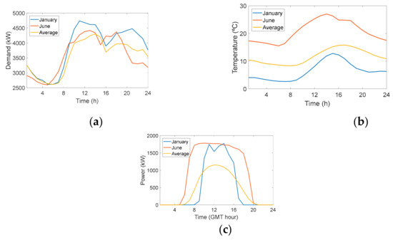
Figure 2.
Load, Temperature and PV Generation profiles: (a) example of winter and summer Load Curves in the power substation; (b) example of winter and summer temperature behavior; (c) example of winter and summer power generation in the PV plant on peak production days.
The use of DR portfolio for damping both the errors in the evaluation of demand in short-term and the intrinsic variability of PV generation sources need the evaluation of DR potential and its flexibility in each customer segment. First, this evaluation must be based on the knowledge of end-uses for an average customer. The first alternative to know demand composition behind-the-meter is the use of the information provided by Smart Meters (SM) and then apply some Non-Intrusive Load Monitoring (NILM) methodology, for example [32]. This last approach involves the full development of capacities of available home automation technologies, considering the increasing deployment of Smart Meter in several countries around the world [33]. Some of these methodologies have been reported by authors in previous papers [34] to obtain end-use disaggregation/profiles in residential segments and their real flexibility when DR policies are applied (i.e., DR validation).
In some cases, and from a practical point of view, it is possible that some problems arise for a practical implementation of DR based on end-uses, for instance: small customers do not have yet any SM, confidentiality of data is in question, Data Exchange Platforms (DEO) are not fully developed, and the availability of data is scarce [35] or the aggregator has access to meter data but without the necessary granularity or quality (i.e., it is usual to have data with granularity ranging from 15 min to 1 h which usually makes much more complex the identification of loads through NILM methods). In this way, an alternative access to demand data should also be considered by aggregators to accomplish the evaluation of DR potential. This alternative is based on periodic surveys performed by international or national Energy Agencies, for example EIA (data from 2015, [36]) in the United States or the Joint Research Centre (data from 2016, [37]) in the European Union. In this way, a residential “average” EU or USA customer (and its end-use share) can be estimated according to these data. In the case under study, available reports from the Institute for Energy Diversification and Energy Savings (IDAE, Spain) and the Spanish Government [38] have been analyzed. Table 1 depicts the main end-uses for Spain, EU-28 countries and the USA. Notice that in European Mediterranean countries, the Air Conditioning load represents a higher percent (66% of households have this appliance and the increasing trend is quite solid). A similar trend can be reported in the USA, because 87% of homes use air conditioning. It accounts for 12% of annual residential energy expenditures and is a large factor in fluctuations in residential electricity use. Heat Pumps (HP) exhibit similar trends according to EIA estimations [36]: the share of heated homes using HP increased from 8% to 12% in a decade (from 2005 to 2015). At the same time, the share of homes using electricity for water heating (WH) increased by 7% (to 46%). Due to this fact, both loads (HP and WH) have been considered to evaluate demand flexibility in this work. Moreover, winter period has been selected for simulation purposes in the following paragraphs, because demand in winter is higher than in summer and the climate in this Spanish area is more restrictive for PV generation possibilities.

Table 1.
Main end-uses share in the residential sector according to some estimates in the USA [36], EU-28 [37], and Spain [38] adapted and updated from [39].
To obtain some representative profiles, it seems necessary to evaluate load dynamics, and the service the customer obtains from them. Figure 3a,b shows some real end-use load profiles for a household belonging to the overall customer demand, previously shown in Figure 2. In this case, feedback from everyday activities [40] of the customer is important to refine profiles, improve DR&EE (Demand Response and Energy Efficiency) success and gain customer interest in energy concerns. Regulations can help aggregators to establish load profiles. Figure 3a shows an average HP consumption profile in winter, as in this study, DR simulations to balance generation are focused on this period. Figure 3b shows an average water flow use to determine WH requirements extracted from EN 15316-3-1, Section 5 (EU normative). Figure 3c shows the proposed end-use profiles for an average customer.
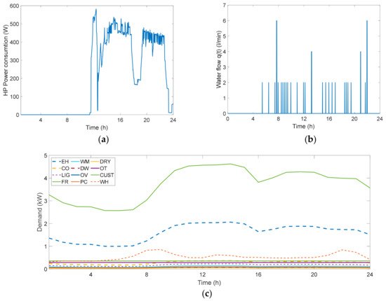
Figure 3.
Daily end-uses and customer service: (a) HP profile; (b) daily use of residential Water Heater. (c) Daily profiles for main end-uses (winter). Acronyms: EH: Heating (Electric heaters and Heat pumps), WH: Water Heating; CO: cooking; LIG: lighting; FR: fridges; WM: washing machines; DW: dishwasher; OV: Oven; PC: computers; DRY: dryers; OT: Others; and CUST: overall customer demand.
The procedure for obtaining end-uses profiles (Figure 3) could be explained as follows. In the first place, the aggregator needs to recover basic information about customer daily overall demand (aggregated or not) through Smart Metering (Figure 1, left bottom side). This information, alongside weather databases and public reports of energy household demand and share of end-uses in terms of energy, allows the aggregator the calculation of “household baselines”. At this point, the aggregator is able to run and refine Physically Based Load Models (PBLM) both at elemental and aggregated levels (i.e., include inputs/outputs for these models). With PBLM and average weather inputs the aggregator obtains “end-use baselines” for each end-use with relevant potential for DR (e.g., HVAC, space heater, WH, or thermal ceramic heaters, Figure 1), and their average daily demand in each season/month. Finally, “elemental baselines” (kWh and profiles) are modulated through coefficients (considering weather conditions and customer behavior) to fit the “overall baseline” for the customer.
2.3. Short-Term Forecasting Methods
In this section, the forecasting methods used to predict hourly load and PV generation are described.
2.3.1. Random Forest
Random forest is an ensemble method based on regression trees whose efficiency in load forecasting has been widely illustrated [15]. Being based on regression trees makes random forest a flexible method in case of complex and non-linear relationships, and as an ensemble method, it can provide low bias and reduces the variance of predictions.
Some other ensemble methods based on regression trees are bagging, conditional forest or boosting, whose efficiency in load forecasting has been shown in different papers (see for instance [41]).
Random forest is a generalization of bagging (bootstrap aggregating), but only a random sample of “mtry” predictors can be chosen at each split of the regression tree. This approach will reduce the variance of the estimations more than bagging, mainly in the case of correlated predictors. In this paper we have decided to use random forest to predict the electricity consumption instead of conditional forest of boosting due to its simplicity in parameter calibration and fast computation.
The efficiency of random forest depends on a suitable selection of the number of trees N and the number of predictors “mtry” tested at each split. However, random forests will not overfit when N increases, thus, we can focus on calibrating only the parameter “mtry”. The calibration of the parameter and the random forest method have been implemented throughout the R package “caret”, see [42].
2.3.2. Stochastic Gradient Boosting (SGB)
Another ensemble method based on regression trees is the stochastic gradient boosting. It has been successfully used in short-term load [43] and PV power [44] forecasting applications. The SGB method is based on the sequential construction of additive regression models, usually in the form or regression trees with a maximum tree size. At each iteration, the models are fitted, by least squares, to a random sample of pseudo-residuals of the previous stage. Thus, the SGB method applies a gradient descent algorithm, reducing the error (difference between output value and expected value) at each iteration.
The develop of an SGB forecasting model requires the selection of the values for a set of tuning parameters which include the number of trees (also called as iterations), the interaction depth, the shrinkage or learning rate, the minimum number of observations in terminal nodes of the trees, and the bagging or sampling fraction. Unlike the random forest method, SGB models with many trees are prone to overfitting; thus, that number must be carefully chosen. The complexity of the SGM model is related to the interaction depth which corresponds to the maximum size of each tree. The shrinkage parameter manages the influence of each sequential tree on the final value provided by the SGM model. The minimum number of observations in terminal nodes or leaves of the trees limits the observations used to provide their mean value as the response of that terminal node. Finally, the bagging fraction corresponds to the fraction of the training dataset observations randomly selected to build each tree (small values reduce the possibility of overfitting, but increase the model uncertainty). For a detailed description of the SGB method, see [45].
2.4. Time-Series Clustering
Clustering is an unsupervised technique whose objective is to separate objects (represented by a multivariate dataset) into homogeneous groups (called clusters), such that objects in the same cluster have high similarity among them, but low similarity with the objects in a different cluster. It is considered an exploratory technique very useful by itself or as a previous step for other kind of data analysis. Depending on the way the clusters are generated, clustering methods can be divided in two big sets: hierarchical methods and divisive methods. In addition, the resulting clusters are determined by the distance or similarity measure and the linkage method selected.
A special case is time-series clustering, where each object to be grouped corresponds to a sequence of values as a function of time. One of the main advantages of clustering time-series is that it allows the discovery of hidden patterns in time-series datasets. Generally, three different objectives can be considered in this context: finding similar time series in time, in shape, or in change (structural similarity). The selection of a suitable distance measure is essential and depends on the objective pursued. Interesting surveys in the field can be found in [46,47].
In this paper, we have focused on similarity in shape to cluster the daily curves of photovoltaic generation. Dynamic Time Warping (DTW) distance, described below, was chosen for that purpose. Regarding the nature of the clustering, hierarchical technique together with average linkage were selected. These clustering methods were developed by means of the R package TSclust [48].
DTW distance, introduced by [30], is commonly used for measuring shape-based similarity between two time series, which may vary in timing. The main advantage against other shape-based distances such as Euclidean or Wavelet Transform is its invariance to warping. In our context, daily curves of PV generation are conditioned by sunlight hours, which vary along the different seasons. That makes DTW distance suitable for clustering a set of daily PV curves along different years.
Given two time series (xi) I = 1, …,m and (yj) j = 1, …, m, it starts calculating a nxm matrix D = (Dij) with the distance between every possible pair of point xi and yj in the two time series, Dij = d(xi,yj), I = 1,…, n, j = 1, …, m, where d(xi,yj) can represents the Euclidean or the absolute distance. According to [30], a warping path w is a contiguous set of matrix elements which defines a mapping between (xi) and (yj) that satisfies the following conditions:
- Boundary conditions: w1 = (1; 1) and wk = (m; n), where k is the length of the warping path.
- Continuity: if wi = (a, b) then wi−1 = (a’, b’), where a − a’ ≤ 1 and b − b’ ≤ 1.
- Monotonicity: if wi = (a, b) then wi−1 = (a’, b’), where a − a’ ≥ 0 and b − b’ ≥ 0.
The objective in DTW distance is to find the shortest warping path. Due to its high computational cost, different approaches have been proposed to optimize the calculation (see [49]).
2.5. Demand Response Strategies
Demand Response policies have been used by ISOs since the early 1980s. In the first years of DR, the objective was to achieve a more rational planning and operation of resources. In recent years, with the development of energy markets and the increasing share of RES in the generation mix, DR becomes more centered in the customer and in the integration of the available RES potential. Demand Response can be divided into explicit and implicit DR. Implicit DR means the change of demand due to prices whereas explicit DR involves the change of demand when System or Distribution Operators (i.e., ISO or DSO) forecast and declare an event into the system in the short-term.
To respond to these events or prices, the most common policy is to limit demand. This reduction can be performed through the cycling of power supply (the supply is switched ON and OFF alternatively following a rectangular wave u(t)). If the natural “cycling” of the end-use being controlled, m(t) (the operating state of the control device), is greater than u(t), the DR action is effective (notice that an appliance can describe cycles or not, for example a fridge or an inverter heat pump, but every load has its operating state m(t) with respect to rated power). Considering that, in practice, demand measurements are discrete (every 5, 15 or 60 min) and it is necessary to define average values in a time period [t, t + k]. Mathematically, Equation (1):
where (t, t + k) and ū(t, t + k) are mean values of m(t) and u(t) in the time period k, respectively, and tON is the time in this period where a “representative” (average) load remains switched ON and demands power.
The models to be used (to obtain m(t) and apply u(t)) are PBLM, a methodology proposed first to solve problems such as cold load pickup. The main reason for this choice is that these models are “white” [50] or “grey” [51] models which allow physically explaining the dynamics of the appliance and its environment and consequently foreseeing its changes. In this work, PBLM “grey” models for HVAC (Heating, Ventilation and Air Conditioning) and WH loads (heating and ventilation) previously proposed in [39] have been used. Figure 4 shows an electrical-thermal equivalent for this model for heating loads (a broader explanation of parameters can be found in several references [52,53]).
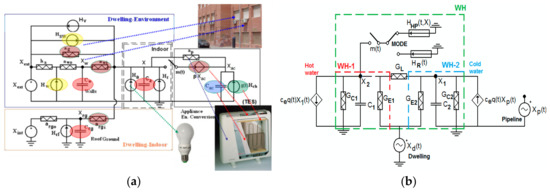
Figure 4.
Example of PBLM for: (a) HVAC (Heating, Ventilation and Air Conditioning); (b) WH (Water Heater).
The main features of these models are: they consider heat gains and losses, for instance solar radiation (Hsw, Hw) or internal gains due to inhabitants (Hr) or appliances (Ha) (Figure 4a); the model takes into account heat storage from the specific heat of external walls (Cw), indoor masses (Ca, C1 and C2, especially important for WH) or roof/ground (Crg); and it considers the control mechanisms which drive appliances (for instance thermostats m(t) and DR policies u(t)). Moreover, their state variables are temperatures: indoor (Xi), walls (Xw), roof/ground (Xrg) for HVAC loads (Figure 4a), and X1, X2 for the stratification of water in the reservoir (“hot” WH1 and “cold” WH2 sub-tanks, Figure 4b), that is to say, characteristics that allow the evaluation of energy flows and storage capabilities (i.e., the indirect capacity of storage in the envelope of buildings), the direct storage in WH or the loss of customer service due to the application of DR (i.e., internal or hot water temperature).
These models are individual ones and need a further aggregation to reach a minimum demand level (size of reduction packages) established by specific regulations of electricity markets to bid or offer into these markets (e.g., from 100 kW to 1 MW depending on each specific service or market [54,55]). This task is often developed by energy aggregators.
To achieve these packages, the aggregator needs to rise ON-time to increase demand of each specific end-load whereas a decrease of demand requires a reduction of ON-time. The second alternative (the traditional one) is easier because the aggregator only needs to manage the rate of switching-OFF and switching-ON times of the power supply to load. This is easy to perform through hardware by classical methods (e.g., ripple control of WH in Germany, [56,57]) or home automation methods (e.g., controlled plugs through Z-Wave protocols [58] and universal software platforms for control [59]).
An important concern for the practical implementation of modern DR policies is the Automated Demand Response (ADR), because customer manual control does not fit the requirements both of accuracy and reliability of response. It is imperative for the success of ADR the development of standards for the communications between operators, aggregators and their customers’ automation equipment [60] and the feedback from them. Open automated demand response protocol (OpenADR [61]) represents a good example of such a standard. Every day, more and more devices are certified to use OpenADR 2.0 protocols, and especially Smart Thermostats, but this certification is not necessary if some gateway assumes the role of “last-mile” controller and is compliant to receive and transmit OpenADR protocols. For example, home automation platforms such as Universal Devices ISY994 Series [62] allows the communication of residential customers with OpenADR, sending consigns and commands to home automation technologies working with different protocols (Zwave+, Insteon/X10, Zigbee Pro, Amazon Echo or Google Home). Other platforms, from well-known manufacturers, such as ABB SACE’s Emax 2 Power Controller, develop similar functions [63] but at building scale. Examples of ADR capabilities of grid-integrated buildings and building microgrids, architecture, and standards can be found in [60].
The rate of change is defined to the PBLM software by PWM waves: the carrier wave being tried has a frequency of 0.833 mHz (i.e., 1 cycle every 20 min) and the modulating waveform is the desired decrease in the average value in m(t, t + 20 min) according to deviations between 24-h PV forecasts (see Section 3.2) and 1-h PV forecasts used in markets (Figure 1).
The reasons for choosing 20 min have physical and technical senses. The first can be explained from the point of view of load service in the case of HVAC: if a harsh control is needed, switch-OFF times greater than 20 min can cause thermal fluctuations in the dwellings, easily noticeable by consumers (this can produce a lack of customer engagement in DR). The second reason is the so-called “lock-out” or mechanical delay of heating and air conditioning units. This mechanism is used to prevent a rapid recycling of the compressor avoiding mechanical damages. From the point of view of DR, it can cause an additional delay when applying ON/OFF and thermostat control signals. To evaluate the effect and characterize (from a statistical point of view) this process, some residential HP appliances (rated power from 1 kW to 3 kW) were monitored by authors. Changes in customer demand due to control actions have been recorded by an electronic meter and several Z-wave wall plug switches which send data to PCs using an USB gateway. Results depict that ON latency time ranges from 20–60 s and OFF latency times range from 10–40 s [64]. That is to say, the minimum ON-time should be in the range of one minute to limit inherent errors due to latency.
The first alternative (i.e., the increase of demand) is a less traditional option for DR [65]. Several reasons explain both the lack of use of these alternatives and their real interest. For instance, the increase of demand requires the control of thermostats. This control is more expensive than the supply control because smart thermostats are expensive. The cheapest option (e.g., Z-Wave) cost around € 150–200, whereas a remote switch costs around € 40–60. Fortunately, modern appliances include control of temperature though mobile-phones or PC, and these alternatives can be used for control (notice that some of them are compliant with well-known DR standard protocols [61]). In other cases, where the control device is intrusive (this is the case of WH), the cost of thermostat is similar, but the same maintenance (labor cost) is needed to include this option in the appliance. Over the last few years, some HPWH manufacturers in the USA have included these options for large units (200–500 L reservoir/storage tanks), for example [66].
The control of the thermostat (up or down, according to season, and usually used for pre-heating or pre-cooling policies in the dwelling being conditioned) has been proposed as a “virtual-storage” resource [67] for customers to take profit from Time of Use (ToU) tariffs or to “prepare” loads to face to DR events policies and maintain customer service (i.e., internal temperatures of houses or dwellings).
Usually, these policies have been used before the load is controlled, but the proposal in this paper is to use them continuously to adapt demand to changes in the forecasted PV generation. The control of the thermostat is evaluated and changed, if necessary, ±0.5 °C every 20 min. The reason for selecting this value is that 0.5 °C is a usual value for the change of temperature settings in home smart-thermostats.
In this way, the proposed control strategy u(t, t + k) for heating is done by Equation (2):
where Xsup is the upper temperature of load’s thermostat, which is set as a simple hysteresis cycle with dead-band db (usually ranging from 0.01–0.03 pu), and Xlim is the maximum reasonable temperature inside the dwelling (for example 22–23 °C in the case of HVAC, in winter) or the maximum temperature of water inside the tank (68 °C), which avoids risk of burns if a mixing valve is not used for the control of hot water pipeline. Xiserv is a minimum service level for the appliance (a minimum comfort temperature inside the dwelling, for example 16 °C, or a minimum temperature of hot water inside the WH, for example 36 °C).
Basically, Equation (2) means that load control is done by a double control. In the case of heating (electric heaters or HP) if the load must go up, the thermostat goes up until it reaches the maximum allowable value (Xlim). Otherwise, if demand must fall to balance a decrease in PV generation (with respect to 24 h forecast), the thermostat or the supply is controlled to reduce demand. Notice that a “baseline”, (i.e., load demand evaluated without control m(t, t + k)) is also needed as reference for controlled load. This baseline also comes from PBLM models (Figure 1).
3. Results and Discussion
3.1. Prediction Results for the Electricity Consumption
In this subsection, we provide 24-h-ahead predictions for the electricity consumption of the Spanish town in order to apply them to the context of Demand Response. For that, the ensemble method random forest described above was applied and some other aspects such as predictors importance or parameter selection was also developed.
On the one hand, it is well known that hourly loads of the previous days are the most important factors in short-term load forecasting. On the other hand, temperature is a factor that might affect the electricity consumption (cooling and heating of buildings). Therefore, prediction of hourly temperature for the location of the town under study was also used as an input in the load forecasting model, obtained as explained in the Section 3.2. In addition, several calendar variables such as the hour of the day, the day of the week, the month of the year and holidays have been taken into account in the design of the load forecasting model. Table 2 depicts the 49 predictors used for the load forecasting model: 23 dummies for the hour of the day, six dummies for the day of the week, 11 dummies for the month of the year, one dummy for holidays, one predictor of the forecasting temperature and seven predictors of historic loads (lags 24 h, 48 h, 72 h, 96 h, 120 h, 144 h, and 168 h).
Table 2.
Description of the predictors.
Before any analysis, a previous data filtering has been developed in order to detect and substitute missing cases or measurement errors. Moreover, in all cases the training period for model fitting ranges from 1 October 2008 to 31 November 2010, whereas the test period ranges from 1 January 2011 to 31 March 2011.
Three different measurements, given in Equations (3)–(5), were used to obtain the accuracy of the forecasting models: the root mean square error (RMSE), the R-squared (percentage of the variability explained by the forecasting model), and the mean absolute percentage error (MAPE).
The root mean square error is defined by:
The R-squared is given by:
The mean absolute percentage error is defined by:
where is the number of data, is the actual load at time , is the forecasting load at time , and is the mean value of the actual load. A slightly variants of this measure are the mean absolute error (MAE) and the cumulative absolute error (CAE).
Taking into account that the accuracy for special days (weekends and holidays) is usually lower than for regular days, the above goodness-of-fit measurements were obtained separately for each group of the test data.
Parameter tuning in random forest mainly refers to select an optimal number of trees (ntree) and an optimal number of predictors considered at each split (mtry). In fact, the selection of parameter ntree is quite easy because higher values do not lead to overfitting; thus, only a high enough value is needed. The optimal mtry = 12 was obtained by means of 10-fold cross-validation with three repeats and using a random grid with nine values (among the 49 possible).
Table 3 shows the goodness-of-fit measures for the training and test datasets after applying random forest with ntree = 200 and mtry = 12, and even for regular and special days separately. Furthermore, the importance of each predictor in the forecasting model has been obtained through the node impurity, getting that the electricity consumption at the same hour of the previous week (predictor LOAD_lag_168) is the most important predictor and that the following five most important ones are also historical loads. Temperature was in the 11th position of importance.
Table 3.
Goodness-of-fit measures for regular and special days in the training and test datasets.
Figure 5 represents the evolution of the goodness-of-fit measures for each hour of the day, where the best accuracy is reached early in the morning.
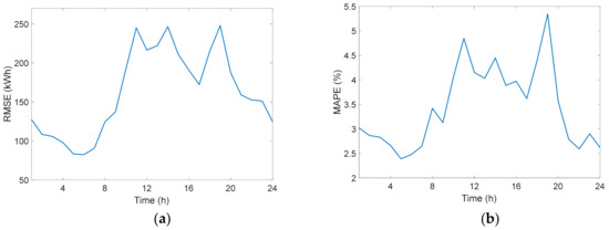
Figure 5.
Goodness-of-fit measures by hour of the day in the test dataset: (a) using RMSE; (b) using MAPE.
As an example, Figure 6 shows the actual and predicted load for a complete week in the test dataset.
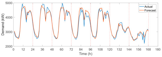
Figure 6.
Actual and forecasting load for a week (14–20 February 2011).
3.2. Prediction Results for the Photovoltaic Generation
In this subsection, we describe the short-term PV power forecasting model able to offer 24-h-ahead predictions for the PV plant placed in the town under study in the context of Demand Response. As mentioned above, this forecasting model is based on the SGB method, which allowed the creation of the forecasting model with the lowest RMSE from a set of models developed with techniques such as linear multivariate regression, artificial neural networks, random forest, and support vector machines. The SGB method was selected because it achieved the lowest RMSE with a five-fold cross-validation procedure with the training dataset. All the forecasting models used the same training dataset, and their parameters were optimized following a similar procedure to the described, for the SGB, in the following paragraphs.
Table 4 shows the explanatory variables used to develop the PV power forecasting model. The dependent or output variable was the hourly power generation in the PV plant for each hour of the day (only daylight hours were considered). The explanatory variables include hourly weather predictions obtained with the Weather and Research Forecast (WRF) mesoscale model [68], a numerical weather prediction (NWP) model able to produce forecasts for a geographical region with the desired spatiotemporal resolution. In order to produce the weather forecasts, the WRF model is started every day with the initial and boundary conditions provided by the forecasts of the GFS model, an NWP model with global coverage, run and maintained by the National Centers for Environmental Prediction (NCEP) from USA. From the values provided by the GFS model with a 1° × 1° (latitude–longitude) spatial resolution for the 00:00 Universal Time Coordinated (UTC) cycle, the WRF model provided predictions of weather variables over the region where the town under study is located with a time resolution of one hour, and a spatial resolution (distance between points of the grid of analysis) around 12 km. The forecasts of the desired weather variables for the location of the PV plant, or for the location of the town, were calculated by bilinear interpolation from the forecasts for the four nearest grid points. For a real operation, these weather predictions can be available for a new day before dawn and include all the forecasts for the 24 h ahead.
Table 4.
Explanatory variables for the PV power forecasting model.
The WRF model provided the hourly values of most of the 17 explanatory variables of Table 4 (variables from swflx to clear). The variable swflx corresponded to the global horizontal irradiance. Wind speed and direction were included because of the effect they could have on the temperature of the PV panels and, therefore, in their efficiency. The aghi variable matched to the average value of the forecasts for two consecutive hours of the swflx variable, that is, the average value of the global horizontal irradiance throughout the last hour. The aip variable corresponded to the average value of the irradiance on the PV panel throughout the last hour and it was calculated considering the characteristics of the PV panel with two-axis trackers and the solar geometry, as the aggregation of the direct normal and total diffuse irradiances on the tilted surface of the PV panels. The direct normal irradiance was obtained with the Erbs model [69] using the values of aghi and the total diffuse irradiance was calculated by means of the King model [70]. The variables h1 and h2 were used to code the hour (on UTC hour basis).
In order to select the best structure of the forecasting model, an optimization methodology was used based on the genetic algorithm (GA) with advanced generalization capabilities. This methodology is the GA-PARSIMONY [71], which allows the selection of parsimonious models. The main difference of this methodology with respect to the conventional GAs is a rearrange in the ranking of the individuals based on their complexities, so that individuals with less complexity (in this case, models with a less complex structure) are promoted to the best position of each generation. The promotion of less complex models with respect to the rest of individuals in the same generation with comparable fitness, allows the obtainment of models with improved generalization capability.
The GA-PARSIMONY methodology is implemented in the R package GAparsimony [72], which was the tool used to optimize the PV power forecasting models. In the case of the SGB model, the optimization process could choose the number of trees (in the range 20–250), the maximum interaction depth (range 3 to 8), the shrinkage value (range 0.001 to 0.25), and the minimum number of observations per terminal node (range 2 to 8), as well as select the input variables among those available (Table 4). The bagging fraction was fixed in 0.5. The fitness function corresponded to the negative value of the average RMSE obtained with five-fold cross-validation and three repeats with the training dataset. The complexity of the forecasting models evaluated in the optimization process was ten times the number of input variables used by the model plus the square of the maximum interaction depth. The number of individuals per generation was 50, the maximum number of generations 100, and the re-rank error value 0.1 (individuals with lower complexity and difference in the fitness value lower than the re-rank error were promoted to top positions in the ranking of each generation). The final model, achieved after the optimization process, used only 11 input variables (swflx, hr, pres, prec, mod, clear, cfm, temp, dir, cfl, and h2), had 182 trees, its maximum interaction depth was 6, its shrinkage value was 0.1197, and the number of minimum observations in a terminal node was 3. Table 5 shows the goodness-of-fit measures for the training and test datasets, where the RMSE, R-Squared and MAPE values are calculated using Equations (3)–(5), taking as the actual PV generation power at time t and the forecasted value for such hour. The high MAPE values are mainly due to very low actual PV generations in early and late daylight hours, when a small forecasting error can correspond to a very high absolute percentage error value.
Table 5.
Goodness-of-fit measures in the training and test datasets for the PV power forecasting model.
Figure 7 plots the actual and forecasted hourly PV power generation values for a week in the testing dataset. Notice that the forecast is carried out each day before dawn and, up to now, no correction is applied along the day.
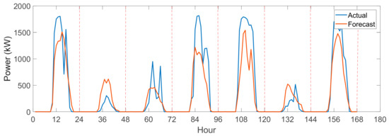
Figure 7.
Actual and forecasting PV power for a week (14–20 February 2011).
3.3. Classification Results of Photovoltaic Curves
The classification stage of the proposed method has been carried out in three steps: firstly, the predicted daily curves of PV generation corresponding to the training period (from 1 October 2008 to 31 December 2010) are clustered into homogenous groups using DTW distance and average linkage; secondly, the “desired” cluster is selected (the one whose predicted PV curves better fit the real PV curves) and a centroid curve for each resulting cluster is obtained; finally, each predicted daily curve in the test period (from 1 January 2011 to 31 March 2011) is classified into the nearest cluster by computing its DTW distance with each centroid curve. Those days in the test dataset of which the predicted PV curves are classified into the “desired” cluster will be the ones selected for applying DR policies.
First step described above implies the hierarchical clustering of 822 time series (number of days in the training dataset) of length 24 (hourly data). The resulting dendrogram provided five possible groups, whose centroid curves are given in Figure 8 (observe that the main difference among the curves falls on the magnitude of the generated energy, except for the fifth cluster). For each of the five resulting clusters, we computed the median of the percentage error for all days in the clusters, obtaining 19.36% for Cluster 1, 39.95% for Cluster 2, 77.41% for Cluster 3, 57.09% for Cluster 4, and 48.15% for Cluster 5. Therefore, Cluster 1 provided lower fitting errors than the rest of clusters, and hence, it was considered the “desired” cluster for our purpose. As the desired cluster provides lower errors, those forecasting PV curves of the test dataset that are classified into the desired cluster are expected to better fit the real PV curves than the ones that are classified into any of the not desired clusters.
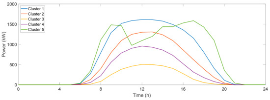
Figure 8.
PV centroid curves of each cluster in the training dataset.
The results obtained in the final step of the classification stage were the following. A total of 31 days in the test period were classified into Cluster 1 (the “desired” cluster), whose dates are given in Table 6 (recall that all days refer to year 2011) and some examples comparing the real PV and predicted PV (24 h ahead) are given in Figure 9.
Table 6.
Dates of the test period (2011) classified into Cluster 1 (and therefore selected for DR actions).
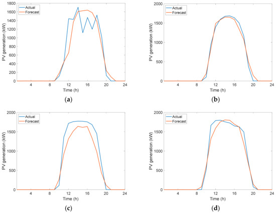
Figure 9.
Comparisons of actual PV and 24 h forecast PV generation for some days in Cluster 1: (a) day 3; (b) day 4; (c) day 9; (b) day 28.
3.4. Results for Demand Response Strategies
3.4.1. Very Short-Term PV Adjusted Forecasting
As was seen in Section 3.1 and Section 3.2, the main accuracy problem when obtaining a 24 h-ahead forecast of net demand is due to errors in the prediction of PV generation (compares Figure 6 and Figure 7), because this forecast is carried out each day before dawn, and no correction is applied during the day. The problem of balancing net load with respect to 24 h predictions should be taken into account by aggregators, because any imbalance can produce an important money flow from aggregators to Balance Service Providers (BSP) or Load Serving Entities (LSE). For this reason, a very short-term correction has been proposed. The idea is similar to the procedure used by ISOs to correct demand when some power event is declared in the system taking into account measurements of demand before the correction (i.e., the generation of customer’s baselines or CBL, for example [73]). In these methods (used for the retribution of demand response in reliability programs), the adjustment factor is obtained by means of the first two hours of the four-hour period prior to the commencement of the reliability event. In our case, the methodology to correct the forecasting values should balance accuracy and fast computation (it takes less than a minute to have enough time for the load control processing). In this stage, we propose the determination of an adjustment factor by means of the first 60 min of actual PV records of the one-and-a-half-hour period prior to the forecast window (it is assumed that PV generation has an SM able to record every minute and that sends this information to the aggregator). This adjustment factor is evaluated through the Equation (6):
where af(d, t) denotes the adjusted factor for the time t of the current day d used to fix generation forecasts, PVA(d, t − k) is the actual PV generation k min before, and PVF(d, t − k) is the predicted 24 h PV generation for day d at time t–k. Then, a first approximation of the forecasted PV baseline (PVBL_aux) is computed in the time interval [t − 30, t] to obtain [t, t + 30] values (that is, predictions are corrected in a time-window corresponding to very short-term according to the reduction of imbalances. For the participation of customers in other markets, the window can be enlarged according to gate closure times) through Equation (7):
To improve the goodness of this 1 h-ahead forecast, PVBL is compared with the average of historical values of PV generation in the last two weeks:
where PVupl is the upper limit considered as acceptable for any correction through the adjusted factor af(d, t). Therefore, Equation (7) is improved by Equation (9):
Results showed that the proposed correction by Equation (9) suits well its objective (Table 7 depicts the MAPE of the 24 h-ahead forecasts (PVF) and the 1 h-ahead forecasts (PVBL) for some representative days in Cluster 1). As expected, 1 h-ahead forecasts outperform 24 h-ahead forecasts, but achieve a significant improvement on days when the most serious errors took place (days 14, 16, 17, and 23). In some cases, a small increase of errors is reported (days 5 and 26).
Table 7.
Improvement in PV forecast attributable to the adjustment given in Equation (9).
3.4.2. Balancing Net Demand through DR
Once the predictions (for customers’ demand and PV generation) were calculated, and the clustering process selected the “desired” days for applying DR, the next objective was trying to adapt the net demand (difference between customers’ real demand and real PV generation) to the predicted net demand made for the day ahead (Figure 1).
In order to achieve this aim, DR policies were applied to two flexible loads: WHs and HVACs. The reason of choosing these loads is their facility for implementing control strategies by changing the thermostat temperature and their ability to act as thermal energy storage systems (by doing preheating of water in the case of WH and precooling and preheating of rooms/walls in the case of HVAC), see Section 2.5. DR policies were applied through PBLM and aggregation models [52], with the aim of ensuring that the final net consumption is adapted in a significant extent to the profile of net energy demand predicted the day before, so that it was not necessary to trade additional resources into the wholesale electricity market or to pay BSP.
The planning of DR actions that have to be performed was obtained hour-by-hour. That is to say that DR actions for each next hour were planned, taking into account the differences between predictions made for 24 h ahead and predictions made for 1 h ahead. As forecasts for electricity consumption are more accurate than PV forecasts, in this study, the predictions made for 1 h ahead only estimated the PV generation, thus, DR strategies only acted in order to manage the PV forecasting error. This fact means that the control was performed in the period in which there was PV generation, that is, approximately, from 8 a.m. to 9 p.m.
The PV variations between 24-h predictions and 1-h predictions must be compensated with changes in the consumption of WHs and HVACs. As WHs and HVACs represent the 17.9% and 42.9% of the total consumption, respectively (see Table 1); 25% of the PV variations was managed by WHs loads, and the rest (75%) was assigned to HVACs.
To demonstrate the ability of the loads (HVAC and WH) to adapt their consumption and the capacity of minimizing variability between predictions and real consumption and generation, the 31 days obtained from the “desired” cluster of PV curves have been simulated. Two different examples (days 14 and 23) have been selected to illustrate the application of DR strategies and its results, being explained in detail. Later, in Table 8 and Table 9, overall results and indicators for a set of representative days in Cluster 1 will be shown.
Table 8.
Results for the net energy consumption (day 23).
Table 9.
Results for net energy consumption (day 14).
Figure 10a,b presents the results for day 23 (21 March 2011) in which the PV generation forecasts made 24 h in advanced overestimate the real PV energy generated. As can be seen in Figure 10a, the forecasts made 1 h in advance are much more accurate; thus, they can be used as a baseline curve to plan the DR actions (Table 7 presents overall results). Figure 10b shows the effects on the net consumption forecasts. In order not to trade additional resources, the objective is to reduce the consumption in the way that the final actual net consumption matches the 24-h-ahead forecasts.
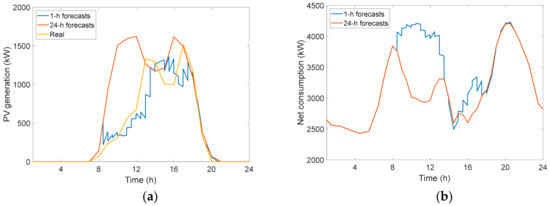
Figure 10.
Differences between 24-h-ahead and 1-h-ahead forecasts (day 23): (a) PV generation; (b) Net consumption.
Taking into account that there is PV generation only from 8 a.m. to 9 p.m., control actions will be applied to WH and HVAC only during this period. Figure 11 presents the variations in each predicted load demand that have to be performed to obtain the desired net consumption profile.
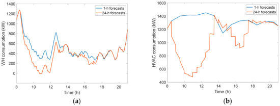
Figure 11.
Load demand variations between 24-h and 1-h forecasts (day 23): (a) WH; (b) HVAC.
Figure 12 depicts the load consumption after DR control strategies and the desired consumption profile from 24-h forecasts. As can be seen, DR actions work properly and the differences between the final and the “desired” load consumption have been significantly reduced.
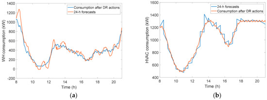
Figure 12.
Load consumption after DR actions and 24-h forecasts (day 23): (a) WH; (b) HVAC.
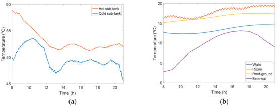
By modifying the WH and HVAC load consumption, it is also changed the temperature of water and rooms respectively. These variations can cause some comfort problems for users, thus, aggregators should assure that there are no large temperature variations and that the customer comfort is always guaranteed. This effect is considered in double control strategies defined in Section 2.5. by Equation (2).
Figure 13 shows the temperature profile of the loads. In the case of WHs (Figure 13a), the temperature is always above 45 and 50 °C in the cold and hot sub-tank, respectively [74]. Figure 13b shows the temperature of the rooms, the temperature of the internal walls, the temperature of the external walls, and the external ambient temperature. As can be seen, the internal temperature was always above 16 °C, while the maximum internal and ambient temperature (external) were 19.5 and 13 °C, respectively; the difference between internal and external temperature was always above 5.5 °C.
Finally, Figure 14 shows the net profiles for the 24-h-ahead forecasts compared with final net consumption after DR actions and the real net consumption if no DR action was performed.
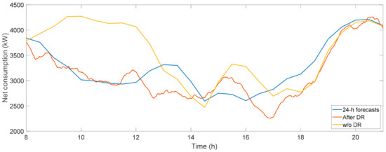
Figure 14.
Net consumption profiles (day 23): 24-h forecasts, after DR actions and without DR.
It is clearly demonstrated that DR actions significantly reduce the differences with 24-h-ahead net profile, efficiently compensating the forecasting errors and balancing the final net load consumption. Table 8 presents some numerical results from this example. All variables were calculated during the control period (from 8 a.m. to 9 p.m.).
As can be deduced from the Table 8, the total net consumption of the day is reduced from 45.96 MWh if no DR action is taken to 40.37 MWh if DR actions are applied. The differences between the 24-h-ahead forecasts and the final net consumption are also shortened: cumulative absolute error (CAE) reduces from 6.02 MWh without applying DR to 2.96 MWh with DR actions. In the same way, the percentage of error, understood as the rate between the CAE and the net consumption for 24-h-ahead forecasts, decreased from 14.27% (without DR) to 7.02% (with DR), which is a 51% of reduction.
In the next paragraphs, a different example of the DR strategy will be presented. In this case, day 14 (14 January 2011) was analyzed, where the 24-h-ahead forecast predicted less PV energy than the final real PV generation; thus, the aggregator has bought more energy than is necessary in Electricity Markets required. In order to not waste this energy, it was used to increase the temperature of WH and HVAC, exploiting their capacities to act as thermal energy storage systems. Figure 15a presents the 24-h-ahead and 1-h-ahead forecasts compared with real PV generation data. As can be seen, the 24-h-ahead forecasts have underestimated the PV generation, while 1-h-ahead forecasts have much more precision. Figure 15b shows that it is necessary to increase the final net demand to adapt the 1-h-ahead profile to 24-h-ahead forecasts, and in this way, consume the “excess” of PV generation.
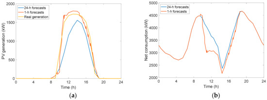
Figure 15.
Differences between 24-h-ahead and 1-h-ahead forecasts (day 14): (a) PV generation; (b) Net consumption.
Figure 16 depicts the results from the application of DR policies to the flexible loads (WH and HVAC). In both cases, the consumption after DR actions follow the target, to match its energy consumption with the 24-h-ahead predicted energy consumption for each load. Thus, it is fair to say that the DR control was working efficiently.
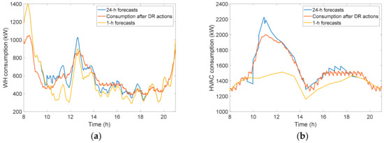
Figure 16.
Load demand variations among 24-h forecast, 1-h forecasts and final load consumption after DR (day 14): (a) WH; (b) HVAC.
As mentioned before, the increase in the energy consumption of both WH and HVAC was used to rise the temperature of the water inside the tank (in the case of WHs) and the temperature inside the rooms (HVAC). In the case of the WHs (Figure 17a), the temperature increases in the cold sub-tank from 49 to 59 °C and in the hot sub-tank from 58 to 63 °C (always ensuring that, for health security issues, the temperature is not above 68 °C in any WH), while in the HVACs (Figure 17b), the internal temperature of the rooms increased from 17 to 20.5 °C, whereas the maximum ambient temperature (external) was 11.5 °C.
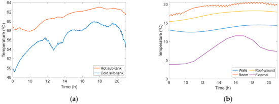
Figure 18 depicts the 24-h-ahead forecasts for the net energy consumption. The final net energy consumption profile after the application of DR strategies is also shown, as is its comparison with the net energy that will be consumed if no DR action is taken. The graph shows that DR actions reduced the differences between the 24-h forecasts and final net consumption, minimizing the necessity of selling back to Electricity Markets the PV generation surplus or to pay additional charges (or penalties) for unbalance in markets.
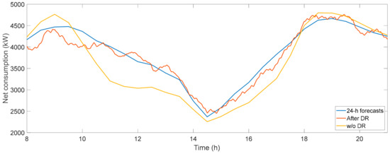
Figure 18.
Net consumption profiles (day 14): 24-h forecasts, after DR actions and without DR.
Table 9 presents some numerical results from this example. All variables were calculated only during the control period (8 a.m.–9 p.m.). Results show that the net energy consumption with DR strategies increased to 49.43 MWh compared with the 47.23 MWh consumed without the application of DR, and reached 50.13 MWh for 24-h forecasts. The variations between forecasts and final net consumption were reduced from 4.13 MWh to 1.79 MWh, reducing the percentage of error by 57% (from 8.25 to 3.58%). The maximum power peak difference was also reduced by 44%.
Table 10 shows overall results for net energy consumption of a representative part of the 31 days in Cluster 1. Day 16 (Figure 19a) obtained the greatest reduction in the error (from 31.63 to 6.7%), whereas day 28 (Figure 19b) was the one in which the percentage of error increased most (from 6.55 to 9.99%). Notice that this rise in the error was not due to DR actions, but because of the lack of accuracy in the prediction of customers’ load profile of that day (day 28), because only deviations of PV generations were corrected by means of DR (see also Figure 9).
Table 10.
Values for net energy consumption.
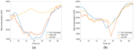
Figure 19.
Net consumption profiles: 24-h forecasts, after DR and without DR: (a) day 16; (b) day 28.
Finally, Figure 20 presents the cumulative absolute error for the 31 days in Cluster 1 when comparing the target (the 24-h-ahead forecast) with the final net consumption in two different scenarios (without DR and after DR actions). It can be seen that, in general, errors were reduced after DR, except in some particular days where they increased slightly. Notice that the set of days selected in Table 10 and Table 11 (among the 31 days belonging to Cluster 1) represent different scenarios (low, medium, and high reduction of the errors as well as increasing of them after DR policies).
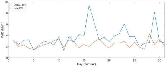
Figure 20.
Cumulative absolute error (CAE) between the final net consumption (without DR and after DR actions) and the target (the 24 h-ahead forecast of the net consumption).
Table 11.
DR performance and flexibility indicators.
3.4.3. Analysis of DR Flexibility
As mentioned in Section 2.1, a quantitative analysis for demand-side flexibility has been performed thorough some indicators defined and calculated at an aggregated level.
The first indicator of flexibility refers to signals’ dynamic. This is done through an indicator that gives an idea about the variation of a signal and it is very close to the “mileage” score used for the verification of assets in Ancillary Services. In this way, the “signal_mileage” is the absolute sum of movement of the analyzed signal in a given time period with respect to the average value of the signal, in our case daily:
where signal refers to the target foreseen for balancing PV generation through load (variable “balance”) or the load demand (with DR or without DR, i.e., the variable “baseline” of demand or the new demand with DR, in this case the variable “demand_DR”). These indicators give, respectively, an idea of the variability of demand (hourly, daily,...) for the segment under study and the “amount of work” involved through “balance” signals to match PV/demand forecast errors.
A second indicator is the “mileage_ratio”, which measures the relation of the value of mileage of the balance signal sent to flexible demand versus the value of changes in demand in the steady state (without DR). This indicator gives the aggregator a first insight with respect the effort that demand is forced to yield to match PV generation in the short-term:
The third indicator represents the symmetry of the effort required from demand to follow the energy balance signal (i.e., the overall increase of flexible demand versus the reduction of demand). As has been discussed in previous paragraphs, in some cases, it is more difficult for the load to increase in demand than achieve a reduction in demand (for instance, electric heating in winter). For these reasons, the positive changes in demand were evaluated with respect to negative changes of demand. Mathematically:
Finally, the aggregator calculated a daily performance score that reflects the load resource’s accuracy in increasing or decreasing its demand to provide balance in response to balance dispatch signal. The performance score calculation evaluates each resource’s accuracy in following the balance signal, that is to say:
These indicators have been evaluated through and Table 11 presents the main results.
A brief explanation of the results can help the reader to better understand the physical meaning of these indicators. It is also interesting to consider the results of Section 3.4.2 for days 14 and 23. Table 11 shows that the days 14 and 23 require a noticeable effort from flexible demand (3.12 and 4.14 for “balance_mileage” values that are above the average effort). Steady state fluctuations of demand are similar for both days (5.72 and 5.28, see demand mileage column). This index (mileage_demand) is of interest to reflect unusual changes of demand pattern.
Column five in Table 11 presents the symmetry of the effort. Day 14 requires a net increase of demand (symmetry = 7.06), whereas day 23 basically requires a strong shaving of demand (symmetry = 0.038). The score for the performance of flexible demand depicts that flexible loads follow with enough accuracy their targets (performance indicator is around zero). Moreover, from Table 11, the aggregator can deduce that flexible demand fails in days 5 and 28 (performance has the greatest values and over 1), but these days do not represent a big problem, because the effort required from demand (balance_mileage) is low (1.52 and 2.08). These results and the results previously discussed in Section 3.4.2 help both the customer and the aggregator to familiarize themselves with the demand response and the usefulness of short-term predictions to manage their new role as prosumers or energy aggregators.
4. Conclusions
Energy issues are a main concern for the sustainability of our society. This sustainability is based on the integration of renewable sources and in the development of new energy markets, which should be more customer-centered than in the past. These objectives need the development and validation of additional tools to facilitate this change and to contribute to the effective engagement of customers in these markets, as has happened in telecommunications markets. Technological aspects, such as the forecast of demand and renewable sources or the management of energy, appeared as significant barriers to the effective deployment of new markets in small and medium customer segments, i.e., benefits usually do not balance the complexity for new responsibilities and tasks in these scenarios. Moreover, forecasts get more complex when the level of assets’ aggregation decreases, and this makes the above-mentioned objectives more difficult. For these reasons, this work developed and validated both demand and renewable generation forecasting methods at low aggregation levels (in the order of some MW) of the power system (distribution), but focused the methodological effort on the application of these methods to demonstrate the possibility of participation of “prosumers” in markets rather than in the achievement of small improvements in forecasts accuracy (MAPE, RMSE, CAE) through exponential complexity.
The interaction of demand, generation and management models demonstrated that this feedback or linkage among models can balance errors through a “closed control loop” that drove the net demand of “prosumers”. In the analyzed scenarios, results showed that 50% of prediction errors can be balanced with naïf correction models (very short term) and a “reduced” portfolio of loads (HVAC and WH) and policies. The paper also demonstrated the ability of these small and medium customers, through demand aggregators, to exhibit in the market the necessary flexibility in demand (up and down) to manage the volatility of renewables and build new power systems and new markets in the horizon 2030–2050.
Further developments are necessary to advance in this approach, for instance: the consideration of the participation of customers in new markets and more complex services (mixed participation in two or more markets or services), the refinement of very short-term models (both in demand and generation), the introduction and synthesis of new end-use PBLM and their further aggregation, the integration and deployment of ICTs in the models and the validation, the hybridization of ESS and demand models, both following PBLM philosophy, to provide more capabilities for flexibility, and the adjustment and improvement of these models in actual customers through pilots. In the medium term, and with these tools, the potential flexibility of these small and medium customer segments could be exploited and used to balance the integration of renewable both in Smart Grids and in conventional Power Systems.
Author Contributions
L.A.F.-J., M.C.R.-A., A.G. (Antonio Guillamón) and A.G. (Antonio Gabaldón) conceived and designed the experiments and structure of the paper. A.G.-G. and A.G. (Antonio Gabaldón) programmed the algorithms and developed and wrote the part concerning HVAC and WH modeling, the technical evaluation of prosumers, and the simulation and evaluation of DR targets. M.C.R. and A.G. (Antonio Guillamón) managed the customer database of demand/end-uses and supervised some of the mathematic algorithms for short-term load models. L.A.F.-J. and A.F. managed PV generation database and defined and supervised the mathematic algorithms for short-term PV generation models. All authors have approved the final manuscript. All authors have read and agreed to the published version of the manuscript.
Funding
This work was supported by the supported by the AEI/10.13039/501100011033, (Ministerio de Ciencia, Innovacióna y Universidades, Spanish Government) under research projects ENE-2016-78509-C3-2-P, ENE-2016-78509-C3-3-P, RED2018-102618-T, and EU FEDER funds. The authors have also received funds from these grants for covering the costs to publish in open access.
Acknowledgments
This work was supported by the Ministerio de Economía, Industria y Competitividad (Spanish Government) under research projects ENE-2016-78509-C3-2-P, ENE-2016-78509-C3-3-P, RED2018-102618-T, the Ministerio de Educación (Spanish Government) under doctorate grant FPU17/02753, and the special support of EU FEDER funds.
Conflicts of Interest
The authors declare no conflict of interest.
References
- Catalão, J.P.S. Electric Power Systems: Advanced Forecasting Techniques and Optimal Generation Scheduling; CRC Press: Boca Raton, FL, USA, 2012. [Google Scholar]
- Hahn, H.; Meyer-Nieberg, S.; Pickl, S. Electric load forecasting methods: Tools for decision making. Eur. J. Oper. Res. 2009, 199, 902–907. [Google Scholar] [CrossRef]
- Antonanzas, J.; Osorio, N.; Escobar, R.; Urraca, R.; Martinez-de-Pison, F.J.; Antonanzas-Torres, F. Review of photovoltaic power forecasting. Sol. Energy 2016, 136, 78–111. [Google Scholar] [CrossRef]
- Alfares, H.K.; Nazeeruddin, M. Electric load forecasting: Literature survey and classification of methods. Int. J. Syst. Sci. 2002, 33, 23–34. [Google Scholar] [CrossRef]
- Yang, H.T.; Huang, C.M.; Huang, C.L. Identification of ARMAX model for short term load forecasting: An evolutionary programming approach. IEEE Trans. Power Syst. 1996, 11, 403–408. [Google Scholar] [CrossRef]
- Taylor, J.W.; de Menezes, L.M.; McSharry, P.E. A comparison of univariate methods for forecasting electricity demand up to a day ahead. Int. J. Forecast. 2006, 22, 1–16. [Google Scholar] [CrossRef]
- Massana, J.; Pous, C.; Burgas, L.; Melendez, J.; Colomer, J. Short-term load forecasting in a non-residential building contrasting models and attributes. Energy Build. 2015, 92, 322–330. [Google Scholar] [CrossRef]
- Bruhns, A.; Deurveilher, G.; Roy, J.S. A non-linear regression model for mid-term load forecasting and improvements in seasonality. In Proceedings of the 15th Power Systems Computation Conference, Liege, Belgium, 22–26 August 2005. [Google Scholar]
- Charytoniuk, W.; Chen, M.S. Nonparametric regression based short-term load forecasting. IEEE Trans. Power Syst. 1998, 13, 725–730. [Google Scholar] [CrossRef]
- Li, K.; Su, H.; Chu, J. Forecasting building energy consumption using neural networks and hybrid neuro-fuzzy system: A comparative study. Energy Build. 2011, 43, 2893–2899. [Google Scholar] [CrossRef]
- Liao, G.C.; Tsao, T.P. Application of a fuzzy neural network combined with a chaos genetic algorithm and simulated annealing to short-term load forecasting. IEEE Trans. Evol. Comput. 2006, 10, 330–340. [Google Scholar] [CrossRef]
- Tso, G.K.F.; Yau, K.K.W. Predicting electricity energy consumption: A comparison of regression analysis, decision tree and neural networks. Energy 2007, 32, 1761–1768. [Google Scholar] [CrossRef]
- Dong, Y.; Ma, X.; Ma, C.; Wang, J. Research and application of a hybrid forecasting model based on data decomposition for electrical load forecasting. Energies 2016, 9, 1050. [Google Scholar] [CrossRef]
- Chen, K.; Chen, K.; Wang, Q.; He, Z.; Hu, J.; He, J. Short-Term Load Forecasting with Deep Residual Networks. IEEE Trans. Smart Grid 2019, 10, 3943–3952. [Google Scholar] [CrossRef]
- Dudek, G. Short-term load forecasting using random forests. Adv. Intell. Syst. Comput. 2015, 323, 821–828. [Google Scholar] [CrossRef]
- Lin, Y.; Luo, H.; Wang, D.; Guo, H.; Zhu, K. An Ensemble Model Based on Machine Learning Methods and Data Preprocessing for Short-Term Electric Load Forecasting. Energies 2017, 10, 1186. [Google Scholar] [CrossRef]
- Niu, D.; Wang, Y.; Wu, D.D. Power load forecasting using support vector machine and ant colony optimization. Expert Syst. Appl. 2010, 37, 2531–2539. [Google Scholar] [CrossRef]
- Zhang, X.; Wang, J.; Zhang, K. Short-term electric load forecasting based on singular spectrum analysis and support vector machine optimized by Cuckoo search algorithm. Electr. Power Syst. Res. 2017, 146, 270–285. [Google Scholar] [CrossRef]
- Zhang, J.; Wei, Y.M.; Li, D.; Tan, Z.; Zhou, J. Short term electricity load forecasting using a hybrid model. Energy 2018, 158, 774–781. [Google Scholar] [CrossRef]
- Li, Y.; Su, Y.; Shu, L. An ARMAX model for forecasting the power output of a grid connected photovoltaic system. Renew. Energy 2014, 66, 78–89. [Google Scholar] [CrossRef]
- Li, Y.; He, Y.; Su, Y.; Shu, L. Forecasting the daily power output of a grid-connected photovoltaic system based on multivariate adaptive regression splines. Appl. Energy 2016, 180, 392–401. [Google Scholar] [CrossRef]
- Abdullah, N.A.; Abd Rahim, N.; Gan, C.K.; Nor Adzman, N. Forecasting Solar Power Using Hybrid Firefly and Particle Swarm Optimization (HFPSO) for Optimizing the Parameters in a Wavelet Transform-Adaptive Neuro Fuzzy Inference System (WT-ANFIS). Appl. Sci. 2019, 9, 3214. [Google Scholar] [CrossRef]
- Chu, Y.; Urquhart, B.; Gohari, S.M.I.; Pedro, H.T.C.; Kleissl, J.; Coimbra, C.F.M. Short-term reforecasting of power output from a 48 MWe solar PV plant. Sol. Energy 2015, 112, 68–77. [Google Scholar] [CrossRef]
- Galicia, A.; Talavera-Llames, R.; Troncoso, A.; Koprinska, I.; Martínez-Álvarez, F. Multi-step forecasting for big data time series based on ensemble learning. Knowl. Based Syst. 2019, 163, 830–841. [Google Scholar] [CrossRef]
- Antonanzas, J.; Pozo-Vázquez, D.; Fernandez-Jimenez, L.A.; Martinez-de-Pison, F.J. The value of day-ahead forecasting for photovoltaics in the Spanish electricity market. Sol. Energy 2017, 158, 140–146. [Google Scholar] [CrossRef]
- Ferlito, S.; Adinolfi, G.; Graditi, G. Comparative analysis of data-driven methods online and offline trained to the forecasting of grid-connected photovoltaic plant production. Appl. Energy 2017, 205, 116–129. [Google Scholar] [CrossRef]
- Australian Energy Market Commission Integrating Distributed Energy Resources for the Grid of the Future. Economic Regulatory Framework Review. Available online: https://www.aemc.gov.au/sites/default/files/2019-09/Final report-ENERFR 2019-EPR0068.PDF (accessed on 6 November 2019).
- Sánchez Jiménez, M. Regulatory Proposal for deployment of flexibility. In Proceedings of the India SMART GRIDS Week, New Delhi, India, 8–10 March 2017; p. 15. [Google Scholar]
- EURELECTRIC Designing Fair and Equitable Market Rules for Demand Response Aggregation. Available online: http://www.eurelectric.org (accessed on 4 September 2019).
- Bemdt, D.J.; Clifford, J. Using Dynamic Time Warping to find patterns in time series. In Proceedings of the KDD Workshop, Seattle, WA, USA, 31 July–1 August 1994; pp. 359–370. [Google Scholar]
- Smart Energy Europe. SmartEn White Paper: A Vision for Smart and Active Buildings. Available online: https://www.smarten.eu/wp-content/uploads/2019/07/FINAL-smartEn-white-paper-Smart-Buildings.pdf (accessed on 6 November 2019).
- Zeifman, M.; Roth, K. Nonintrusive appliance load monitoring: Review and outlook. IEEE Trans. Consum. Electron. 2011, 57, 76–84. [Google Scholar] [CrossRef]
- Federal Energy Regulatory Commission (FERC). Assessment of Demand Response and Advanced Metering: Staff Report. Available online: https://www.ferc.gov/legal/staff-reports/2016/DR-AM-Report2016.pdf (accessed on 14 June 2019).
- Gabaldón, A.; Molina, R.; Marín-Parra, A.; Valero-Verdú, S.; Álvarez, C. Residential end-uses disaggregation and demand response evaluation using integral transforms. J. Mod. Power Syst. Clean Energy 2017, 5, 91–104. [Google Scholar] [CrossRef]
- Jenssen, Å.; Borsche, T.; Wolst, J. Data Exchange in Electric Power Systems: European State of Play and Perspectives; THEMA Consulting: Oslo, Norway, 2017; ISBN 9788283680133. [Google Scholar]
- Residential Energy Consumption Survey (RECS)—Data—U.S. Energy Information Administration (EIA). Available online: https://www.eia.gov/consumption/residential/data/2015/ (accessed on 6 November 2019).
- Bertoldi, P.; López Lorente, J.; Labanca, N. Energy Consumption and Energy Efficiency Trends in the EU-28 2000–2014; Publication Office of the European Commission: Luxembourg, 2016. [Google Scholar]
- IDAE Consumo por usos y Energías del Sector Residencial (2010–2017). Available online: https://www.idae.es/estudios-informes-y-estadisticas (accessed on 6 November 2019).
- García-Garre, A.; Gabaldón, A.; Álvarez-Bel, C.; Ruiz-Abellón, M.; Guillamón, A. Integration of Demand Response and Photovoltaic Resources in Residential Segments. Sustainability 2018, 10, 3030. [Google Scholar] [CrossRef]
- Ellegård, K.; Palm, J. Visualizing energy consumption activities as a tool for making everyday life more sustainable. Appl. Energy 2011, 88, 1920–1926. [Google Scholar] [CrossRef]
- Del Carmen Ruiz-Abellón, M.; Gabaldón, A.; Guillamón, A. Load forecasting for a campus university using ensemble methods based on regression trees. Energies 2018, 11, 2038. [Google Scholar] [CrossRef]
- Caret R Package. Available online: https://cran.r-project.org/web/packages/caret/caret.pdf (accessed on 6 November 2019).
- Ben Taieb, S.; Hyndman, R.J. A gradient boosting approach to the Kaggle load forecasting competition. Int. J. Forecast. 2014, 30, 382–394. [Google Scholar] [CrossRef]
- Wang, J.; Li, P.; Ran, R.; Che, Y.; Zhou, Y. A Short-Term Photovoltaic Power Prediction Model Based on the Gradient Boost Decision Tree. Appl. Sci. 2018, 8, 689. [Google Scholar] [CrossRef]
- Friedman, J.H. Stochastic gradient boosting. Comput. Stat. Data Anal. 2002, 38, 367–378. [Google Scholar] [CrossRef]
- Warren Liao, T. Clustering of time series data—A survey. Pattern Recognit. 2005, 38, 1857–1874. [Google Scholar] [CrossRef]
- Aghabozorgi, S.; Seyed Shirkhorshidi, A.; Ying Wah, T. Time-series clustering—A decade review. Inf. Syst. 2015, 53, 16–38. [Google Scholar] [CrossRef]
- Montero, P.; Vilar, J.A. TSclust: An R package for time series clustering. J. Stat. Softw. 2014, 62, 1–43. [Google Scholar] [CrossRef]
- Dau, H.A.; Silva, D.F.; Petitjean, F.; Forestier, G.; Bagnall, A.; Mueen, A.; Keogh, E. Optimizing dynamic time warping’s window width for time series data mining applications. Data Min. Knowl. Discov. 2018, 32, 1074–1120. [Google Scholar] [CrossRef]
- Wilson, E.; Christensen, C. Heat Pump Water Heater Modeling in EnergyPlus. In Proceedings of the Building America Residential Energy Efficiency Stakeholder Meeting, Austin, TX, USA, 29 February–1 March 2012; pp. 1–36. [Google Scholar]
- Li, X.; Wen, J. Review of building energy modeling for control and operation. Renew. Sustain. Energy Rev. 2014, 37, 517–537. [Google Scholar] [CrossRef]
- Gabaldón, A.; Álvarez, C.; Ruiz-Abellón, M.; Guillamón, A.; Valero-Verdú, S.; Molina, R.; García-Garre, A. Integration of Methodologies for the Evaluation of Offer Curves in Energy and Capacity Markets through Energy Efficiency and Demand Response. Sustainability 2018, 10, 483. [Google Scholar] [CrossRef]
- Demand Response (DR) Web Page. Available online: http://www.demandresponse.eu/ (accessed on 14 June 2019).
- NYISO Emergency Demand Response Program Manual. Available online: https://www.nyiso.com/demand-response (accessed on 4 September 2019).
- NYISO Day-Ahead Demand Response Program Manual. Available online: http://online.fliphtml5.com/qzli/zqaf/#p=1 (accessed on 6 November 2019).
- PROLAN Ripple Control Receiver and Tone Frequency Receiver (HKV-RKV). Available online: https://www.prolan.hu/en/solutions/HKV-RKV (accessed on 6 November 2019).
- TenneT und Bayernwerk: Dezentrale Flexibilität aus Bayern für die Energiewende—TenneT. Available online: https://www.tennet.eu/de/news/news/tennet-und-bayernwerk-dezentrale-flexibilitaet-aus-bayern-fuer-die-energiewende/ (accessed on 6 November 2019).
- Wireless Smart Home and Home Automation | FIBARO. Available online: https://www.fibaro.com/en/ (accessed on 6 November 2019).
- Symcom. IP-Symcon Integrators. Automation Software. Available online: https://www.symcon.de/en/product/integrators/ (accessed on 6 November 2019).
- Samad, T.; Koch, E.; Stluka, P. Automated Demand Response for Smart Buildings and Microgrids: The State of the Practice and Research Challenges. Proc. IEEE 2016, 104, 726–744. [Google Scholar] [CrossRef]
- OpenADR Alliance. Available online: https://www.openadr.org/ (accessed on 2 December 2019).
- Universal Devices Web Page. Available online: https://www.universal-devices.com/ (accessed on 2 December 2019).
- Cui, T.; Carr, J.; Brissette, A.; Ragaini, E. Connecting the Last Mile: Demand Response in Smart Buildings. In Proceedings of the 8th International Conference on Sustainability in Energy and Buildings, SEB-16, Turin, Italy, 11–13 September 2016; Volume 111, pp. 720–729. [Google Scholar]
- Gabaldón, A.; Álvarez, C.; Moreno, J.I.; Matanza, J.; López, G.; Ruiz-Abellón, M.C.; Valero-Verdu, S. Evaluation of the performance of Aggregated Demand Response by the use of Load and Communication Technologies Models. In Proceedings of the EEDAL Conference, Irvine, CA, USA, 13–15 September 2017. [Google Scholar]
- Monitoring Analytics LLC. 2019 Quarterly State of the Market Report for PJM: January through September. Available online: https://www.monitoringanalytics.com/reports/PJM_State_of_the_Market/2019/2019q3-som-pjm.pdf (accessed on 2 December 2019).
- Steffes, P. The Path to Grid-Interactive Water Heating (GIWH), Opportunities & Challenges. Available online: https://www.peakload.org/assets/36thConf/PLMA Steffes Presentation 11-13-17.pdf (accessed on 6 November 2019).
- Lueken, R.; Hledik, R.; Chang, J. The Hidden Battery. Opportunities in Electric Water Heating. In Proceedings of the PLMA Grid Interactive Behind the Meter Storage Interest Group Meeting; The Brattle Group; NRECA; NRDC; PLMA: Boston, MA, USA, 2015. [Google Scholar]
- Skamarock, W.C.; Klemp, J.B.; Dudhia, J.; Gill, D.O.; Barker, D.M.; Duda, M.G.; Huang, X.-Y.; Wang, W.; Powers, J.G. A Description of the Advanced Research WRF Version 3 (No. NCAR/TN-475+STR). Available online: https://opensky.ucar.edu/islandora/object/technotes%3A500/datastream/PDF/view (accessed on 6 November 2019).
- Erbs, D.G.; Klein, S.A.; Duffie, J.A. Estimation of the diffuse radiation fraction for hourly, daily and monthly-average global radiation. Sol. Energy 1982, 28, 293–302. [Google Scholar] [CrossRef]
- Lave, M.; Hayes, W.; Pohl, A.; Hansen, C.W. Evaluation of global horizontal irradiance to plane-of-array irradiance models at locations across the United States. IEEE J. Photovolt. 2015, 5, 597–606. [Google Scholar] [CrossRef]
- Sanz-Garcia, A.; Fernandez-Ceniceros, J.; Antonanzas-Torres, F.; Pernia-Espinoza, A.V.; Martinez-De-Pison, F.J. GA-PARSIMONY: A GA-SVR approach with feature selection and parameter optimization to obtain parsimonious solutions for predicting temperature settings in a continuous annealing furnace. Appl. Soft Comput. J. 2015, 35, 13–28. [Google Scholar] [CrossRef]
- ‘GAparsimony’ R Package. Available online: https://cran.r-project.org/web/packages/GAparsimony/GAparsimony.pdf (accessed on 13 November 2019).
- Lake, C. PJM Empirical Analysis of Demand Response Baseline Methods. Available online: https://www.pjm.com/-/media/markets-ops/demand-response/pjm-analysis-of-dr-baseline-methods-full-report.ashx?la=en (accessed on 4 September 2019).
- Gabaldon, A.; Valero-Verdu, S.; Garcia-Garre, A.; Senabre, C.; Alvarez-Bel, C.; Lopez, M.; Penalvo, E.; Sanchez, E.P. A physically-based model of heat pump water heaters for demand respose policies: Evaluation and testing. In Proceedings of the 2018 International Conference on Smart Energy Systems and Technologies, Sevilla, Spain, 10–12 September 2018; pp. 1–6. [Google Scholar]


© 2019 by the authors. Licensee MDPI, Basel, Switzerland. This article is an open access article distributed under the terms and conditions of the Creative Commons Attribution (CC BY) license (http://creativecommons.org/licenses/by/4.0/).