Annual Variation in Energy Consumption of an Electric Vehicle Used for Commuting

Abstract

The energy consumption of an electric vehicle is primarily due to the traction subsystem and the comfort subsystem. For a regular trip, the traction energy can be relatively constant but the comfort energy has variation depending on seasonal temperatures. In order to plan the annual charging operation of an eco-campus, a simulation tool is developed for an accurate determination of the consumption of an electric vehicle throughout year. The developed model has been validated by comparison with experimental measurement of a real vehicle on a real driving cycle. Different commuting trips are analyzed over a complete year. For the considered city in France (Lille), the comfort energy consumption has an overconsumption up to 33% in winter due to heating, and only 15% in summer due to air conditioning. The urban commuting driving cycle is more affected by the comfort subsystem than extra-urban trips.

1. Introduction

Climate change is a critical challenge for humanity in the 21st century. In developed countries, the transport sector is the largest producer of greenhouse gases that cause climate change. Electrification of vehicles is a way to reduce pollutants emissions [1,2]. In fact, according to the International Energy Agency, limiting climate change to 2 °C is possible if 150 million electrified vehicles are on the road by 2030 [3]. Many cities want to replace conventional vehicles by electrified vehicles or ban thermal vehicles completely [4].

As an example, the University of Lille would convert its “Cité Scientifique” into an eco-campus without thermal vehicles [5]. As this campus receives 22,000 daily users in 80 buildings, it is functionally a small city. Currently, mobility constitutes more than 50% of the greenhouse gas emissions of this campus. The CUMIN (Campus of University with Mobility based on Innovation and carbon Neutral) program [5] aims to reduce the emissions from thermal cars, using several strategies including replacing conventional vehicles with electric vehicles supplied by photovoltaic-based charging stations. In anticipation of this shift, a simulation tool is necessary for calculating the amount of energy needed by the electric vehicles. This tool will be used to plan the required charging stations and photovoltaic panels necessary to charge the vehicles from a defined electrification scenario.

However, EV adoption by commuters is only slowly increasing [3]. Charging infrastructure, charging time [6,7] and purchasing price [8] are important barriers to an increase of EV market share. Driving range is an important problem for EV adoption [7,8,9] even though charging infrastructure availability and charging time remain other important issues. Range anxiety due to the high variation in driving range estimators within vehicles creates uncertainty about the range of the electric car [10]. Consequently, accurate tools are necessary to estimate the driving range before and during a trip [11,12].

The driving range is related to the vehicle energy consumption and the battery behavior (storage capacity). The energy consumption is mainly related to the vehicle traction, but also to the HVAC to heat or refresh the cabin. A large number of studies present different factors that impact this energy consumption. The weather and climatic conditions can have an important impact on the energy consumption of the traction subsystem [13] and the Heating, Ventilation, Air Conditioning (HVAC) consumption [14,15,16,17]. Battery capacity decreases and battery losses increase when the temperature falls below 0 °C [17,18,19]. Moreover, traffic conditions [20,21,22,23] such as velocity limitations, accelerations, traffic jams and traffic stops also have an important impact. Furthermore, driver behavior [21,22,23,24] impacts the energy consumption of the vehicle.

However, most EV simulation tools do not consider all of these factors at the same time to assess the global energy consumption of the vehicle [12]. Generally, studies are limited to a small number of factors that are easier to calculate. For example, the combined effect of the road trip and temperature are generally not studied at the same time.

Different methodologies exist to estimate the energy consumption of vehicles. One group of methods is based on real-world measurements [25,26]. These tools aggregate a large quantity of historical data from different vehicles and can give a good estimation of energy consumption in the future. However, this type of tool is difficult to adapt to new vehicles without a lot of time and investment into data measurement. Another group of methods is based on physical vehicle modeling [27]. These methods are generally used for energy consumption calculations [13,22], routing problems [28] and energy management strategies [29,30]. They also depend on the parameters of the vehicle and are more flexible in application. In this article, a vehicle model is developed for use in a flexible simulation tool. This model allows for decoupling of the effects between the HVAC and the traction subsystems.

In [22] an accurate traction model of an EV has been developed to study the impact of velocity profiles on energy consumption, independently of the other factors (such as the climate, driver behaviors or traffic). In this paper, the comfort subsystem of the vehicle is added to the previously developed vehicle model. The objective of this paper is to study the annual variation of the energy consumption of an electric vehicle used for commuting trips. The method seeks to include the supplementary consumption due to the HVAC independently of the other factors (such as the traffic, driver behavior, or battery behavior), so that it can be isolated and compared to those other factors. A simulation package is developed to compute the energy for the traction and HVAC subsystems. The supplementary energy due to heating or air conditioning can thus be estimated throughout the year under changing climate conditions.

Section 2 develops the simulation tool of the vehicle. This tool is then validated with measurements on an actual electric vehicle. Section 3 deals with annual variation in energy consumption for an urban trip. Then, the annual variation is extended to different daily trips in Section 4. The accuracy and comparison of the effect of different factors are also discussed in this section.

2. Simulation Tool for an Electric Vehicle

2.1. Modeling of the Electric Vehicle

The chosen EV for the simulation tool is the Renault Zoé (Figure 1) [31]. The main parameters of the vehicle are given in

Table 1. Parameters of the studied Electric Vehicle.

Elements	Characteristics
Battery	Li–ion NMC–22 kWh
Electric Machine	Synchronous machine 65 kW
Weight	1468 kg

. This case study is applied to a moderate oceanic climate and the thermal effect of the battery is not considered. While including thermal effects on the battery is relevant, prior research suggests that battery capacity is mainly impacted for temperatures below 0 °C [18]. Future work that applies this model to other climates will require a more complex battery model. The driver is modeled by a simple proportional integral controller. Thus, this work does not vary driver behavior and focuses only on the effects of climate and commuting route.

2.1.1. Modeling of the Traction and Battery Subsystems

The traction subsystem of the electric vehicle is composed of an electric drive, a gearbox, the wheels and a chassis. The modeling of the traction subsystem has been developed in [22].

The battery voltage u_bat depends on the open-circuit voltage (OCV) u_ocv, the current i_bat and the battery resistance R_bat. The OCV depends on the State-of-Charge (SoC) of the battery.

$$u_{bat}=u_{ocv}\left(SoC\right)+R_{bat}{i}_{bat}$$

(1)

The battery is connected to the auxiliaries, the HVAC subsystem, and the electric drive. The battery current i_bat is the sum of the electric drive currents, the auxiliary current i_aux and the HVAC current i_HVAC.

$$i_{bat}=i_{ed}+i_{aux}+i_{HVAC}$$

(2)

The torque of the electric drive Γ_ed depends on the reference torque Γ_{ed_ref}. The current of the electric drive depends on the electric drive torque Γ_ed, the speed of the gearbox Ω_gb, the battery voltage u_bat and a static efficiency η_ed = 87%. For the expected accuracy of range estimation, prior research suggests that a static model for the electric drive is sufficient for calculation of the traction energy consumption [32].

$$\{\begin{array}{c}{\Gamma }_{ed}={\Gamma }_{ed\_ref}\\ i_{ed}=\frac{{\Gamma }_{ed}{\Omega }_{gb}{\eta }_{ed}^{k_{ed}}}{u_{bat}}\end{array}with{k}_{ed}=\{\begin{array}{c}-1\mathrm{if}{\Gamma }_{ed}{\Omega }_{gb}<0\\ 1\mathrm{if}{\Gamma }_{ed}{\Omega }_{gb}\ge 0\end{array}$$

(3)

The gearbox speed Ω_gb depends on the wheel speed Ω_wh and the gearbox ratio k_gb. The gearbox torque Γ_gb depends on the electric drive torque Γ_ed, the gearbox ratio and the gearbox efficiency η_gb.

$$\{\begin{array}{c}{\Omega }_{gb}={\Omega }_{wh}{k}_{gb}\\ {\Gamma }_{gb}={\Gamma }_{ed}{k}_{gb}{\eta }_{gb}^{k_g}\end{array}with{k}_{ed}=\{\begin{array}{c}-1if{\Gamma }_{ed}{\Omega }_{gb}<0\\ 1if{\Gamma }_{ed}{\Omega }_{gb}\ge 0\end{array}$$

(4)

The wheel transforms the vehicle velocity v_ev into wheel speed Ω_wh with the wheel radius R_wh and the gearbox torque Γ_gb into the wheel force F_wh.

$$\{\begin{array}{c}{\Omega }_{wh}=\frac{v_{ev}}{R_{wh}}\\ F_{wh}=\frac{{\Gamma }_{gb}}{R_{wh}}\end{array}$$

(5)

The wheel force F_wh is added to the mechanical braking force F_br to give the total force applied to the vehicle F_tot.

$$F_{tot}=F_{wh}+F_{br}$$

(6)

Newton’s second law is used to calculate the velocity of the car v_ev, which depends on the total traction force, resistive force to the motion F_res and the vehicle mass M_ev.

$$v_{ev}=\frac{1}{M_{ev}}\int \left(F_{tot}-F_{res}\right)dt$$

(7)

The resistive force F_res is composed of the aerodynamic force F_a, the road resistance force F_r and the slope F_s.

$$F_{res}=F_a+F_r+F_s$$

(8)

The interconnection between the different models is realized using Energetic Macroscopic Representation (EMR) [33,34]. The EMR of the traction subsystem of the EV is given in Figure 2. EMR is a way to organize both the modeling equations and the control scheme (blue parallelograms), which are described in detail in [22]. A closed-loop controller is used to simulate the driver and provide the reference of the total force F_tot-ref (action on the acceleration and braking pedals). Moreover, a strategy block distributes this force between electrical and mechanical braking forces when the vehicle must decelerate. Only 60% of the braking energy is recovered because only the front wheels are connected to the electric drive [22]. As stated previously, varying driver behavior is not considered in this study. A simple proportional controller will be used to represent a common driver for all simulations. More advanced driver model such as [35] could be used in further work to include the impact of the driver in energy consumption estimates.

2.1.2. Modeling of the Comfort Subsystem

The comfort subsystem is composed of a heat pump, a heater, a fan (HVAC) and the cabin’s thermal behavior. The HVAC subsystem modeling adapts the heating model developed in [36] for another electric vehicle but adds air conditioning and ventilation elements.

The heat pump is composed of an electric compressor, two heat exchangers and an expansion valve. The electric machine of the compressor is modeled with a static model where the rotation speed Ω_comp is imposed by the controller, and the current i_hp depends on the mechanical power, the battery voltage and the machine efficiency η_com.

$$\{\begin{array}{c}{\Omega }_{comp}={\Omega }_{comp\_ref}\\ i_{hp}=\frac{{\Gamma }_{comp}{\Omega }_{comp}{\eta }_{comp}}{u_{bat}}\end{array}$$

(9)

Two equivalent volumetric flows of the refrigerant, one for each exchanger (qv_e1, qv_e2) and the machine torque Γ_comp can be calculated as a function of the compressor speed Ω_comp, the two exchanger pressures p_e1 and p_e2, the two refrigerant enthalpies h_e1 and h_e2 and the mass flow of the refrigerant qm_comp. The equations of the last three variables are given in [36].

$$\{\begin{array}{c}{\Gamma }_{comp}=\frac{q{m}_{comp}\left(h_{e2}-h_{e1}\right)}{{\Omega }_{comp}}\\ q{v}_{e1}=\frac{q{m}_{comp}{h}_{e1}}{p_{e1}}\\ q{v}_{e2}=\frac{q{m}_{comp}{h}_{e2}}{p_{e2}}\end{array}$$

(10)

For the two heat exchangers, three equations are necessary to describe their behavior. The first equation gives the accumulation of pressure inside the exchanger. The pressure on the exchanger p_e depends on the initial pressure p_init, the volume of the refrigerant inside the exchanger V_e, and two volumetric flows (qv_a and qv_b,), which depend on the heat exchanger inputs (see the EMR of the heat pump). K_e is a parametric function which depends on the heat exchanger pressure. More details on this function are given in [36].

$$p_e=p_{init}exp\left(\frac{1}{V_e}\int \left(\frac{1}{K_e}\left(q{v}_a-q{v}_b\right)dt\right)\right)$$

(11)

The heat exchanger exchanges heat between the refrigerant and the heat exchanger wall. The refrigerant loses heat with this exchange. The volumetric flow qv_b is a function of the volumetric flows qv_c and qv_d. It can be calculated as a function of the exchanger heat flow qs_e, the exchanger pressure p_e and the exchanger temperature T_e which depends on the temperature of the refrigerant at the considered pressure T(p_e).

$$\{\begin{array}{c}q{v}_b=q{v}_c-q{v}_d\\ T_e=T\left(p_e\right)\\ q{v}_d=\frac{T_{e}q{s}_e}{p_e}\end{array}$$

(12)

The volumetric flows qv_a and qv_c depend on the volumetric flow of the expansion valve and the compressor (see the EMR of the heat pump in Figure 3). Convection drives the exchange between the air and the heat exchanger. The heat flows qs_e and qs_{e_out} are a function of the temperature of the exchanger T_e, the temperature of the air outside the exchanger T_{e_out} and the convection coefficient K_air which depends on additional parameters. More details on this coefficient are given in [16].

$$\{\begin{array}{c}q{s}_e=K_{air}\frac{\left(T_e-T_{e\_out}\right)}{T_{e\_out}}\\ q{s}_{e\_out}=K_{air}\frac{\left(T_e-T_{e\_out}\right)}{T_e}\end{array}$$

(13)

The expansion valve gives two volumetric flows qv_e3 and qv_e4 as a function of the pressure on the two heat exchangers p_e1 and p_e2, the mass flow of the refrigerant qm_comp and the enthalpy flows h_e3 and h_e4. The equations for the enthalpy flows are given in [36].

$$\{\begin{array}{c}q{v}_{e4}=\frac{q{m}_{comp}{h}_{e4}}{p_{e1}}\\ q{v}_{e3}=\frac{q{m}_{comp}{h}_{e3}}{p_{e2}}\end{array}$$

(14)

The EMR of the heat pump is given in Figure 3. The control is deduced from the previous equations by inversion: closed-loop control for accumulation elements (crossed rectangles) and direct inversion for other elements [33].

The cabin thermal behavior is modeled following the equations given in [16]. The comfort model is organized using EMR (Figure 4).

2.2. Validation of the EV Simulation Tool

The traction subsystem has been validated in [22]. The current work validates the global vehicle model (combining the traction and comfort subsystems), realized with a driving test that also uses air conditioning. The vehicle is driven on an urban trip of 40 min duration (Figure 5). The trip length is 14 km.

The ambient temperature was 24 °C during this trip. During the test, the cabin temperature was maintained at 19 °C (Figure 6), despite the ambient temperature, thanks to the HVAC subsystem.

The energy consumption is simulated and compared with the energy calculated from the measured battery voltage and current (Figure 7). The measured velocity and ambient temperature have been imposed as inputs for the simulation. The simulated energy consumption is 2.09 kWh versus 2.15 kWh for the measured data. The final error on the energy consumption is about 3%.

3. Annual Variation in Energy Consumption for an Urban Driving Cycle

3.1. Case Study

Within the CUMIN program, an important objective is to have a precise estimate of the energy needed to charge electric vehicles for commuters that come to the University of Lille. We thus take this university campus as a case study. Lille is a city in Northern France. The climate is oceanic, meaning that temperatures are moderate. In this study, the average daily minimal and maximal temperature per month in 2018 are considered (Figure 8) [37]. This temperature varies from −1 °C (February) to 16 °C (July) for the minimal daily temperature and 5 °C to 28 °C for the maximal daily temperatures.

The energy consumption estimation is calculated for different daily commuting trips. The outgoing trip is made in the morning around 7 a.m., and we assume this occurs when the temperature is at its daily minimum. The return trip is assumed to occur at the maximal temperature around 5 p.m. The air conditioning subsystem is used when the temperature is higher than 25 °C, which occurs only in July in Lille. The air conditioning must maintain the temperature 5 °C below the ambient temperature. The heating subsystem is used when the temperature is below 13 °C and has an objective to maintain a temperature of 20 °C in the cabin. These assumptions come from a behavioral study from users of the University of Lille campus. While a more detailed analysis should be conducted, this initial study provides a starting point for analysis.

3.2. Generation of a Reference Driving Cycle

Measured driving cycles are affected by random conditions due to the driver, traffic jams and stops at intersections. In this study, an ideal and constant driving cycle is used for each simulation step. Additionally, driver behavior is isolated from other effects by assuming a fixed driver behavior using a simple controller. Moreover, the thermal behavior of the battery is not considered in this study, which has a minor effect for the considered temperature range [18]. This assumption can be studied later. This setup allows for a fair comparison of the energy consumption between different scenarios that focuses only on the HVAC and the route driven. The driving cycle is established for an average driving profile by the driving generator developed in [22]. The generator takes data from the OpenstreetMap API [38] to generate a driving cycle. Then this cycle is introduced into the simulation tool.

3.3. Annual Variation in Energy Consumption for an Urban Driving Cycle

The simulation is performed for every month of a complete year. This consumption is calculated for an outgoing trip in the morning and for a return trip in the evening. The driving cycle is first defined for a trip selected in a map-based interface (Figure 9a). Road data is used to provide the velocity profile using the Driving Cycle Generator (Figure 9b). The velocity profile as well as the ambient temperature are inputs for the vehicle simulation. The EMR has been transcribed into Matlab-Simulink© thanks to the EMR library [34] (Figure 9c). The simulation process thus provides an energy consumption estimate for a defined trip and ambient temperature.

The energy consumption for the urban driving cycle for the outgoing and return trips is calculated for each month (Figure 10). Thus, the variation across months is attributable directly to use of the HVAC subsystem. In the morning trip, the energy consumption increases up to 33% in February due to heating requirements. For the return trip, the air conditioning increases the consumption by 15% in July. Because of moderate temperatures in Lille, no air conditioning is required except in July during the return trip. This result shows that taking into account the HVAC subsystem can lead to additional consumption of energy that is non-trivial compared to the traction energy, even in moderate climates like Northern France. This supplementary consumption will affect the vehicle range, requiring more frequent charging. This point is important for drivers, but also for the required charging infrastructure, especially if storage devices have to be included.

4. Annual Variation in EV Energy Consumption Considering Different Commuting Trips

4.1. Studied Driving Cycles

Six daily trips are defined to represent different commuting trips to the University of Lille (Figure 11). These generated trips are associated with distinct residential areas where university commuters live. Their characteristics are summarized in

Table 2. Characteristics of the six daily trips (one way).

Daily Trips	Road Type	Average Velocity (km/h)	Distance (km)	Duration (min)
1	Urban	28	7	15
2	Urban	34	4	7
3	Extra-urban	42	9	13
4	Extra-urban	49	16	20
5	Highway	69	27	23
6	Highway	89	20	13

.

4.2. Annual Variation in Energy Consumption

For each trip, energy consumption is calculated for each month with the simulation tool. These results are presented to illustrate the variation in EV energy consumption across both commute types and weather conditions.

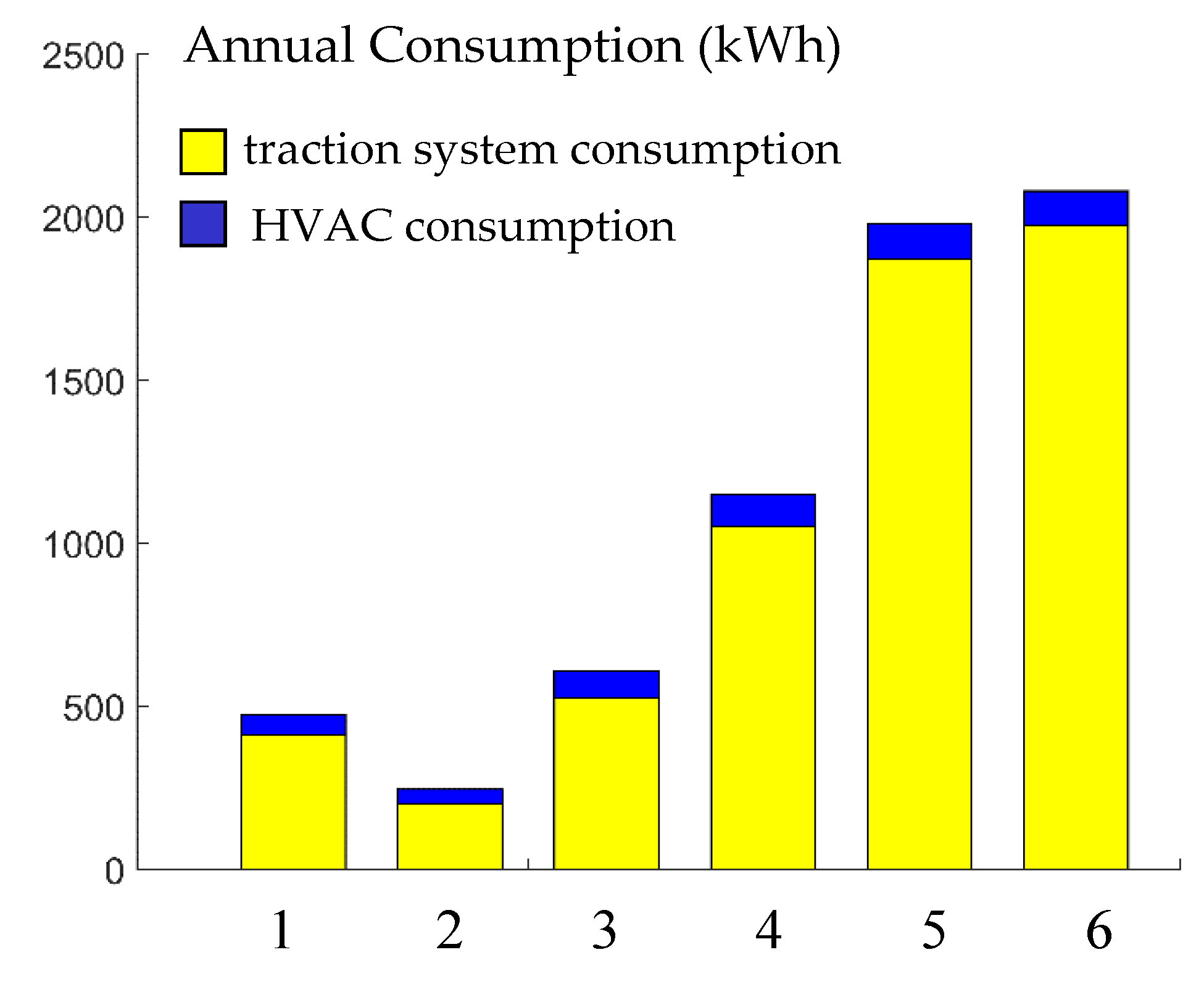
4.2.1. Effect of the HVAC and Traction Subsystems on Consumption

First, the daily energy consumption of the traction subsystem (without HVAC) is calculated for each trip (Figure 12). For a fair comparison of trips with different distances, this consumption is represented in kWh per 100 km. The consumption is impacted by the velocity, which is the most important factor for traction energy consumption, as already demonstrated in [22]. The number of stops also had an impact on the traction consumption of the first trip, leading to a higher consumption than trips 2 and 3.

The energy consumption of the vehicle including both traction and HVAC subsystems each month is given in Figure 13a. for trips 1 and 6. The dashed lines represent the extremum of the energy consumption for the two trips. The energy consumption of trip 1 is globally lower than trip 6. However, the annual variation of trip 1 is larger. For trip 1, in June, the HVAC system is not used at all, leading to the minimal energy consumption of the vehicle. In February, the consumption is highest due to use of the HVAC system. The difference between the consumption of these two months is 21% for trip 1. For trip 6, the variation is only about 8%. The six different trips are compared in Figure 13b. The box represents the extremum of the consumption for each trip. The line inside the box represents the median for the different trips. The variation in energy consumption is largest in the urban trips due to the lower traction consumption and the higher time spent on the road compared to the other trips. This is especially true in trip 1, which has more traffic stops that increase the duration of the trip and represent time when the vehicle is heated but not driven.

4.2.2. Annual Consumption of the Electric Vehicle

Finally, the annual energy consumption is calculated (Figure 14). The yellow parts represent the energy consumption of the traction subsystem while the dark blue bars represent the additional energy used by the HVAC system. The HVAC system adds an average of 12% to the annual energy consumption estimate without the HVAC system. The error varies from 5% for trip 6 to 21% for urban trip 2. These results are for a location with a mild climate that neither requires significant heating nor air conditioning and would be much higher for extreme cases of temperature variation, as in continental climates. This work quantifies the contribution of HVAC energy use to overall consumption and demonstrates that it is not trivial even in a favorable location like Lille, France. Estimates of energy consumption should not neglect HVAC consumption in EVs, especially for urban trips.

5. Conclusions

A simulation tool was developed to study the energy consumption of EVs including energy required for passenger comfort. This model has been validated through a comparison with measured data from a real EV. An analysis of the energy consumption of an electric vehicle that includes the comfort subsystem was performed for an oceanic climate with a temperature variation between −1 °C and 28 °C for different daily trips. The results show the relevance of both driving cycles and climate conditions to energy consumption. Average vehicle velocity has a large effect when the different trips are compared. At the same time, the ambient temperature leads to a higher variation in all types of travel, especially for urban trips, due to the use of the HVAC subsystem. The results for the campus case study here shows an increase in consumption up to 33% in winter due to cabin heating and up to 15% in the summer due to air conditioning. Greater amounts of charging energy should thus be expected in these periods.

Generated driving cycles are used in order to directly and fairly compare between different trips. Consequently, no traffic congestion, no random stops, and no driver effects impacting the driving profile have been considered. These random conditions add even more variation to the energy consumption of the vehicle as they impact both traction and HVAC subsystem consumption. For a daily driving range estimator, the generated driving cycle should be as realistic as possible. This generator can be improved to take into account traffic and driver behavior effects.

In this work, there are several important caveats. First, the analysis focuses on daily commuting trips to the campus of the University of Lille. Reality is more complex as other trips are normally made for different purposes (shopping, collecting children, etc.). Thus, the work can be expanded to other trip types to understand the diversity of trips made by users. The study in this article has addressed a limited temperature range in a moderate climate. The results of this study cannot be directly applied in other climates, particularly for extreme climatic conditions. Moreover, the consumption of the HVAC subsystem increases rapidly when the temperature is below 0 °C and higher than 30 °C [14,15]. Overall, applying these methods outside the mild oceanic climate of Lille should demonstrate stronger effects. In order to extend this to other climates with broader temperature range, two improvements should be pursued. First, a thermal model of the battery should be included as the energy storage and losses are affected at low and high temperature. Second, the control strategies of the HVAC subsystem should be studied in detail because other comfort strategies may be more appropriate for extreme temperature values (such as battery heating).

To conclude, this study quantitatively shows the importance of accounting for the effect of ambient temperature on the energy consumption for daily trips or estimation of the vehicle range. This is relevant for drivers but also for evaluating the design of infrastructure needed to charge a fleet of vehicles. Further works should now be realized to consider the effects of driver behaviors and traffic jams on energy consumption independently of other effects. Then, all effects could be coupled in a comprehensive model.

References

1. Van Mierlo, J.; Messagie, M.; Rangaraju, S. Comparative environmental assessment of alternative fueled vehicles using a life cycle assessment. Transp. Res. Procedia 2017, 25, 3435–3445. [Google Scholar] [CrossRef]
2. Tucki, K.; Orynycz, O.; Świć, A.; Mitoraj-Wojtanek, M. The Development of Electromobility in Poland and EU States as a Tool for Management of CO2 Emissions. Energies 2019, 12, 2942. [Google Scholar] [CrossRef] [Green Version]
3. Global EV Outlook 2020, Entering the Decade of Electric Drive? International Energy Agency Report; International Energy Agency: Paris, France, 2020.
4. C40 Cities Organization. Fossil Fuel Free Streets Declaration. Available online: https://www.c40.org/other/green-and-healthy-streets (accessed on 20 July 2020).
5. Bouscayrol, A.; Castex, E.; Desreveaux, A.; Ferla, O.; Frotey, J.; German, R.; Lhomme, W.; Sergent, J.F. Campus of University with Mobility based on Innovation and carbon Neutral. In Proceedings of the 2017 IEEE Vehicle Power and Propulsion, Belfort, France, 11–14 December 2017. [Google Scholar]
6. Neubauer, J.; Wood, E. The impact of range anxiety and home, workplace, and public charging infrastructure on simulated battery electric vehicle lifetime utility. J. Power Sources 2014, 257, 12–20. [Google Scholar] [CrossRef]
7. Giansoldati, M.; Danielis, R.; Rotaris, L.; Scorrano, M. The role of driving range in consumers’ purchasing decision for electric cars in Italy. Energy 2018, 165, 267–274. [Google Scholar] [CrossRef]
8. Higueras-Castillo, E.; Molinillo, S.; Coca-Stefaniak, J.A.; Liébana-Cabanillas, F. Perceived Value and Customer Adoption of Electric and Hybrid Vehicles. Sustainability 2019, 11, 4956. [Google Scholar] [CrossRef] [Green Version]
9. Kim, S.; Lee, J.; Lee, C. Does Driving Range of Electric Vehicles Influence Electric Vehicle Adoption? Sustainability 2017, 9, 1783. [Google Scholar] [CrossRef] [Green Version]
10. Rauh, N.; Franke, T.; Krems, J.F. User experience with electric vehicles while driving in a critical range situation—a qualitative approach. IET Intell. Transp. Syst. 2015, 9, 734–739. [Google Scholar] [CrossRef] [Green Version]
11. Eisel, M.; Nastjuk, I.; Kolbe, L.M. Understanding the influence of in-vehicle information systems on range stress—Insights from an electric vehicle field experiment. Transp. Res. Part F Traffic Psychol. Behav. 2016, 43, 199–211. [Google Scholar] [CrossRef]
12. Varga, B.O.; Sagoian, A.; Mariasiu, F. Prediction of Electric Vehicle Range: A Comprehensive Review of Current Issues and Challenge. Energies 2019, 12, 946. [Google Scholar] [CrossRef] [Green Version]
13. Yi, Z.; Bauer, P.H. Effects of environmental factors on electric vehicle energy consumption: A sensitivity analysis. IET Electr. Syst. Transp. 2017, 7, 3–13. [Google Scholar] [CrossRef]
14. Kambly, K.; Bradley, T.H. Geographical and temporal differences in electric vehicle range due to cabin conditioning energy consumption. J. Power Sources 2015, 275, 468–475. [Google Scholar] [CrossRef]
15. Yuksel, T.; Michalek, J.J. Effects of regional temperature on electric vehicle efficiency, range, and emissions in the United States. Environ. Sci. Technol. 2015, 49, 3974–3980. [Google Scholar] [CrossRef] [PubMed]
16. Horrein, L.; Bouscayrol, A.; Lhomme, W.; Depature, C. Impact of Heating System on the Range of an Electric Vehicle. IEEE Trans. Veh. Technol. 2017, 66, 4668–4677. [Google Scholar] [CrossRef]
17. Lindgren, J.; Lund, P.D. Effect of extreme temperatures on battery charging and performance of electric vehicles. J. Power Sources 2016, 328, 37–45. [Google Scholar] [CrossRef]
18. German, R.; Shili, S.; Desreveaux, A.; Sari, A.; Venet, P.; Bouscayrol, A. Dynamical Coupling of a Battery Electro-Thermal Model and the Traction Model of an EV for Driving Range Simulation. IEEE Trans. Veh. Technol. 2020, 69, 328–337. [Google Scholar] [CrossRef]
19. Jaguemont, J.; Boulon, L.; Dubé, Y. A comprehensive review of lithium-ion batteries used in hybrid and electric vehicles at cold temperature. Appl. Energy 2016, 164, 99–114. [Google Scholar] [CrossRef]
20. Desreveaux, A.; Bouscayrol, A.; Trigui, R.; Castex, E.; Klein, J. Impact of the Traffic Stops on the Energy Consumption of Electric Vehicles. In Proceedings of the 32nd Electric Vehicle Symposium, Lyon, France, 19–22 May 2019. [Google Scholar]
21. Fernández, R.A.; Caraballo, S.C.; López, F.C. A probabilistic approach for determining the influence of urban traffic management policies on energy consumption and greenhouse gas emissions from a battery electric vehicle. J. Clean. Prod. 2019, 236, 117604. [Google Scholar] [CrossRef]
22. Desreveaux, A.; Bouscayrol, A.; Trigui, R.; Castex, E.; Klein, J. Impact of the Velocity Profile on the Energy Consumption of Electric Vehicle. IEEE Trans. Veh. Technol. 2019, 68, 11420–11426. [Google Scholar] [CrossRef]
23. Fiori, C.; Arcidiacono, V.; Fontaras, G.; Makridis, M.; Mattas, K.; Marzano, V.; Thiel, C.; Ciuffo, B. The effect of electrified mobility on the relationship between traffic conditions and energy consumption. Transp. Res. Part D Transp. Environ. 2019, 67, 275–290. [Google Scholar] [CrossRef]
24. Neubauer, J.; Wood, E. Thru-life impacts of driver aggression, climate, cabin thermal management, and battery thermal management on battery electric vehicle utility. J. Power Sources 2014, 259, 262–275. [Google Scholar] [CrossRef]
25. Liu, K.; Wang, J.; Yamamoto, T.; Morikawa, T. Modeling the multilevel structure and mixed effects of the factors influencing the energy consumption of electric vehicles. Appl. Energy 2016, 183, 1351–1360. [Google Scholar] [CrossRef]
26. De Cauwer, C.; Verbeke, W.; Coosemans, T.; Faid, S.; Van Mierlo, J. A data-driven method for energy consumption prediction and energy-efficient routing of electric vehicles in real-world conditions. Energies 2017, 10, 608. [Google Scholar] [CrossRef] [Green Version]
27. Chan, C.C.; Bouscayrol, A.; Chen, K. Electric, hybrid, and fuel-cell vehicles: Architectures and modeling. IEEE Trans. Veh. Technol. 2010, 59, 589–598. [Google Scholar] [CrossRef]
28. Baouche, F.; Billot, R.; Trigui, R.; El Faouzi, N.E. Efficient Allocation of Electric Vehicles Charging Stations: Optimization Model and Application to a Dense Urban Network. IEEE Intell. Trans. Syst. Mag. 2014, 6, 33–43. [Google Scholar] [CrossRef]
29. Joud, L.; Da Silva, R.; Chrenko, D.; Kéromnès, A.; Le Moyne, L. Smart Energy Management for Series Hybrid Electric Vehicles Based on Driver Habits Recognition and Prediction. Energies 2020, 13, 2954. [Google Scholar] [CrossRef]
30. Chen, Z.; Lu, J.; Liu, B.; Zhou, N.; Li, S. Optimal Energy Management of Plug-In Hybrid Electric Vehicles Concerning the Entire Lifespan of Lithium-Ion Batteries. Energies 2020, 13, 2543. [Google Scholar] [CrossRef]
31. Renault, Z. Available online: http://www.renault.fr/vehicules/vehicules-electriques/zoe (accessed on 20 July 2020).
32. Mayet, C.; Horrein, L.; Bouscayrol, A.; Delarue, P.; Verhille, J.N.; Chattot, E.; Lemaire-Semail, B. Comparison of Different Models and Simulation Approaches for the Energetic Study of a Subway. IEEE Trans. Veh. Technol. 2014, 63, 556–565. [Google Scholar] [CrossRef]
33. Bouscayrol, A.; Hautier, J.P.; Lemaire-Semail, B. Graphic Formalisms for the Control of Multi-Physical Energetic Systems. Systemic Design Methodologies for Electrical Energy, Tome 1, Analysis, Synthesis and Management; Roboam, X., Ed.; ISTE: London, UK; Willey: Hoboken, NJ, USA, 2012; Chapter 3; ISBN 9781848213883. [Google Scholar]
34. EMR Website. Available online: https://www.emrwebsite.org/ (accessed on 20 July 2020).
35. Martínez-García, M.; Zhang, Y.; Gordon, T. Modeling Lane Keeping by a Hybrid Open-Closed-Loop Pulse Control Scheme. IEEE Trans. Ind. Inf. 2016, 12, 2256–2265. [Google Scholar] [CrossRef] [Green Version]
36. Zhang, Q.; Stockar, S.; Canova, M. Energy-Optimal Control of an Automotive Air Conditioning System for Ancillary Load Reduction. IEEE Trans. Control Syst. Technol. 2016, 24, 67–80. [Google Scholar] [CrossRef]
37. Weather Data in Lille in 2018. Available online: https://www.meteofrance.fr (accessed on 20 July 2020).
38. OpenStreetMap API. Available online: https://api.openstreetmap.org (accessed on 20 July 2020).
Figure 1. The studied Renault Zoé before the validation test.
Energies 13 04639 g001
Figure 2. EMR of the traction subsystem.
Energies 13 04639 g002
Figure 3. EMR of the heat pump.
Energies 13 04639 g003
Figure 4. EMR of the comfort subsystem.
Energies 13 04639 g004
Figure 5. Urban driving cycle measured with the vehicle.
Energies 13 04639 g005
Figure 6. Vehicle cabin temperature.
Energies 13 04639 g006
Figure 7. Measured and simulated energy consumption for the urban driving cycle.
Energies 13 04639 g007
Figure 8. Average minimal and maximal temperature per month in Lille in 2018 [37].
Energies 13 04639 g008
Figure 9. Simulation process: (a) map-based trip selection, (b) deduced velocity profile, (c) vehicle simulation.
Energies 13 04639 g009
Figure 10. Monthly variation in the EV energy consumption for the urban trip.
Energies 13 04639 g010
Figure 11. Different outgoing trips considered in this study.
Energies 13 04639 g011
Figure 12. Energy consumption of the traction subsystem in the six sample trips.
Energies 13 04639 g012
Figure 13. (a) Energy consumption of the Electric Vehicle over 12 months of the year for trips 1 and 6. The dashed lines represent the extremum of the energy consumption for each trip. (b) Energy consumption of the Electric Vehicle for 6 different trips. The boxplot represents the extremum of the energy consumption for the different trips. The lines inside the boxes represent the median.
Energies 13 04639 g013
Figure 14. Annual energy consumption of the Electric Vehicle in the 6 commuting trips.
Energies 13 04639 g014