A Model of a Diaphragm Wall Ground Heat Exchanger ^†

Abstract

Ground thermal energy is a sustainable source that can substantially reduce our dependency on conventional fuels for heating and cooling of buildings. To exploit this source, foundation sub-structures with embedded heat exchanger pipes are employed. Diaphragm wall heat exchangers are one such form of ground heat exchangers, where part of the wall is exposed to the basement area of the building on one side, while the other side and the further depth of the wall face the surrounding ground. To assess the thermal performance of diaphragm wall heat exchangers, a model that takes the wall geometry and boundary conditions at the pipe, basement, and ground surfaces into account is required. This paper describes the development of such a model using a weighting factor approach, known as Dynamic Thermal Networks (DTN), that allows representation of the three-dimensional geometry, required boundary conditions, and heterogeneous material properties. The model is validated using data from an extended series of thermal response test measurements at two full-scale diaphragm wall heat exchanger installations in Barcelona, Spain. Validation studies are presented in terms of comparisons between the predicted and measured fluid temperatures and heat transfer rates. The model was found to predict the dynamics of thermal response over a range of operating conditions with good accuracy and using very modest computational resources.

1. Introduction

Exploiting sustainable sources of energy with the potential to contribute to the heating and cooling of buildings—the major contributing factor to energy consumption in developed countries [1]—is one of the major challenges of the world today, so reduction in such demands is a key element of most national emission reduction strategies. Building thermal energy systems that rely on heat pumps and some form of ground heat exchanger is one of the most effective means of implementing energy-efficient building thermal systems [1,2,3]. Of the various types of ground heat exchangers that are in use, making use of building sub-structure (foundation) elements is one of the most attractive options for larger buildings [4,5]. A number of types of sub-structural building elements have been used as the bases of ground heat exchangers, including piles, diaphragm walls, and ground-coupled slabs [6]. Using substructures as heat exchangers dates back to the 1980s, when ground-bearing slabs were employed to exchange heat with the ground, followed by further advancements until 1996, when the first diaphragm walls equipped with heat exchanger pipes were examined in Austria and Switzerland [7].

Although various studies have been conducted to investigate the performance of thermally activated piles [8,9,10,11], diaphragm wall heat exchangers (DWHE) have received less interest [5]. One of the first studies that focused on heat transfer in diaphragm walls corresponds to the work of Brandl [7]. In this work, diaphragm walls were applied in three main pilot projects, including a rehabilitation centre, a railway tunnel, and metro stations. Brandl [7] also reported further smaller projects. Later in 2009, Adam and Markiewicz [4] carried out finite element analysis to investigate the heating and cooling performance of diaphragm walls with differing heat exchanger pipe spacings. They summarised that the thermal power tends to decrease with larger distances, with the installation cost tending to an optimum. Nevertheless, they pointed out that although the method is applicable to any geothermal system installed in foundation elements, these findings are only rational for the studied case and may vary remarkably for others. The first experimental explorations of heat transfer characteristics of DWHEs were carried out by Xia et al. [12] using borehole heat exchangers (BHE) as benchmarks. Xia et al. [12] highlighted the factors influencing heat exchange rate in such geostructures. A model for two-dimensional heat transfer in DWHEs validated against numerical solutions and measured data was proposed by Sun et al. [13] based on the structural features of the wall, i.e., over and under the excavation line. Although the temperature profiles predicated by their model show limited consistency with the experimental data, it was considered as adequate by the authors.

A numerical method to investigate thermal performance of DWHEs was presented by Kürten et al. [14], and was validated against laboratory results. The authors of Bourne-Webb et al. [15] compared the methods used for evaluating BHEs and energy geostructures, and outlined their commonalities and differences. In a different research, Bourne-Webb et al. [16] carried out numerical studies to demonstrate the heat transfer procedure in DWHEs, and reported that the key process is the one between the the air-void and the wall rather than the ground. A coupled thermo-mechanical analysis was employed by Coletto and Sterpi [17] to investigate how the heat transfer affects the soil temperatures, the wall internal actions, and the soil–structure interaction. Di Donna et al. [18] detailed the key parameters controlling the energy efficiency in DWHEs through numerical investigations and statistical analysis.

Soga and Rui [5] summarised the status of the understanding of the thermal conduct of energy geostructures and discussed some design considerations. It was recommended that further investigations need to be carried out to increase the reliance on using such substructure heat exchangers. Sterpi et al. [19] investigated the energy performance as well as short and long term influence on the soil temperatures using finite element thermal analysis. Furthermore, they carried out finite element thermo-mechanical analysis to highlight the wall’s geotechnical and structural response. In a more recent research, Sterpi et al. [20] explored different factors influencing the performances of DWHEs, which include the pipe arrangements in the wall, the ratio between exposed and fully immersed parts of the wall, and the variable thermal condition on the excavation side. To that end, they employed finite volume analysis using a full-scale monitored diaphragm wall as a reference. Their findings detailed an improved layout for the pipe so that the heat exchange rate could be enhanced by 15.8% for their studied case. Moreover, they showed that other factors which contribute to improving heat transfer characteristics of the wall include limiting the thermal interference between pipe branches that carry fluid at different temperatures and using both faces in the fully immersed part of the wall that are in direct contact with the soil.

Rammal et al. [21] reported that presence of major groundwater flow and having the whole length of diaphragm wall activated have a positive impact on the heat exchange rate, while the thermal performances of the walls are directly affected by the amount of thermal load. Barla et al. [22] investigated the energy efficiency of DWHEs using finite element thermo–hydro coupled analyses in addition to the effects of the thermal activation on the surrounding soil. Furthermore, they employed finite difference thermo-mechanical analyses to study the mechanical effects induced by the thermal activation. They reported that horizontal pipe layout will maximise the heat exchange rates. Kürten et al. [23] presented a thermal resistance model based on rotational symmetry, number of pipes, and the spatial separation, and implemented it into a finite difference code; however, their model does not take seasonal fluctuation of the near-surface temperature and the groundwater into account.

In modelling the thermal conditions of DWHE, review of the literature highlights that a number of different assumptions can be made about the boundary conditions, geometric complexity, fluid flow, and heterogeneity of properties. In developing a new model, the objectives were to: (i) Facilitate adequate boundary conditions, (ii) represent geometric complexity, and (iii) achieve computational efficiency. The advantages of ground heat exchange are often stated in terms of the stability of the ground temperatures and decoupling from varying atmospheric conditions. This is arguably true of deeper ground heat exchangers such as borehole heat exchangers, but is questionable in the case of diaphragm walls. Kasuda and Archenbach [24] demonstrated that ground temperature variations driven by seasonal variation in environmental conditions at the ground surface penetrate in an observable way as much as 10 m below the surface. In view of this, we sought to incorporate time-varying boundary conditions at the upper ground surface. A further consideration included thermal conditions related to the building basement surfaces. As these are sheltered from environmental conditions (e.g., solar irradiation) and air temperatures are moderated, conditions are likely to be different from those at the ground surface. Furthermore, the basement conditions are rather different from ground conditions, so significant temperature differences can exist where the DWHE is exposed to the basement on one side and coupled to the ground on the other. Consequently, three different surface conditions are considered: Outside the building where the ground is exposed to solar irradiation and precipitation, adjacent basement spaces where there is isolation from such effects but exposure to the internal air temperatures, and finally, the pipe/fluid interface surfaces where heat is exchanged with the heating and cooling system.

In developing an energy-pile-based heating and cooling system with respect to thermal performance, response to the time-varying heat transfer rates imposed by the building system is the chief concern. To understand minimum and maximum fluid temperatures requires calculation of short timescale effects (hourly or sub-hourly variations); understanding long-term sustainability requires calculation over very long timescales. Calculation methods that can deal with this difference in timescales with sufficient computational efficiency to allow design calculations and optimisation are needed. This tends to preclude direct application of three-dimensional numerical models.

Widely adopted approaches to the thermal design and simulation of ground heat exchange systems of the borehole type include applying reduced-order or response-factor methods. Reduced-order approaches include one- or two-dimensional numerical models and lumped capacitance–resistance networks [25] or hybrid approaches that also use response-factor methods [26]. The approaches that can be classified as response-factor methods all rely on spatial and temporal superposition of responses to some form of heat flux or temperature pulse. The definition of unit heat flux step pulse responses in so-called ’g-functions’ [27] has been applied to energy-pile design calculations [28,29]. However, this form of response factor is less appealing in the case of DWHE, as it only allows consideration of one time-varying boundary condition (at the borehole wall or pipes) and assumes that the upper ground surface has a constant temperature.

In order to meet the modelling objectives identified above, the proposed DWHE model is based on a response-factor approach known as a Dynamic Thermal Network (DTN). This allows for multiple boundary condition surfaces, arbitrary geometries, and heterogeneous thermal properties. The basis of the method is summarised in the following section of the paper; further details are available in reports of earlier work [30,31]. In order to validate the model, experimental heat transfer data was collected from two full-scale DWHE installations in a range of conditions representative of realistic operation. This validation study is presented later in this paper.

2. Model Development and Dynamic Thermal Network Representation

The concept of representing heat transfer as a network of nodal temperatures and resistances is extended in the Dynamic Thermal Network (DTN) approach to deal with transient conduction in heterogenous solid bodies where the heat fluxes are driven by time-varying boundary temperatures. The concept and the underlying mathematical principles were developed by Claesson [32,33,34] and Wentzel [35], and were demonstrated through application to building and ground heat transfer modelling applications. The heat conduction problem for this class of problems can be formulated according to Fourier’s Law with constant properties and a set of N mixed boundary conditions with constant surface heat transfer coefficients, h, as follows:

$$\begin{array}{cc}\hfill \mathsf{\nabla }\left(\lambda \mathsf{\nabla }T\right)& =\rho C\frac{\partial T}{\partial t}\hfill \end{array}$$

(1a)

$$\begin{array}{cc}\hfill h_i\left[T_i{\left(t\right)-T|}_{S_i}\right]& =\lambda \frac{\partial T}{\partial n},[i=1\dots N].\hfill \end{array}$$

(1b)

In this form of conduction problem, the primary interest is in the relationship between boundary fluxes and temperatures rather than internal body temperatures. Once the differential equation has been solved to find the temperatures, the boundary heat fluxes of interest can be calculated, simply using

$$\begin{array}{cc}\hfill Q_i\left(t\right)& =S_i{h}_i\left[T_i{\left(t\right)-T|}_{S_i}\right]\hfill \end{array}$$

(2)

2.1. Model Description

The network representation of a body with three boundary surfaces is illustrated in Figure 1. One of the essential features of the DTN method is that heat fluxes at each surface are separated into admittive (or absorptive) and transmittive components. Admittive fluxes are associated with variations in temperature at that boundary. In the case of an adiabatic surface, the only fluxes are the variations brought about by variations in boundary temperature at that surface. In this case, the fluxes are entirely admittive in nature, and the transmittive component is zero. Where there is heat transfer with another surface, an additional component is superimposed depending on the difference between the boundary temperatures. This is the transmittive component and is the flux observed at the opposing surface. In general, both components of the heat flux are present. In steady-state conditions, the admittive component is zero and the fluxes at all of the surfaces are transmittive in nature.

The conductances in the admittive path of the network are denoted with a single subscript $K_i$ and are equal to the surface area multiplied by a constant heat transfer coefficient, e.g., $K_1=S_1{h}_1$. There are constant conductances between each pair of surfaces, denoted with double subscripts $K_{ij}$, along the transmittive path. These conductances are the overall steady-state conductances between the boundaries, and include the surface conductances $K_i$ and $K_j$. The reversed summation symbols ($\mathsf{\Sigma }$) adjacent to the conductances in Figure 1 indicate that the driving temperatures are averages of the current and previous temperatures. In the single-ended admittive path, the single summation sign indicates that the driving temperature is a function of the average temperature at that boundary alone.

Another feature of the DTN approach is that the temperatures ($T_i\left(t\right)$) and fluxes ($Q_i\left(t\right)$) of the dynamic network are defined at boundary (or environmental) temperature nodes rather than at the surfaces themselves. We accordingly make a distinction between the terms ’boundary’ and ’surface’ in the following discussion. For a model of a diaphragm wall heat exchanger, we define three surfaces at which different time-varying boundary conditions are applied. It is sufficient to represent the pipe system as a single boundary surface. For this application, the ground is thought to have a more significant influence on thermal conditions—at least at longer time scales—and so we define this as one boundary. The other boundary of interest is that at which the wall is exposed to conditions in the associated building basement. This concept is illustrated in Figure 2.

The nodal heat balance equations set out the relationship between the total flux at each boundary and the admittive and transmittive components. For a three-surface problem, the heat balance equations are:

$$\begin{array}{cc}\hfill Q_1\left(t\right)& =Q_{1a}\left(t\right)+Q_{12}\left(t\right)+Q_{13}\left(t\right)\hfill \\ \hfill Q_2\left(t\right)& =Q_{2a}\left(t\right)+Q_{21}\left(t\right)+Q_{23}\left(t\right)\hfill \\ \hfill Q_3\left(t\right)& =Q_{3a}\left(t\right)+Q_{31}\left(t\right)+Q_{32}\left(t\right).\hfill \end{array}$$

(3)

It is helpful to understand the relationship between the admittive and transmittive fluxes by considering the responses to a step change in boundary temperature at one of the surfaces. The response for a three-surface body excited in this way is illustrated in Figure 3. At the beginning of the step change, the flux at the surface being excited is entirely admittive in nature and is limited by the surface conductance ($h_i{S}_i$). At any time, the admittive component is given by the difference between the total surface flux and the sum of the transmittive fluxes at the other surfaces. As steady-state is approached, the admittive flux approaches zero and the transmittive flux to the other two surfaces approaches the steady-state value. The specific case of fluxes in a diaphragm wall with the step change applied at the pipe surface is shown in Figure 4. The steady-state pipe flux can be seen to be balanced by the combination of basement and ground fluxes.

Claesson [33] showed that the temperature differences driving the absorptive and transmittive fluxes can be defined in an exact manner by the current and weighted averages of the boundary temperatures. The absorptive and transmittive fluxes at a given boundary can be written in terms of the conductances and these temperatures, as follows:

$$\begin{array}{cc}\hfill Q_{ia}\left(t\right)& =K_i\left(T_i\left(t\right)-\underset{0}{\overset{\infty }{\int }}{\kappa }_{ia}\left(\tau \right)T_i(t-\tau )d\tau \right)\hfill \end{array}$$

(4)

$$\begin{array}{cc}\hfill Q_{ij}\left(t\right)& =K_{ij}\underset{0}{\overset{\infty }{\int }}{\kappa }_{ij}\left(\tau \right)\left[T_i(t-\tau )-T_j(t-\tau )\right]d\tau .\hfill \end{array}$$

(5)

These weighted average temperatures are those associated with the points in the network indicated by a reversed summation symbol (Figure 1). The temperatures are averaged according to weighting functions, ${\kappa }_{ia}$ and ${\kappa }_{ij}$ for the admittive flux at the surface and the transmittive flux between surfaces, respectively. A shorthand notation is used to denote these weighted average temperaturesS as follows:

$$\begin{array}{cc}\hfill {\overline{T}}_{ia}\left(t\right)& =\underset{0}{\overset{\infty }{\int }}{\kappa }_{ia}\left(\tau \right)T_i(t-\tau )d\tau \hfill \end{array}$$

(6)

$$\begin{array}{cc}\hfill {\overline{T}}_{ij}\left(t\right)& =\underset{0}{\overset{\infty }{\int }}{\kappa }_{ij}\left(\tau \right)T_i(t-\tau )d\tau .\hfill \end{array}$$

(7)

Using this notation and substituting Equations (4) and (5) into Equation (3) allows the heat balance equations for each surface to be expressed as:

$$\begin{array}{cc}\hfill Q_1\left(t\right)& =K_1\left[T_1\left(t\right)-{\overline{T}}_{1a}\left(t\right)\right]+K_{12}\left[{\overline{T}}_{12}\left(t\right)-{\overline{T}}_{21}\left(t\right)\right]\hfill \\ \hfill & +K_{13}\left[{\overline{T}}_{13}\left(t\right)-{\overline{T}}_{31}\left(t\right)\right]\hfill \\ \hfill Q_2\left(t\right)& =K_2\left[T_2\left(t\right)-{\overline{T}}_{2a}\left(t\right)\right]+K_{12}\left[{\overline{T}}_{21}\left(t\right)-{\overline{T}}_{12}\left(t\right)\right]\hfill \\ \hfill & +K_{23}\left[{\overline{T}}_{23}\left(t\right)-{\overline{T}}_{32}\left(t\right)\right]\hfill \\ \hfill Q_3\left(t\right)& =K_3\left[T_3\left(t\right)-{\overline{T}}_{3a}\left(t\right)\right]+K_{13}\left[{\overline{T}}_{31}\left(t\right)-{\overline{T}}_{13}\left(t\right)\right]\hfill \\ \hfill & +K_{23}\left[{\overline{T}}_{32}\left(t\right)-{\overline{T}}_{31}\left(t\right)\right].\hfill \end{array}$$

(8)

It can be seen that in the steady-state, Equation (8) reduces to the usual expression for flux in terms of overall conductance and boundary temperatures ($Q_1=K_{12}(T_1-T_2)+K_{13}(T_1-T_3)$, etc.).

2.2. Discretisation

A convenient way to derive suitable weighting functions is to consider the fluxes resulting from step changes in boundary temperatures. All of the required weighting functions can be found by applying the step boundary condition at one of the surfaces and holding the other boundary temperatures at zero, and repeating this for each surface (as in Figure 3). Claesson [33,34] showed that the calculation method could be expressed in discrete form, in an exact way, for piecewise linear variations in boundary conditions. The weighting factors can be obtained using the admittive and transmittive fluxes calculated from the step responses averaged over each step (size $\mathsf{\Delta }t$). The discrete weighting factors are then obtained from the differences in these average time step fluxes as follows:

$$\begin{array}{cc}\hfill {\kappa }_{ia,\rho }& =\frac{{\overline{Q}}_{ia}\left(\phi \right)-{\overline{Q}}_{ia}\left(\omega \right)}{{\overline{K}}_i}\hfill \\ \hfill {\kappa }_{ij,\rho }& =\frac{{\overline{Q}}_{ij}\left(\omega \right)-{\overline{Q}}_{ij}\left(\phi \right)}{K_{ij}},\hfill \end{array}$$

(9)

where the time differences are between $\phi =(\rho \mathsf{\Delta }t-\mathsf{\Delta }t)$ and $\omega =\rho \mathsf{\Delta }t$. In the case of the admittive weighting factors, a modified surface conductance (${\overline{K}}_i$) is defined which is equal to the initial admittive flux, ${\overline{K}}_i={\overline{Q}}_{ia}\left(0\right)$.

When the boundary temperatures are defined by a discrete time series, the average temperatures are calculated by the summation of weighting factor sequences multiplied by boundary temperature sequences that represent the state at previous time steps. The discrete form of Equations (6) and (7) is, for current time step n,

$$\begin{array}{cc}\hfill {\overline{T}}_{ia,n}& =\sum _{\rho =1}^{\infty }{\kappa }_{ia,\rho }{T}_{i,n-\rho }\hfill \end{array}$$

(10)

$$\begin{array}{cc}\hfill {\overline{T}}_{ij,n}& =\sum _{\rho =0}^{\infty }{\kappa }_{ij,\rho }{T}_{i,n-\rho }\hfill \end{array}$$

(11)

This process of updating the temperature history can be implemented in a very computationally efficient manner. For a given set of boundary temperatures, the fluxes can then be calculated using Equation (8). Again, these are very simple algebraic equations that are efficiently calculated.

2.3. Boundary Conditions

The DTN is formulated and the step response data are calculated assuming that surface heat transfer coefficients ($h_i$) are constant. The general approach we took to work around this assumption was to define a boundary temperature that is an ‘effective temperature’ ($T_e$) that, when applied using the predefined constant heat transfer coefficient, gives the same expected surface heat flux as that of applying a more complex boundary condition model. This effective temperature (or environmental temperature) does not correspond directly to a physical boundary temperature, but is applied in the DTN heat balance equations and when the weighted average temperature is updated. In this application, we do this using slightly different formulations for the pipe, ground, and basement boundaries. The initial values of $h_i$ used for calculating the weighting factors were chosen as mid-range values in comparison with those expected in the simulations: 1000 W m${}^{-2}$ K${}^{-1}$ for the pipe surface and 10.0 W m${}^{-2}$ K${}^{-1}$ for the other surfaces exposed to the external environment. These values are somewhat arbitrary, as we modify the simulation values as described below.

At surfaces exposed to the external environment, convection processes act in combination with short-wave and long-wave radiant fluxes. A surface heat balance defining such a boundary condition is

$$\begin{array}{cc}\hfill \frac{Q_i}{S_i}& =R_{sw}+R_{lw}+h_{ca}\left(T_a-T_{Si}\right).\hfill \end{array}$$

(12)

The effective boundary temperature is intended to give the equivalent heat flux and is hence defined by,

$$\begin{array}{cc}\hfill \frac{Q_i}{S_i}& =h_i\left(T_e-T_{Si}\right).\hfill \end{array}$$

(13)

Hence, the equivalent or environmental temperature must be

$$\begin{array}{cc}\hfill T_e& =[R_{sw}+R_{lw}+h_{ca}{T}_a+\left(h_{ca}-h_i\right)T_{Si}]/h_i.\hfill \end{array}$$

(14)

A correlation for convection over a flat surface has been used to find the value for the ground surface in this case: $h_{ca}=11.58+5.89U_w$, where $U_w$ is the wind speed [36].

This external surface boundary condition formulation can be expanded to deal with evapotransporation [31]. At the basement surface, we apply a reduced form of this expression, which ignores solar and long-wave radiation. This simplification was made to deal with the limitations of the validation tests—described later—that were carried out during the construction process, i.e., before a building over the foundations was finished.

In geometries with embedded pipes like a diaphragm wall, it is necessary to define the relationship between the boundary temperature and both the pipe fluid inlet and outlet temperatures. Our approach is—similarly to that of Strand [37]—to assume that the pipe surface temperature does not vary along its length and make an analogy with an evaporating–condensing heat exchanger, and so to define a characteristic effectiveness parameter. The pipe fluid heat balance is then defined by the maximum possible temperature difference and the effectiveness, as follows:

$$\begin{array}{c}\hfill Q_p\left(t\right)=\epsilon \dot{m}C\left(T_{in}\left(t\right)-T_p\left(t\right)\right),\end{array}$$

(15)

where the subscript p refers to the pipe. For such a heat exchanger, $\epsilon =1-e^{-NTU}$; this is related to the total pipe area and fluid heat transfer coefficient by the Number of Transfer Units ($NTU=\left(2\pi rH{h}_p\right)/\left(\dot{m}C\right)$), where H is the length of the pipe. The pipe convection coefficient, $h_p$, is modelled using the well-known Dittus–Boelter equation such that

$$\begin{array}{c}\hfill h_p=\frac{0.023R{e}^{4/5}P{r}^n{k}_f}{2\pi r_p},\end{array}$$

(16)

where the exponent, n, is $0.4$ or $0.3$, according to the heat transfer being by heating or cooling.

In the implementation of the diaphragm wall model, we use the outside of the pipe (i.e., the concrete cylindrical surface) as the boundary and calculate an equivalent heat transfer coefficient to take account of the thermal resistances of the fluid and pipe materials. This is possible by rearranging the heat balance equations to calculate the effective pipe boundary temperature in a way that avoids iteration using only the inlet temperature as the time-varying input data. The outlet temperature can then be found from the fluid heat balance: $T_{out}\left(t\right)=T_{in}\left(t\right)-Q_P\left(t\right)/\left(\dot{m}C\right)$. This approach to the treatment of pipe boundary conditions was tested and validated in a different form of ground heat exchanger application reported in [31].

2.4. Derivation of Discrete Weighting Factors

Derivation of the weighting factors for the DTN method can be done by analysis of step responses at each boundary in turn. The method used to calculate the step response can vary: Both analytical and numerical methods were used. In this case, we used a numerical model for this task. To make this efficient, we implemented a parametric method of mesh generation for simple diaphragm wall geometries and used the OpenFOAM library [38] to calculate conduction heat transfer over long timescales. The solver was adapted to use increasing time steps to make the process efficient.

The parametric mesh generation tool generates the required geometry and mesh definition given basic heat exchanger design parameters (pipe diameter and depth, wall depth and thickness, pipe spacing, and basement depth). The mesh is generated assuming that the wall has symmetry planes between the vertical pipes. An example of the mesh showing the definitions of the three surfaces used to apply the boundary conditions is shown in Figure 5. The number of cells in the meshes is of the order of one million. The overall domain size is three times the depth of the wall to ensure that sufficient ground material is considered.

It is assumed that some symmetry to the geometry is representative of most wall sections, except those at the corner of the plot, where three-dimensional effects can be expected and may become more important at long time scales. In the validation studies, wall sections were tested that were not thought to be influenced by conditions near the corners of the plot. This is not a limitation of the modelling approach per se; corner effects could be dealt with by using a more complex mesh generation method.

Having generated three sets of response data in the form of heat flux time series (as in the example shown in Figure 4), discrete weighting factors were calculated for the chosen time step size using Equation (9). The details of this process and how the weighting factors were reduced to a compact data set are described by Wentzel [35] and Rees and Fan [30]. An illustration of the weighting factor series for the admittive flux of a diaphragm wall is shown in Figure 6.

2.5. Model Implementation

Generation of the discrete weighting factor series values is a preliminary step in the modelling process that only has to be executed once. A library of such data can be developed for particular geometry and thermal property variations for repeated application in modelling exercises. Conducting a modelling exercise (i.e., making long-term predictions of fluid temperatures and heat transfer rates for given inlet temperatures and flow rates) is carried out in relatively simple coding that reads the weighting factors and implements the heat balance Equations (4) and (5), along with the boundary conditions Equations (14) and (15). This was implemented as a stand-alone application and also in the form of a component model in the TRNSYS simulation environment [39]. A flow chart describing the DTN modelling process is shown in Figure 7.

3. In-Situ Thermal Response Measurements

In order to both test the capabilities of a prototypical diaphragm wall heat exchanger design and generate validation data for the model, a series of thermal response measurements were made on a total of four wall sections at two sites in Barcelona, Spain. The objective was to activate the heat exchanger using a series of heat pulses and to measure flow rates and fluid temperature responses. The apparatus used to apply the heat pulses and record the data was similar to that used for in-situ estimation of ground thermal properties. However, the objective was to simulate operating conditions rather than to indirectly measure ground thermal properties. Ground thermal properties were measured independently, as described below.

3.1. Test Site Installations

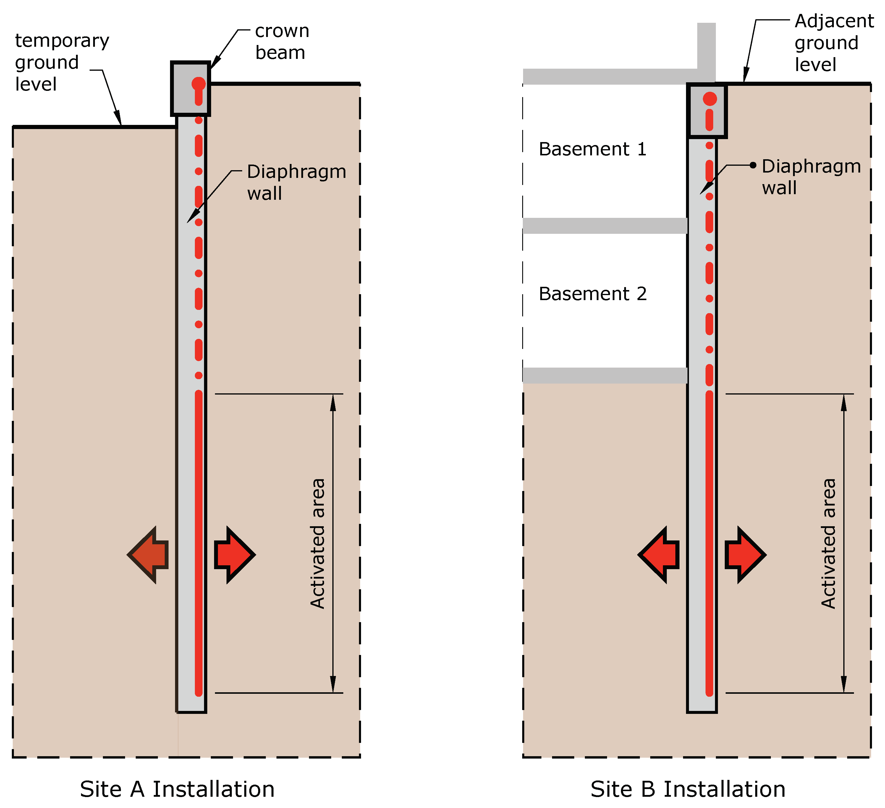
The first series of response tests were carried out at a full-scale prototype installation at a road construction project (Gran Via de les Corts Catalanes) in the Glorias (Glòries) district; we denote this ‘Site A’ hereafter. At this site, two screen walls of 40 m depth were activated. The tests were performed from September 2016 to November 2016. In this case, as the diaphragm wall did not form part of a building system, tests were carried out during the road construction project with ground material on both sides of the wall, i.e., before final excavation.

The second and larger test site was at a complex of four office buildings of 12,700 m${}^2$ floor area located in the 22@ district of Barcelona; we denote this ‘Site B’ hereafter. A total of 37 diaphragm walls (around 770 m${}^2$ active area) were installed in this building project—19 of which are conventional diaphragm walls around the perimeter, and 18 of which are below the lowest basement floor, supporting a central section of the building. The perimeter wall sections are exposed to two levels of basement parking space in their upper section, whereas the basement sections are (like piles) surrounded by ground material on all sides and covered by the lower basement slab. The depths of the wall sections vary between 15 and 17.5 m for those under the basement and 14.5–18 m for those at the perimeter of the basement. Testing of individual wall sections began in July 2017 and lasted until April 2018. The monitoring of whole system’s performance has continued into 2019.

Two different arrangements of heat exchanger piping were used at the test sites. At Site A, the pipe was attached to the outside of the reinforcement in a parallel vertical pattern. At Site B, a different arrangement was tested, which used a horizontal parallel arrangement. In all cases, the pipe was a nominal 25 mm diameter cross-linked polyethylene (PEX) material. The general arrangement of the walls and heat exchange elements at both sites are shown in Figure 8. The geometric parameters for each installation are given in Tables 2 and 3. At Site A, there are accordingly six vertical pipes in the lower half of the wall, giving a total pipe circuit length of 82 m. This is a practical length that can be achieved without pipe joints in the wall.

The wall sections are assembled from two sections of reinforcement cage with the pipe fixed in a serpentine arrangement in the lower half only, as indicated by the active area in Figure 8. At Site B, this means that the activated area is below the bottom of the basement. Pairs of flow and return connecting pipes pass vertically through the upper section and are terminated in a crown beam structure. At Site A, the wall section was one section in a row of similar wall sections. At Site B, the wall sections activated for thermal testing were mid-way along the perimeter, so that the complications of 3D heat transfer that can occur at the corners of the plot at longer time scales could be avoided.

3.2. Thermal Response Test Equipment

A new thermal response test system was developed for this project. The design of the equipment consists of a water tank with electric heaters and a circulation pump, along with instrumentation and data logging equipment. During the tests, inlet temperature was measured, as well as the flow rate and the return temperature, so thermal power exchanged with the ground and the evolution of the inlet and outlet temperatures as the heat flow modifies thermal conditions could be measured. The system is shown schematically in Figure 9.

The test equipment was designed to be as robust and reliable as possible due to the weather conditions faced during long periods at the construction sites and is shown in Figure 10. The system was designed to operate with site power or generator electrical supplies and a heater capacity of 0.5, 2.0, 2.5, or 4.0 kW. After initial tests, it was decided to conduct tests on individual heat exchanger sections (a single circuit of up to 100 m pipe length) with a constant heat input of 2.0 or 2.5 kW and with the pump set for a constant flow. This ensured that the maximum temperatures were in the range 30–40 °C and the flow was in the turbulent regime ($Re$ > 2000), with a fluid temperature difference of 4–5 °C in order to minimise uncertainties. Tests in Barcelona were conducted with plain water as the heat transfer fluid. Heat input was arranged to automatically cycle between on and off conditions over periods varying from 2 h to 1 wk in order to simulate a range of realistic operating conditions, as elaborated below.

3.3. Material Characterisation

We sought to independently measure the relevant thermal properties of both the wall concrete and ground materials. This was done through a series of laboratory tests using samples from Site A and Site B. The primary properties of interest are the thermal conductivity and specific heat of the materials. Both the Transient Plane Source Method (TPSM) [40] and Transient Line Source Method (TLSM) [41] were used to measure thermal conductivity. It was found that the TPSM method was best suited to testing the concrete sample (600 × 600 × 40 mm) and that the TLSM was best suited to testing the porous ground material. In order to measure specific heats, the Differential Scanning Calorimetry (DSC) method was applied [42]. Results from these tests are shown in

Table 1. Ground material and concrete thermal property measurement results, Site A.

Material	Method	Property	Value	Units
Concrete	TPSM	thermal conductivity ($\lambda$)	1.90	W m${}^{-1}$ K${}^{-1}$
Concrete	TLSM	thermal conductivity ($\lambda$)	2.48	W m${}^{-1}$ K${}^{-1}$
Ground	TPSM	thermal conductivity ($\lambda$)	0.86–0.91	W m${}^{-1}$ K${}^{-1}$
Ground	TLSM	thermal conductivity ($\lambda$)	1.46	W m${}^{-1}$ K${}^{-1}$
Concrete	DSC	specific heat (C)	0.85	kJ kg${}^{-1}$ K${}^{-1}$
Ground	DSC	specific heat (C)	0.81	kJ kg${}^{-1}$ K${}^{-1}$
Concrete	literature	density ($\rho$)	19.5–24.0	kN m${}^{-3}$
Ground	measured	density ($\rho$)	19.5	kN m${}^{-3}$
Concrete	calculated	heat capacity ($\rho C$)	1.69–2.08	MJ m${}^{-3}$ K${}^{-1}$
Ground	calculated	heat capacity ($\rho C$)	1.61	MJ m${}^{-3}$ K${}^{-1}$

.

At Site B, it was not possible to retrieve a suitable sample of ground material due to the complexities of the ongoing construction process. Considering the closeness of Sites A and B (900 m) and the reported similarity of the ground materials, the ground thermal properties for Site B were taken to be the same as Site A. This assumption and the possibility of higher groundwater levels at Site B introduce additional uncertainty in the effective property values, however.

The concrete samples tested did not include any reinforcement steel, so studies were performed to obtain values of conductivity and heat capacity for the composite wall (treated as one homogeneous material in the model) using rules of mixtures [43] and knowledge of the reinforcement design. The density of the composite wall was given exactly by an arithmetic mean weighted by the volume fraction of the wall material. A similar approach was used to obtain the value for heat capacity. An exact value for thermal conductivity of a composite material can not be achieved, and such values lie between those of its constituents. Therefore, for a diaphragm wall, the thermal conductivity value is in the range between those of concrete and steel. To achieve an appropriate value of thermal conductivity for the diaphragm wall in the model, various values between the upper and lower bounds were tested, which also provided knowledge on the sensitivity of the DTN model to such values.

4. Validation Study Results

The validation of the model presented is firstly based on the study of Site A. This site has well-defined independently measured thermal property values available. At Site B, we took a slightly different approach, and parametrically investigate sensitivity to the more uncertain thermal property values to show that the model is able to reproduce the experimental results given justifiable assumptions about these values.

Validation calculations were performed for Site A using thermal conductivity values ranging from 1.9–2.48 Wm${}^{-1}$ K${}^{-1}$ for concrete and 0.86–1.46 Wm${}^{-1}$ K${}^{-1}$ for ground. These values represent the range measured in the lab tests of the site samples using the TLSM and TPSM approaches (Table 1). As laboratory measurements of the concrete density were not available, density values of 19.50, 22.00, and 24.00 kNm${}^{-3}$ were applied, while one single density value of 19.50 kNm${}^{-3}$ was used for the ground.

The initial results indicated that there is sensitivity to both the concrete and the ground thermal conductivities, and the closest agreement was found with a higher value of ground thermal conductivity and lower value of concrete thermal conductivity. These are the values that correspond to those obtained by the TPSM for concrete and TLSM for the ground. These are the test methods expected to be the most appropriate for solid and porous materials, respectively, as noted earlier. In addition, the best agreement was found at higher values of concrete density. Accordingly, a ground conductivity of 1.46 Wm${}^{-1}$K${}^{-1}$, a reinforced concrete conductivity and volumetric heat capacity of 2.0 Wm${}^{-1}$K${}^{-1}$ and 2.1 MJm${}^{-3}$K${}^{-1}$, respectively, and a concrete density of 24.00 kNm${}^{-3}$ were applied in the final validation study. The use of the higher value of density is justified given the presence of steel reinforcement.

The time series showing measured and predicted outlet temperatures for the DTN screen wall model are shown in Figure 11. These data correspond to a root mean square error (RMSE) of less than 0.16 K between measured and calculated outlet temperatures, which represents a more-than-satisfactory level of agreement for modelling purposes. In addition, climate data are also presented, which are used along with fluid inlet temperature in the DTN model to simulate the heat exchange behaviour of the wall.

Results from Site B

Data from three different activated wall sections at Site B were used for model validation studies (denoted B1–B3 hereafter). Details of the wall specifications are given in

Table 2. The model parameter values for the diaphragm wall heat exchangers (DWHEs) at Site B, walls B1, B2, and B3.

Parameter	Units	Wall B1	Wall B2	Wall B3
Wall Depth	m	17.0	17.0	18.2
Pipe Depth	m	14.6	16.6	16.2
Basement Depth	m	6.5	6.78	7.5
Pipe outer diameter	mm	25	25	25
Pipe inner diameter	mm	21	21	21
Pipe effective spacing	m	0.40	0.43	0.34
Pipe circuit length	m	89.0	90.0	87.0

. The pipe and fluid properties used in the model are the same as those detailed in Table 2.

The thermal property values of the diaphragm walls are expected to be higher than those of concrete, owing to the presence of steel reinforcement. Accordingly, using information regarding the mass and volume of steel reinforcing bars in the wall, properties for the composite construction were calculated and used as initial estimates in the model. However, we found the best agreements at values greater than those calculated this way. One reason that values may be higher than those reported from laboratory tests is the presence of ground water reported at 5 m below the surface level, which means that more than two thirds of the wall were below the water table. Since concrete is a heterogeneous and permeable material, water absorption can significantly increase the values of its thermal properties [44]. Thermal properties of concrete in saturation conditions can be approximately 50% higher than in dry conditions [45,46].

In view of the uncertainties relating to the effects of groundwater, calculations using the DTN diaphragm wall model were performed using thermal conductivity values ranging from 1.6–2.3 Wm${}^{-1}$ K${}^{-1}$. In addition, volumetric heat capacity values of 2.2–3.5 MJm${}^{-3}$ K${}^{-1}$ were examined for concrete. Data from the shortest cycle periods were used to guide the choice of effective concrete properties, as heat transfer variations are mostly limited to within the concrete in such conditions. Conversely, data from the longer cycles of heat rejection were more sensitive to ground thermal properties. The following results represent the best fit with the experiments, for which corresponding thermal properties of ground and concrete are shown in

Table 3. Ground material and concrete thermal property values used in model validation.

Material	Property	Value	Units
Concrete	thermal conductivity ($\lambda$)	2.25	W m${}^{-1}$ K${}^{-1}$
Ground	thermal conductivity ($\lambda$)	1.60	W m${}^{-1}$ K${}^{-1}$
Concrete	heat capacity ($\rho C$)	3.50	MJ m${}^{-3}$ K${}^{-1}$
Ground	heat capacity ($\rho C$)	1.60	MJ m${}^{-3}$ K${}^{-1}$

.

Time series data used in the study of Wall B1 were collected over a period of six weeks from 18 September to 30 October, 2017 at 5 min intervals. During the experiments, the heat pump was switched on and off intermittently while the circulating pump ran continuously. Three stages of measurements can be identified during this test series, as shown in Figure 12, Figure 13 and Figure 14, which correspond to five-day, daily, and two-hour heating periods, respectively. These figures show the profile of the inlet, outlet, and ambient temperatures measured during the test, as well as the measured heat transfer rate. The predicated outlet temperature and heat transfer rate using the DTN DWHE model are also presented.

The predicted outlet temperature and heat transfer rate for Wall B1 follow the experimental values closely over the operation period. The RMSE between the calculated and measured outlet temperatures over the six-week operation period is 0.4 K, which represents a good level of agreement for modelling purposes. The data in Table 3 indicate that the closest agreement is found with higher values of ground and concrete thermal conductivities and a relatively high value of concrete volumetric heat capacity. We believe that using values that are higher than those for plain concrete is justifiable in view of the significant level of reinforcement steel surrounding the pipes, as well as the presence of considerable levels of groundwater. Thus, the values used in the model for concrete thermal properties also account for the wall material and are thus effective or composite. The issue of the impact of the reinforcement on the nature of short timescale responses is worthy of further investigation.

Validation studies of Walls B2 and B3 were also carried out using the same thermal property values listed in Table 3. Temperature data for Wall B2 were collected at 5 min intervals over a period of 14 weeks, from 31 October 2017 to 6 February, 2018. The time series for Wall B2 are shown in Figure 15 and Figure 16, corresponding to longer and shorter heat pump operation hours.

At the end of some heating cycles in Figure 15, the circulation stops. In these periods, the outlet temperature sensor tends to equilibrate with the environment and no longer reflects the fluid temperature (after approximately 620, 960, and 1210 h). The comparisons are consequently only meaningful when there is fluid flow.

The final validation study was carried out using temperature data from Wall B3, which corresponds to a period of one week, from 1 to 8 March, 2018, the time series for which are given in Figure 17. The calculated RMSEs between the predicted and measured outlet wall temperatures for Walls B2 and B3 over the monitored period are 0.54 K and 0.51 K, respectively.

The validity of the DTN DWHE analogy to represent heat transfer at the wall in the proposed model was investigated by examining the prediction of ground heat transfer integrated over the operating periods. The measured heat rejection rate and the corresponding relative errors for Walls B1, B2, and B3 over the monitored periods are given in

Table 4. Predicted and measured heat rejection rates.

Wall ID	Heat Rejection Rate (kWh)		Relative Error
	Measured	Calculated
B1	999.7	988.7	1.10%
B2	314.7	319.1	1.38%
B3	2128.3	2122.4	0.27%

. The corresponding relative errors are less than 1.4% for all three walls; this seems to be an acceptable value.

A key advantage of the DTN formulation is its much better computational efficiency relative to conventional finite volume or finite element modelling approaches. Completing calculations for the whole experimental data series required of the order of one minute of computing time on a single processor core.

5. Conclusions

A heat transfer model that combines a numerical finite volume representation of a diaphragm wall heat exchanger and surrounding ground and basement boundaries based on a Dynamic Thermal Network (DTN) representation was proposed. Weighting factor data were derived from numerical models and calculations of step responses to excitation at each boundary. The model is able to deal with the full geometric complexity of the substructure elements, pipes, and non-homogeneous material properties. Boundary conditions can be applied at the ground and basement surfaces in addition to the pipe surfaces. A parametric approach was taken to the implementation of the required numerical meshes. This allows libraries of weighting factors to be generated in an automated non-interactive manner and to be stored for later use in heat exchanger simulations.

The model validation testing was carried out by imposing series of heat rejection cycles using thermal response test (TRT) equipment. A range of periods of cyclic operation that were representative of realistic summer operating conditions was imposed. This was carried out firstly at a site where the thermal properties of the concrete were independently measured. Given some allowance for the reinforcement steel’s contribution to the density of the composite wall construction, very good agreement with the measured responses was demonstrated.

Similar tests at a second site were conducted, and data were collected from three different heat exchangers. In these cases, there was greater uncertainty in the ground and wall thermal properties; ground materials were not independently measured, so values were estimated parametrically. Thermal responses could be predicted with good levels of accuracy where values of effective thermal capacity were chosen at the upper end of the usual range. This seems justifiable in view of the large amount of reinforcement steel in the wall and the presence of ground water to a greater extent than the first site. In addition, acceptable values for relative errors between predicted and measured heat rejection rates were achieved. The model was shown to perform very efficiently when applied to a simulation of wall response over the long timescales of interest. The levels of agreement in predicted dynamic performance are concluded to be more than satisfactory for diaphragm wall heat exchanger design and analysis purposes.

References

1. Pérez-Lombard, L.; Ortiz, J.; Pout, C. A review on buildings energy consumption information. Energy Build. 2008, 40, 394–398. [Google Scholar] [CrossRef]
2. Rees, S.J. (Ed.) Advances in Ground Source Heat Pump Systems; Woodhead Publishing: Oxford, UK, 2016; p. 460. [Google Scholar] [CrossRef]
3. Lund, J.W.; Boyd, T.L. Direct Utilization of Geothermal Energy 2015 Worldwide Review. Geothermics 2015, 60, 66–93. [Google Scholar] [CrossRef]
4. Adam, D.; Markiewicz, R. Energy from earth-coupled structures, foundations, tunnels and sewers. Géotechnique 2009, 59, 229–236. [Google Scholar] [CrossRef]
5. Soga, K.; Rui, Y. Energy geostructures. In Advances in Ground-Source Heat Pump Systems; Rees, S.J., Ed.; Woodhead Publishing: Oxford, UK, 2016; Chapter 7; pp. 185–221. [Google Scholar] [CrossRef]
6. Florides, G.; Kalogirou, S. Ground heat exchangers—A review of systems, models and applications. Renew. Energy 2007, 32, 2461–2478. [Google Scholar] [CrossRef]
7. Brandl, H. Energy foundations and other thermo-active ground structures. Géotechnique 2006, 56, 81–122. [Google Scholar] [CrossRef]
8. Pahud, D.; Dock, D.; Terminal, D.; Flughafens, E.; In, V.Z. Measured thermal performances of the Dock Midfield energy pile system at Zürich airport. In Proceedings of the 9th IEA Heat Pump Conference, Zürich, Switzerland, 20–22 May 2008; pp. 1–11. [Google Scholar]
9. Bourne-Webb, P.J.; Amatya, B.; Soga, K.; Amis, T.; Davidson, C.; Payne, P. Energy pile test at Lambeth College, London: Geotechnical and thermodynamic aspects of pile response to heat cycles. Géotechnique 2009, 59, 237–248. [Google Scholar] [CrossRef]
10. Garber, D. Ground Source Heat Pump System Models in an Integrated Building and Ground Energy Simulation Environment. Ph.D. Thesis, University of Cambridge, Cambridge, UK, 2013. [Google Scholar]
11. Loveridge, F.A.; Powrie, W. The Average Temperature of Energy Piles; Geo-Chicago 2016; American Society of Civil Engineers: Reston, VA, USA, 2016; pp. 166–175. [Google Scholar] [CrossRef] [Green Version]
12. Xia, C.; Sun, M.; Zhang, G.; Xiao, S.; Zou, Y. Experimental study on geothermal heat exchangers buried in diaphragm walls. Energy Build. 2012, 52, 50–55. [Google Scholar] [CrossRef]
13. Sun, M.; Xia, C.; Zhang, G. Heat transfer model and design method for geothermal heat exchange tubes in diaphragm walls. Energy Build. 2013, 61, 250–259. [Google Scholar] [CrossRef]
14. Kürten, S.; Mottaghy, D.; Ziegler, M. Design of plane energy geostructures based on laboratory tests and numerical modelling. Energy Build. 2015, 107, 434–444. [Google Scholar] [CrossRef]
15. Bourne-Webb, P.; Burlon, S.; Javed, S.; Kürten, S.; Loveridge, F. Analysis and design methods for energy geostructures. Renew. Sustain. Energy Rev. 2016, 65, 402–419. [Google Scholar] [CrossRef]
16. Bourne-Webb, P.J.; Bodas Freitas, T.M.; Da Costa Gonçalves, R.A. Thermal and mechanical aspects of the response of embedded retaining walls used as shallow geothermal heat exchangers. Energy Build. 2016, 125, 130–141. [Google Scholar] [CrossRef]
17. Coletto, A.; Sterpi, D. Structural and Geotechnical Effects of Thermal Loads in Energy Walls. Procedia Eng. 2016, 158, 224–229. [Google Scholar] [CrossRef] [Green Version]
18. Di Donna, A.; Cecinato, F.; Loveridge, F.; Barla, M. Energy performance of diaphragm walls used as heat exchangers. Proc. Inst. Civ. Eng. Geotech. Eng. 2017, 170, 232–245. [Google Scholar] [CrossRef] [Green Version]
19. Sterpi, D.; Coletto, A.; Mauri, L. Investigation on the behaviour of a thermo-active diaphragm wall by thermo-mechanical analyses. Geomech. Energy Environ. 2017, 9, 1–20. [Google Scholar] [CrossRef]
20. Sterpi, D.; Tomaselli, G.; Angelotti, A. Energy performance of ground heat exchangers embedded in diaphragm walls: Field observations and optimization by numerical modelling. Renew. Energy 2018, 147, 2748–2760. [Google Scholar] [CrossRef] [Green Version]
21. Rammal, D.; Mroueh, H.; Burlon, S. Thermal behaviour of geothermal diaphragm walls: Evaluation of exchanged thermal power. Renew. Energy 2018, 147, 2643–2653. [Google Scholar] [CrossRef]
22. Barla, M.; Di Donna, A.; Santi, A. Energy and mechanical aspects on the thermal activation of diaphragm walls for heating and cooling. Renew. Energy 2018, 147, 2654–2663. [Google Scholar] [CrossRef]
23. Kürten, S.; Mottaghy, D.; Ziegler, M. A new model for the description of the heat transfer for plane thermo-active geotechnical systems based on thermal resistances. Acta Geotech. 2015, 10, 219–229. [Google Scholar] [CrossRef]
24. Kasuda, T.; Archenbach, P.R. Earth temperature and thermal diffusivity at selected stations in the United States. ASHRAE Trans. 1965, 71, 1. [Google Scholar]
25. Zarrella, A.; De Carli, M.; Galgaro, A. Thermal performance of two types of energy foundation pile: Helical pipe and triple U-tube. Appl. Therm. Eng. 2013, 61, 301–310. [Google Scholar] [CrossRef]
26. Pahud, D.; Fromentin, A. PILESIM: A simulation tool for pile and borehole heat exchanger systems. Bull. Hydrogblogie 1999, 17, 323–330. [Google Scholar]
27. Spitler, J.D.; Bernier, M. Vertical borehole ground heat exchanger design methods. In Advances in Ground-Source Heat Pump Systems (Chapter 2); Rees, S.J., Ed.; Woodhead Publishing: Oxford, UK, 2016; pp. 29–61. [Google Scholar] [CrossRef]
28. Loveridge, F.; Powrie, W. Temperature response functions (G-functions) for single pile heat exchangers. Energy 2013, 57, 554–564. [Google Scholar] [CrossRef]
29. Loveridge, F.; Powrie, W. G-Functions for multiple interacting pile heat exchangers. Energy 2014, 64, 747–757. [Google Scholar] [CrossRef]
30. Rees, S.J.; Fan, D. A numerical implementation of the Dynamic Thermal Network method for long time series simulation of conduction in multi-dimensional non-homogeneous solids. Int. J. Heat Mass Transf. 2013, 61, 475–489. [Google Scholar] [CrossRef] [Green Version]
31. Fan, D.; Rees, S.J.; Spitler, J.D. A dynamic thermal network approach to the modelling of Foundation Heat Exchangers. J. Build. Perform. Simul. 2013, 6, 81–97. [Google Scholar] [CrossRef]
32. Claesson, J.; Dynamic thermal networks. Outlines of a general theory. In Proceedings of the 6th Symposium on Building Physics in the {Nordic} Countries, Trondheim, Norway, 17–19 June 2002; pp. 47–54. [Google Scholar]
33. Claesson, J. Dynamic Thermal Networks. Background Studies I: Elements of a Mathematical Theory of Thermal Responses; Departmental Report; Chalmers University of Technology: Göteborg, Sweden, 2002. [Google Scholar]
34. Claesson, J. Dynamic thermal networks: A methodology to account for time-dependent heat conduction. In Proceedings of the 2nd International Conference on Research in Building Physics, Leuven, Belgium, 14–18 September 2003; pp. 407–415. [Google Scholar]
35. Wentzel, E.L. Thermal Modeling of Walls, Foundations and Whole Buildings Using Dynamic Thermal Networks. Ph.D. Thesis, Chalmers University of Technology, Göteborg, Sweden, 2005. [Google Scholar]
36. ASHRAE. 1998 ASHRAE Handbook—Fundamentals (SI Edition); American Society of Heating, Refrigeration and Air Conditioning Engineers, Inc.: Atlanta, GA, USA, 1998; p. 22. [Google Scholar]
37. Strand, R.K. Heat source transfer functions and their application to low temperature radiant heating systems. Ph.D. Thesis, University of Illinois at Urbana-Champaign, Champaign, IL, USA, 1995. [Google Scholar]
38. Weller, H.G.; Jasak, H.; Tabor, G. A Tensorial Approach to Computational Continuum Mechanics Using Object-Oriented Techniques. Comput. Phys. 1998, 12, 620–631. [Google Scholar] [CrossRef]
39. Klein, S.A.; Beckman, W.A.; Mitchell, J.W. TRNSYS—A Transient System Simulation Program; Solar Energy Laboratory, University of Wisconsin: Madison, WI, USA, 1996. [Google Scholar]
40. ISO. Plastics-Determination of Thermal Conductivity and Thermal Diffusivity-Part 2 (ISO 22007-2); International Organization for Standardization: Geneva, Switzerland, 2008. [Google Scholar]
41. ASTM. Standard Test Method for Determination of Thermal Conductivity of Soil and Soft Rock by Thermal Needle Probe Procedure (ASTM D5334-08); ASTM International: West Conshohocken, PA, USA, 2008. [Google Scholar] [CrossRef]
42. O’Neill, M.J. The Analysis of a Temperature-Controlled Scanning Calorimeter. Anal. Chem. 1964, 36, 1238–1245. [Google Scholar] [CrossRef]
43. Ashby, M.F. Materials Selection in Mechanical Design, 5th ed.; Butterworth-Heinemann: Burlington, MA, USA, 2016. [Google Scholar]
44. Asadi, I.; Shafigh, P.; Abu Hassan, Z.; Mahyuddin, N. Thermal conductivity of concrete—A review. J. Build. Eng. 2018, 20, 81–93. [Google Scholar] [CrossRef]
45. Zhang, W.; Min, H.; Gu, Y.; Xing, Y. Mesoscale model for thermal conductivity of concrete. Construct. Build. Mater. 2015, 98, 8–16. [Google Scholar] [CrossRef]
46. Duran-Herrera, A.; Campos-Dimas, J.; Valdez-Tamez, P.; Bentz, D. Effect of a micro-copolymer addition on the thermal conductivity of fly ash mortars. J. Build. Phys. 2015, 40, 3–16. [Google Scholar] [CrossRef]
Figure 1. The dynamic thermal network representation of a body with three boundaries (after Rees and Fan, 2013).
Energies 13 00300 g001
Figure 2. Definition of the three boundary surfaces and corresponding time-varying heat fluxes in a Dynamic Thermal Network (DTN) representation of a diaphragm wall ground heat exchanger.
Energies 13 00300 g002
Figure 3. Typical responses to a nominal step change at surface 3 of a three-surface DTN network.
Energies 13 00300 g003
Figure 4. Calculated fluxes for a diaphragm wall with a 1 K step change in temperature at the pipe surface.
Energies 13 00300 g004
Figure 5. An example of a parametrically generated numerical mesh of a diaphragm wall section. Material domains and boundary surfaces are highlighted. The front and back planes in this view are symmetry planes halfway between the pipes.
Energies 13 00300 g005
Figure 6. An example of a discrete weighting factor data series for the admittive flux ( κ i a , ρ ) at a diaphragm wall pipe boundary. Note that the steps in the response arise from aggregating values at longer time steps.
Energies 13 00300 g006
Figure 7. A flow diagram illustrating the process of deriving the DTN weighting factors, data library, and simulation.
Energies 13 00300 g007
Figure 8. Cross-sectional diagrams of the typical diaphragm wall heat exchangers at Site A and Site B demonstrating the thermal boundaries involved.
Energies 13 00300 g008
Figure 9. A schematic of the thermal response test system.
Energies 13 00300 g009
Figure 10. The Thermal Response Test equipment: The trailer installation (above), operation at Site A (below).
Energies 13 00300 g010
Figure 11. Predicted and measured fluid outlet temperatures and heat transfer rates from one week of test cycles at Site A.
Energies 13 00300 g011
Figure 12. Predicted and measured fluid outlet temperatures and heat transfer rates using five-day heating periods at Wall B1.
Energies 13 00300 g012
Figure 13. Predicted and measured fluid outlet temperatures and heat transfer rates using daily heating cycles at Wall B1.
Energies 13 00300 g013
Figure 14. Predicted and measured fluid outlet temperatures and heat transfer rates using two-hour heating cycles at Wall B1.
Energies 13 00300 g014
Figure 15. Predicted and measured fluid outlet temperatures and heat transfer rates using extended heating periods at Wall B2.
Energies 13 00300 g015
Figure 16. Predicted and measured fluid outlet temperatures and heat transfer rates using daily heating periods at Wall B2.
Energies 13 00300 g016
Figure 17. Predicted and measured fluid outlet temperatures and heat transfer rates using extended heating periods at Wall B3.
Energies 13 00300 g017