PV Forecast for the Optimal Operation of the Medium Voltage Distribution Network: A Real-Life Implementation on a Large Scale Pilot

Abstract

The goal of the paper is to develop an online forecasting procedure to be adopted within the H2020 InteGRIDy project, where the main objective is to use the photovoltaic (PV) forecast for optimizing the configuration of a distribution network (DN). Real-time measurements are obtained and saved for nine photovoltaic plants in a database, together with numerical weather predictions supplied from a commercial weather forecasting service. Adopting several error metrics as a performance index, as well as a historical data set for one of the plants on the DN, a preliminary analysis is performed investigating multiple statistical methods, with the objective of finding the most suitable one in terms of accuracy and computational effort. Hourly forecasts are performed each 6 h, for a horizon of 72 h. Having found the random forest method as the most suitable one, further hyper-parameter tuning of the algorithm was performed to improve performance. Optimal results with respect to normalized root mean square error (NRMSE) were found when training the algorithm using solar irradiation and a time vector, with a dataset consisting of 21 days. It was concluded that adding more features does not improve the accuracy when adopting relatively small training sets. Furthermore, the error was not significantly affected by the horizon of the forecast, where the 72-h horizon forecast showed an error increment of slightly above 2% when compared to the 6-h forecast. Thanks to the InteGRIDy project, the proposed algorithms were tested in a large scale real-life pilot, allowing the validation of the mathematical approach, but taking also into account both, problems related to faults in the telecommunication grids, as well as errors in the data exchange and storage procedures. Such an approach is capable of providing a proper quantification of the performances in a real-life scenario.

1. Introduction

Fossil fuels have been the dominant factor in the global energy portfolio ever since the start of the Industrial Revolution. Nowadays, they are mostly used in the energy and transportation sectors [1]. Fossil fuels usage is the main cause of air pollution and rise of CO₂ emissions, which has largely contributed to the issue of global warming. Furthermore, considering the projected growth of global energy requirements of up to 130 PWh for the year of 2050 [2], the energy production portfolio is a very relevant topic. As a result, many policies have been set in place in order to tackle this global event. The first attempt to regulate CO₂ emissions was made in the 1992, when the United Nations Framework Convention on Climate Changes (UNFCCC) was signed. Then followed the Kyoto protocol and the Paris agreement, both extending the UNFCCC convention on a global level [3,4]. On the other hand, the EU has made a unilateral commitment to reduce overall greenhouse gas (GHG) emissions by 20% compared to 1990 levels, achieve 20% energy produced by renewable energy sources (RES), as well as 20% improvement in energy efficiency, until the end of 2020 [5]. These goals have been set to be reached through the implementation of necessary government subsidies to improve the economic feasibility of RES powered plants and thus, enable the upcoming RES deployment. Some of the subsidies included feed-in tariffs and premiums, green certificates, tenders etc., complementing the standard stream of income for producers.

These subsidies have led to an exponential increment in the deployment of RES powered production, with the installed capacity having increased by 7.4% in the year of 2019 and by 35% in the last 5 years. However, the most important indicator is the 72% share of RES in new capacities installed during the year 2019 [6], while the most prominent RES technology is the solar PV. The main reason behind this is its low scale applicability and the advances in the technology, causing the prices to drop by 80% in the past decade [7]. Many consumers have been able to take advantage of the subsidies and build small photovoltaic (PV) systems to accommodate local needs. The rise of PV generation for the past two decades, together with forecasts for the years of 2025 and 2030 are depicted on Figure 1, with the installed power following an identical trend.

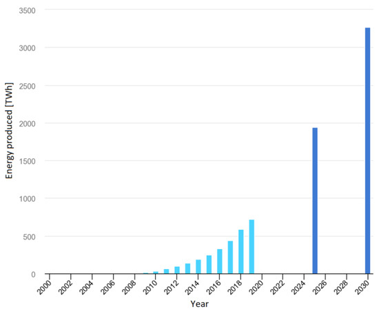
Figure 1. Solar photovoltaic generation: trend for 2000–2019 and targets for 2025 and 2030 [8] ©IEA 2020.

However, besides the contribution of solar PV power to solving the issue of global warming, there are negative aspects to this sudden rise. The main problem revolving around PV production is its high dependence on an intermittent natural resource—the sun. The production usually follows a specific very well-known trend, but it can be extremely volatile at times due to weather conditions. Solar PV production presents a problem for power system operation by itself, considering the effect of “the duck curve” that occurs due to the different peak times of PV and residential load. This issue is amplified when accounting for the unpredictability of production, leading to energy imbalance and increased cost of dispatching. Moreover, having a high percentage of uncontrollable and intermittent generation leads to a lower amount of spinning reserve by dispatched units. This yields the necessity for accurate forecasting methods to improve the economic efficiency, but most importantly, to assure the security and reliability of the power system operation. Furthermore, accurate forecast methods are paramount for producers and energy traders, since usually in the case of poor forecast penalties shall be paid to the market operator, reducing the net economic benefit. The large amount of PV installed as distributed generation on the distribution network has led to the need for an increased level of monitoring and controllability. This has been answered in the form of the deployment of smart grid components by modern distribution system operators (DSO), moving from the past fit and forget to a new fit and control approach for distributed generation. Mainly, this could increase the reliability of the medium voltage (MV) network, while also improving the hosting capacity and reducing losses through grid optimization techniques. Naturally, for all concerned actors, the importance and benefit from accurate forecast of PV production increases with the growth in installed capacity.

Such concepts are supported and developed within the InteGRIDy project [9], funded by the Horizon 2020 initiative, where the main goal is to advance the operation of the power system through improving the integration of RES, battery energy storage system (BESS) and e-mobility on 10 different pilot sites. Regarding the San Severino Marche pilot, the main scope is to develop an online MV grid optimization tool. Currently, there are 410 PV plants connected to the observed distribution network, which supplies a small town in the Central Italy, with installed powers ranging from 3 kW to 2.3 MW. Furthermore, 41 of them are directly connected to the MV network, while the rest are connected to the low voltage grid. Due to the large amount of solar PV installed power, PV forecast plays a crucial role in the optimization process. In collaboration with the DSO, data acquisition is centered around a database, where power and voltage measurement data for multiple devices are written with time resolution of 2 min, including nine of the PV plants.

The target of this paper is to cross-compare PV production forecast approaches in real-life conditions, to perform further optimization with respect to accuracy and computational complexity and, finally, quantify the performances of the chosen architecture for different time horizons. Regarding the structure of the paper, first an overview will be presented on forecasting methodologies and classifications, together with an overview on related works. Then, adopting a historic dataset, multiple forecasting techniques will be investigated given the parameters and data available for our implementation, with the goal of finding the most suitable one. Finally, further optimization of the selected methodology and the final implementation within an online forecasting procedure will be presented, together with selected accuracy metrics.

2. Forecasting Methods Classification and Related Works

In this paragraph, an in-depth overview on forecasting methods will be presented, together with a thorough overview on related works. In the literature, multiple classifications of solar PV forecast can be found, the first being related to the forecast horizon, or the amount of time between the time of forecasting and the time of prediction [10]. This factor is supposed to be crucial. i.e., the regulatory framework has to be properly evaluated in order to set up the algorithm coherently with the electric market rules. Multiple criterions exist, but according to [11] there are four types:

• Very short term—forecast horizon up to 6 h, usually performed with higher time resolutions.
• Short term—forecast horizon between 6 h and up to 3 days.
• Medium term—forecast horizon between 3 days and several months.
• Long term—forecast horizon between several months and multiple years.

Even though the forecasting error increases with the horizon observed, each type serves a different purpose; very short term prediction is useful for assuring the security of the power system in case of volatile weather conditions. Short term predictions have the widest implementation; they are used by producers and prosumers to optimize their profit, as well as for unit dispatching and load balancing. Medium term forecasts are mainly for asset management, whereas long term forecasts are used for analyzing resources and selecting future sites for deployment. Nowadays, the largest focus of the research is on short term forecast procedures, a relatively short window that allows for more accurate weather forecast and is directly related to the operation of the power grid, as well as the electricity markets.

According to the method used to perform the forecast, models can be classified as physical, statistical, or data-driven, and hybrid. Physical methods are based on numerical weather predictors (NWPs), sky imagery, and satellite imaging. Based on the area simulated, they can be either global or mesoscale, where it should be noted that for the purpose of PV forecast, only mesoscale with a resolution of up to 50 km should be used [12]. It is considered that forecasts for a group of distributed plants achieves better results when adopting an NWP due to the spatial averaging effect [13]. However, in order to decrease the spatial resolution and increase the accuracy, these complex algorithms use detailed meteorological data that have to be bought, increasing the costs for the utility in need of PV forecast. For this reason, they can be replaced by commercially available weather forecasting services, improving the economic efficiency, but limiting the accuracy and time resolution.

On the other hand, statistical methods rely on historical data and generally do not require any additional information regarding the physical characteristics of the PV plant, nor the location where it is installed. They include autoregressive moving average (ARMA) and autoregressive integrated moving average (ARIMA) modelling, as well as different types of machine learning techniques attempting to model the complex and nonlinear dependencies between input and output variables, including artificial neural networks (ANN), support vector machine (SVM), Markov chain, different tree and regression methods, persistence methods usually used as benchmark, etc. An improvement over the classical persistence method is the so called “smart persistence”. This method is detailed in [14], where instead of assuming continuity of irradiance or power output, it is considered that the sky clearness is constant and is combined with the clear sky model in order to obtain the irradiation. Furthermore, they can either be used to directly predict the power output, or indirectly by predicting weather parameters first. The latter concept is adopted in [15], comparing multiple naïve regression methods with machine learning techniques, with the goal of forecasting the solar irradiance. The optimal result was obtained by the least squares SVM, where it was found that using principal component analysis (PCA) to select the most important features to be used improved the accuracy by 9%. Moreover, a thorough overview on solar irradiation forecasting techniques is presented in [16], considering numerical weather predictor models, cloud imagery, and statistical methods.

The notion of reducing the dimensions of the input vector by analyzing the importance of each predictor in the dataset and excluding the ones that are weakly correlated to the output variable is extremely important for creating an accurate model. For example, the authors of [17] incorporated a preliminary stepwise regression to identify the importance of each predictors for the specific dataset before building the final prediction model. According to the literature, the weather parameters with the highest impact on PV production are solar irradiance, temperature, humidity, and rainfall [18,19,20].

ANNs are perhaps the most widespread statistical techniques, and according to many reviews, they are the most effective ones. This is due to the ability of the ANN to capture very detailed variations in the relationship between the input and output variables. Different types of ANNs are implemented in the literature for the purpose of direct or indirect PV forecast, including multi-layer perception (MLP), recurrent neural network (RNN), and feed-forward neural networks (FNN). Authors in [21] found that the accuracy of a properly optimized MLP ANN when predicting for a 24-h horizon was superior when compared with an ARIMA model, adaptive neuro-fuzzy model, and k-nearest neighbors model. Furthermore, in [22] the authors implement a RNN for a different application; mainly the goal was to predict the total daily production for an entire year, where the normalized root mean squared error (NRMSE) showed to be only 7%. The main drawbacks are related to the amount of data required, and the necessity for an accurate hyper-tuning of the model, including number of hidden layers, neurons etc. These values need to be optimized for each individual case.

On the other hand, tree-based methods usually do not depend as much on the model tuning and can obtain decent results even using default parameters [20,23]. An in-depth overview on the theoretic background on multiple tree methods, their implementation, comparison, and optimization is presented in [24]. A comprehensive analysis is performed in [25], where authors compared multiple techniques including binary regression trees, random forest (RF), gradient boosted regression trees for a horizon of 28–45 h. The best result was obtained by the RF model, obtaining an NRMSE between 10% and 12% for individual plants over 30-fold cross validation. The parameter tuning process of a RF is detailed in [23], and the performance is compared to a SVM. Adopting NRMSE as a metric, the results slightly favored the RF technique. The authors also found that when using large data sets, the accuracy of the model is improved when including the month, day, and hour as input.

The efficiency of adopting SVM as a PV forecaster was explored in multiple scientific works [19,23,26]. The performance of this technique depends on the selection of the kernel functions and the tuning of the parameters related to the kernel function. In the literature, the most frequently used kernel function for regression problems is the RBF (radial-basis function), since it is a nonlinear function which maps samples into a higher dimensional space, thus is easily able to handle nonlinear dependencies [27].

An alternative to using a statistical method to directly predict the output of the PV is adopting a physical representation of the PV system. In these cases, the plant is represented as a function of a set of independent variables, including the cell characteristics of the system [12]. Then, either an NWP or a statistical prediction of weather parameters can be used to obtain the output of the plant. However, it should be noted that this kind of forecast requires very specific details about the plant, such as location, panel tilt and orientation, inverter efficiency, etc.

These models offer limited accuracy when forecasting high time-resolution data, and for this reason are usually used to either predict the long-term behavior of production, or to predict an aggregated production over a longer period. For example, in [28] different types of ARIMA models are evaluated to predict the daily total energy production by a PV plant, using 1 year of historical production as the dependent variable.

This is due to the fact that the weather follows certain seasonal changes that are fairly easy to predict, and are observable from historic data, however when it comes to its dynamic behavior, NWPs offer much higher accuracy. Models that include a weather forecast, no matter if it is modeled separately or using a dedicated online weather forecast service, are usually referred to as hybrid or two-stage models. The authors of [21] implement such an approach, where a global NWP model is feeding input data for a localized meso-scale NWP, which is finally used as an input different types of statistical methods used to forecast daily energy production. These models are referred to as two-staged, with either adopting only a clear sky model of the location observed or including more advanced NWPs. The accuracy of these methods depends on the individual accuracy of the two models. Furthermore, in [29] the authors concluded that hybrid methods that use historical measurements of meteorological parameters for training machine learning algorithms usually lead to improved results. Indeed, this makes sense, since the input used to train the model is based solely on measurements, reducing the error with respect to training the algorithm with forecasted weather parameters. Another technique that is commonly used to improve accuracy is to cluster the dataset based on weather classification, thus creating multiple different models for different weather conditions. This, of course, is done at the expense of computational time and it requires larger datasets to assure that all different clusters are sufficiently present in the observed dataset. Then, the chosen model depends on the weather forecast, where the forecasted irradiation is compared against the clear sky model. In [12] the authors clustered the dataset into sunny and cloudy days, whereas the authors of [26] went a step further, classifying into four categories: sunny, cloudy, foggy, and rainy. Usually, the forecast is the most accurate for the sunny days, however, this can be attributed to the fact that the sunny cluster was the largest one, but also due to the accuracy of the weather forecast in poor weather conditions. Regardless, both [12,26] found improvements in the accuracy of the respective models when compared with considering only one large dataset.

However, in theory models that adopt a feature selection procedure are also considered ensemble methods. An overview of different feature selection methods combined with an ANN is presented in [30]. Similarly, in [31] the authors use a genetic algorithm to perform feature selection, where the most important features are then fed in an ANN. The authors found a 32% improvement with respect to the persistence method. The authors in [14] investigated using a smart persistence model as an input to a random forest algorithm and found improvements in the accuracy of the ensemble model.

Analyses performed in the literature offer some basic insight on the efficiency of each technique; however, the importance of different weather predictors and the efficiency of a selected model is dependent on each individual application, and thus the results vary from case to case. With respect to the application, most research efforts focus on the efficiency of the method itself and employ a larger dataset in order to perform the analysis, disregarding the time continuity of the data used to train the algorithms. However, a few authors focus on a real-life implementation, performing a mobile or an “online” forecast, where the goal is to periodically predict the hourly output of a PV output. For example, the authors of [32] employ an ANN to perform 24-h forecasts for a duration of 1 year, whereas in [33] the authors explore multiple auto-regressive methods combined with NWP parameters to forecast the output for a 24-h periods, but with a time horizon 12–36 h.

3. Methodology and Offline Validation

The goal of the analysis presented in this section is to find the most suitable method for PV forecast implementation within the InteGRIDy project. Taking into account the number of generators connected to the distribution network (as mentioned before, a few hundreds), it is hardly possible for the DSO to have access to detailed information about each power plant. For this reason, multiple different statistical techniques are investigated, detailed later in this section. It is important to clarify that in this section, the analysis is performed disregarding the time continuity of the forecast, but instead using the entire data set: i.e., the algorithm will be trained by using data that succeed the predicted output, data that of course would not be available in an online procedure. All these algorithms are in fact hybrid methods, utilizing both a statistical method, and a physical mesoscale model for the weather forecast, as well as an analytical clear sky irradiation model for the specific location. Multiple features related to weather parameters are used to train the models, with the dependent variable being the power output, since the goal is to directly predict the power injected in the grid by PV plants. Computations have been performed adopting the software package MATLAB [34].

3.1. Dataset

The analyses were performed using production data from one of the PV plants in the InteGRIDy project, with an installed power of 990 kW. The dataset represents a period of 142 days, between 28 February 2018 and 1 August 2018. Measurements were available with a time step of 1 min, but they were further sampled to an hourly rate. In some cases, data was either missing or corrupted; hours where more than 90% of the data is missing were disregarded from the dataset. Actually, the dataset being related to real-life power plants, data missing could be related to many different causes: fault in telecommunications, issues in the data logging, maintenance, etc. The preprocessed data available for the evaluation of the algorithms are presented on Figure 2.

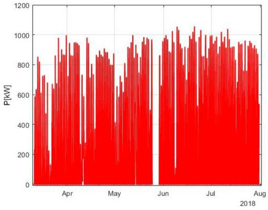
Figure 2. Power production profile.

The second part of the dataset is composed of weather parameters. Hourly weather forecasts for 100 different grid points are released by a commercial weather forecast provider [35] via a dedicated HTTP API service, as depicted in Figure 3. Parameters available in the forecast include global horizontal irradiance (GHI), temperature, humidity, wind speed, wind direction and precipitation. For the analyzed period in this chapter, forecasts were made available each day at midnight for the following 72 h. Thus, the accuracy for a power production forecasting procedure with a 24-h time horizon was evaluated.

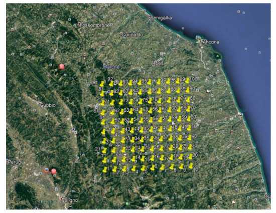
Figure 3. Grid points for the weather forecast.

A unique dataset was created considering only the hours for which both production and weather predictions were available. First, given the coordinates of the plant, the forecast that best suits the location was selected. Together with the production data vector, the dataset was composed by eight variables. The input vector was composed as:

• X1—clear sky GHI;
• X2—forecasted GHI;
• X3—temperature;
• X4—precipitation;
• X5—wind speed;
• X6—daily insulation;
• X7—hour of the day.

Feature X1 is the theoretical irradiation computed with the clear sky model, whereas features X2, X3, X4, and X5 are available from the weather forecast provider [36]. The clear sky irradiation was adopted for the specific location of the plant using the CAMS model, presented in [36]. On the other hand, predictor X6 was computed numerically, calculating the integral of the hourly forecasted GHI over the entire day. Data was further processed in a way that only hours where the clear sky GHI was higher than 0 were selected for further evaluation. The reason for this is twofold: we were interested in the accuracy of the algorithm during day hours when PV production is non-null, and, we were willing to avoid problems due to the heavily nonlinear dependency of the weather parameters and production during these periods; consequently the weather forecast and production during night hours were excluded from the dataset.

A clarification needs to be made that the analysis performed in this paper does not present an overall evaluation of the performance of each technique for PV forecast, but instead an evaluation of the performance of each method within our specific implementation, considering the data that is available for the forecasting procedure. Since actual measurements are only available for power production and not for weather parameters, the error of the production forecast will be affected by the accuracy of the commercially provided weather forecast. From the project’s point of view, the main goal is to optimize the total error, since due to lack of measurements for weather parameters on sites of the plants, it was not possible to evaluate the impact of the error introduced by the weather forecast provider.

3.2. Methods Investigated

3.2.1. Persistence

Persistence is the most straightforward statistical method, usually used as a benchmark for testing the accuracy of other approaches. In the case of solar PV, it assumes that the solar irradiance profile is periodical with a period of 24 h when observing limited amount of days, and remains more or less constant when observing relatively short periods. Additionally, in fact, research has shown that the accuracy drastically decreases as the time horizon of the forecast increases. This is true when observing the clear sky model, however, it is heavily constrained by the continuity of the actual weather conditions. This leads to the error of this model being with a large variance. The method can be described with the formula:

$$P_{out}\left(t\right)=P_{out}\left(t-\mathsf{\Delta }\right)$$

(1)

where $P_{out}$ is the output of the plant, whereas $∆$ in our case is 24 h, so for the implementation within this analysis, we adopted a D-1 approach.

3.2.2. Linear Regression

Linear regression is a linear approach for modeling the relationship between a scalar response and one or more explanatory variables. In the case of only one such variable, the method is called simple linear regression (SLR), depicted by the formula:

$$y=B_0+x\cdot B_1$$

(2)

where B₀ and B₁ are coefficients computed in order to fit the model with the available data. In the case of multiple parameters with linear dependence with the response variable, the model is called multiple linear regression (MLR) and presented as:

$$Y=B_0+{\left[X\right]}_{1\times m}\cdot {\left[B\right]}_{m\times 1}$$

(3)

where [B] is a vector made by coefficients that attempt to fit a linear model to the $m$ number of dependent features, while $\left[X\right]$ is the vector composed of those features. As previously mentioned, in the case of solar production forecast, the dominant variable is the solar irradiance, however the output of the plant is influenced in a heavily nonlinear way by other variables such as temperature, humidity, wind, etc.

In the analysis, two different SLRs are investigated: one as a function of the predicted GHI and the second as a function of the clear sky model. Moreover, the performance of a MLR adopting all seven features is evaluated. However, linear models become less accurate if the dependencies are not linear, which is the case with solar PV output. For this reason, the direction of the research was set towards machine learning algorithms that are able to incorporate strongly nonlinear dependencies and present a more accurate response.

3.2.3. Support Vector Machine

SVM is a supervised machine learning algorithm used for both, classification and regression. In the latter case, it is referred to as support vector regression. In the general case, the algorithm creates a hyperplane with N dimensions, where N is the number of features of the input dataset. This is done in a way that it optimally corresponds and fits the input data. Thus, the objective function is to minimize the l2 norm of the coefficient vector w, or in other words to make the hyperplane as flat as possible. Since in regression problems the output is a real number, a margin for tolerance must be set when obtaining the hyperplane. This margin is represented as the maximum error or tolerance—ε. Outliers being present in the data set can lead to underfitting of the algorithm, causing it to be too generalizing. To allow for some flexibility, SVM models have a cost parameter $C$, that controls the tradeoff between allowing training errors and forcing rigid margins. Increasing the value of $C$ increases the cost of samples that are not within the allowed error margin—${\mathsf{\xi }}_i$, forcing the creation of a more accurate model, which in return might not generalize well enough. This would lead to poor performances when testing the algorithm on a data set that had not been used in the training process. The objective function is defined as:

$$MIN\frac{1}{2}\Vert w\Vert +C{\displaystyle \sum }_{i=1}^N{\xi }_i$$

(4)

subject to the following constraint:

$$\left|y_i-w{x}_i-b\right|\le ϵ+\left|{\xi }_i\right|$$

(5)

For nonlinear dependencies such as in the case of PV forecast, kernel functions are introduced, transforming the dataset $X$ to a higher dimensional space, making the linear separation possible. In this case, the regression function of the hyperplane is given as:

$$Y=f\left(X\right)=⟨w,\phi \left(X\right)⟩+b$$

(6)

where $⟨°,°⟩$ represents a dot product, and $\phi \left(X\right)$ the transformation that maps the features into the higher dimension space. Three different kernel functions or transformations are considered in this preliminary analysis: gaussian or radial basis, polynomial, and linear. The specifics and the declaration of each kernel can be found in the following literature [37,38,39]. The algorithm can be optimized by adjusting its hyperparameters $C$, ε, and $\gamma$—kernel parameter. In this case, further optimization was not performed, and the following values suggested by the SVR documentation in MATLAB were adopted:

$$C=\frac{igr\left(Y\right)}{1.349}$$

(7)

$$ϵ=\frac{igr\left(Y\right)}{13.49}$$

(8)

where $igr\left(Y\right)$ represents the interquartile range or the difference between the 25th and the 75th percentile of the values in Y, which in our case is the power production vector. After further analysis, it was found that the values adopted are corresponding, in relative terms with respect to the rated power of the plant, to the results obtained in [23]. Furthermore, the authors in [23] found that the performance of the algorithm is not very sensitive to small variations in these hyperparameters.

3.2.4. Tree-Based Methods

Decision tree is a supervised machine learning algorithm, widely used for classification and regression problems. It works for both categorical and continuous input and output variables. Decision trees where the target variable can take continuous values, typically real numbers, are called regression trees. The tree building process is based on a top-down greedy approach, that is known as recursive binary splitting. In each node, a variable is used to split the tree in two branches, making sure that the chosen split has the lowest MSE, until no further improvement can be achieved. In the end, the terminal nodes are called leaves, a parameter that can be controlled by setting the minimum amount of allowed leaves. This is closely related to the variance of the output, and improper values can lead to over/underfitting. In our analysis, for all tree methods, a minimum of four leaves per tree was used. Still, this technique can result in a high variance of the output due to a small change in the training sample values [40]. To improve the performance of this techniques, usually ensemble methods such as boosting, and aggregating are adopted.

A typical example of boosting is the Adaptive Boosting (AdaBoost), a learning algorithm used to improve the performance of a simple classification tree. The algorithm uses multiple iterations to generate a single composite strong learner. AdaBoost creates a strong learner by iteratively adding weak learners. During each iteration, a new weak learner is added to the ensemble, and a weighting vector is adjusted to focus on samples that were misclassified in previous rounds.

Bootstrap aggregation or bagging is a general-purpose procedure for reducing the variance of a statistical learning method. Given a standard training set of size $N$, bagging generates $B$ new training sets $b^{th}$, each of size n, by sampling from the dataset uniformly and with replacement. By sampling with replacement, some observations may be repeated in each $b^{th}$ training set. This sample is known as a bootstrap sample. Then, the B models obtained are fitted using the above bootstrap samples and combined by either averaging the output for regression or voting for classification. In case of regression problems, the tree is trained on the $b^{th}$ bootstrapped training set to get the single prediction $f^{*b}$. Then, the aggregate prediction is evaluated as:

$$f_{bag}=\frac{1}{B}\cdot {\displaystyle \sum }_{b=1}^B{f}^{*b}$$

(9)

Even though bagging provides improvements over regular decision trees, it suffers from subtle drawbacks, such as increasing the computational complexity by $B$ times. Furthermore, since trees in the base are correlated, the prediction accuracy will get saturated.

Random forests (RF) provide an improvement over bagged trees by way of a small tweak that decorrelates the trees. Adopting this method, each tree is constructed using a random sample of predictors before splitting at each node. Since at the core random forests are also bagged trees, they lead to variance reduction as well. There are three main hyperparameters that need further optimization when adopting the random forests algorithm: leaf size, number of trees, and number of predictors sampled. A comprehensive sensitivity analysis was performed in [41], where it was found that the impact of the number of trees after reaching 50 was negligible. This was confirmed by repeating the analysis on our dataset, not showing any meaningful or steady improvement in accuracy. Similarly, the authors showed that algorithms with lower amount of leaves have a much better performance, a conclusion also reached in [42]. However, due to the negligible impact on computational time, we adopted an algorithm with 150 trees and four leaves. The random forest algorithm finds the predictors with higher correlation to the output variable and uses those predictors more frequently, thus improving the results. Generally, in case of $D$ predictors, choosing $D/3$ predictors per tree is a good choice for regression problems [43], thus the RF algorithm adopted in our case uses three features per tree.

3.2.5. Neural Networks

An artificial neural network (ANN) is composed of a large number of highly interconnected processing neurons utilizing different transfer functions, working in unison to solve specific problems. They are configured for individual applications, such as pattern recognition or data classification, through a learning process utilizing training datasets. In fact, after the learning process, they act as a black box in the eyes of the user, using an iterative procedure to act as a higher dimensional nonlinear function. Their main drawback is the abundancy of historical data required to train the algorithm even for simple tasks, as well as the necessity for hyperparameter tuning. This usually leads to relatively high computational times. A comprehensive overview and theoretic background of different ANN architectures for solar PV forecast can be found in the literature [44]; however, for the prediction performed in this analysis, the 24-h forecast is obtained adopting a multi-layer perception ANN with the following characteristics:

• Eight numerical predictors in input;
• One numerical output, power produced by the PV plant;
• Sigmoid activation function in the single neuron;
• Error back propagation with the Levenberg–Markquard algorithm for training;
• Mean square error (MSE) adopted as the error definition during the learning process.

Furthermore, a tuning process in the form of a sensitivity analysis was adopted to optimize the number of layers and neurons to use. The main observation is that the usage of a single neuron in the first layer has a large impact on performances. Considering the NRMSE and computational effort parameters, a local optimum was found adopting a configuration with nine neurons in the first layer and seven in the second, similarly to what was concluded in [45]. Moreover, an ensemble of 10 ANNs was adopted to improve the accuracy of the algorithm, as it has been shown in [45].

3.3. Validation and Performance Indices

The validation was performed adopting a 10-fold cross validation, where each method is trained with 90% of the dataset and tested with the other 10%. This was repeated for each part of the dataset in order to obtain more robust performance indices. An exception to this validation procedure is the case of the neural network, since it requires a validation set during the training process to avoid overfitting. In this case, the validation is a percentage extracted from the training set, while the test set remains only for the final evaluation of the performances.

The normalized values with respect to the maximum power measured of three different common performance indices in evaluating regression problems were considered: root mean squared error (RMSE), mean absolute error (MAE), and mean bias error (MBE), defined as:

$$NRMSE=\frac{100}{P_{max}}\sqrt{\frac{1}{N}}{\displaystyle \sum }_{i=1}^N{(P_i-\widehat{P_i})}^2$$

(10)

$$NMAE=\frac{100}{P_{max}\cdot N}{\displaystyle \sum }_{i=1}^N|P_i-\widehat{P_i}|$$

(11)

$$NMBE=\frac{100}{P_{max}\cdot N}{\displaystyle \sum }_{i=1}^N(P_i-\widehat{P_i})$$

(12)

where N is the number of samples, $P_i$ is the real output of the plant for sample $i$, and $\widehat{P_i}$ is the predicted value. In addition to these indices, the computational time for training the models and performing the prediction was evaluated and compared (data are related to an Intel i7—6700 at 3.4 GHz CPU with 16 Gb RAM).

3.4. Preliminary Results

The performances of each of the evaluated statistical methods are reported on Figure 4.

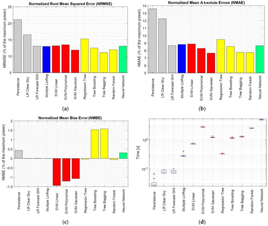
Figure 4. Evaluation of each proposed forecasting technique with respect to the following parameters (a) NRMSE (%)—with respect to Pmax; (b) NMAE (%)—with respect to Pmax; (c) NMBE (%)—with respect to Pmax; (d) computational time (s).

It can be seen that even a simple linear model can improve the performance with respect to the persistence model. In particular, it was found when the linear regression is based on the predicted GHI, the model is sufficiently accurate and has evidently better performance than some of the simpler machine learning techniques such as the regression tree. Adding more predictors which are not strongly correlated to the dependent variable does not have to improve the accuracy, as it can be seen comparing the error metrics of the SLR and MLR. Looking at the different kernels adopted for the SVM technique, expectedly the best performance can be seen by the Gaussian kernel, which is the most widely adopted. Observing the tree methods, tree bagging and RF show similar performances when considering RMSE and MAE, however the RF performs superiorly with respect to the MBE. Finally, the MLP neural network was found to have worse performance when compared to the Gaussian SVM and the RF techniques considering all error metrics. Usually, neural networks are used for much more complex problems, and for relatively simpler standard machine learning techniques have better performance.

Looking at the computational effort presented on Figure 4d, the execution time varies from milliseconds for the persistence, to tens of seconds for the neural networks, proving that neural networks are indeed the most computationally intensive method. These results were obtained by executing the calculations 10 times in order to get more robust values. The values presented depict the time required only to perform the prediction, so these values are strongly related to the complexity of each technique.

4. Real-Life Forecast Implementation

As it was previously mentioned, the final goal of this paper is to develop an accurate online forecasting procedure that feeds the grid optimization and real-time battery storage operation algorithms. The telecommunications network architecture that enables the power production data acquisition, as well as the challenges in reliability of data transfer within the InteGRIDy project are detailed in [46].

As of lately, the weather forecast data are available more frequently [36], each 6 h, for the same interval of 72 h. The weather forecast is downloaded each day at $t\forall t\in \left\{00:30,06:30,12:30,18:30\right\}$, and then saved in the project’s database. As a result, the mobile power production forecast is performed each 6 h, where for every 6 h period, 12 different weather forecasts are available, and thus, 12 different power production forecasts. Of course, both the grid optimization tool, as well as the real time operation of BESS, for each 6 h interval will consider only the most updated forecast. This is a time-dependent process, since data can only be acquired progressively. This means that for each forecast, a moving-window incremental dataset with a fixed size is used to train the algorithm. The metacode for the forecasting procedure that is executed 15 min after downloading the METEO forecast is depicted on Table 1.

Table 1. Mobile forecasting procedure.

Online Power Output Forecasting Procedure Flowchart

(a) Forecast the production of plants with available measurements For each of the nine plants with available real-time measurements: 1: Select the closest weather station based on latitude and longitude. 2: From the database, read the power production for the last $N$ training days, starting at the current day at 00:00. 3: Sample the data such as $P_t=\frac{1}{N}\ast {{\displaystyle \sum }}_{i=t-30\min }^{t+30\min }{P}_i$, where t is each hour from the training set. 4: Perform data scan to exclude any corrupted power measurements. An algorithm assuming linearity between the produced power and forecasted GHI is implemented. 5: From the database, for each hour read the latest available historical weather forecast from the weather station selected in step 1 for the last $N$ training days. 6: Synchronize the historical power production and weather forecast vector. 7: Train the algorithm adopting the synchronized vector of the dataset. 8: Using the weather forecast for the following 72 h and the trained model, forecast the power production output for the same period. 9: Save the forecasted data in the database (b) Calculate the average normalized power production forecast with respect to $Prated$, to be used by the algorithms for plants without available measurements. 1: For each hour $t$ of the 72-h interval$—P_{norm\left(t\right)}=\frac{1}{9}\ast {{\displaystyle \sum }}_{i=1}^9\frac{P_{forecast\left(i\right)}}{P_{rated\left(i\right)}}$. 2: Save the average normalized forecast in the project’s database.

4.1. Model Selection for the Mobile Forecast and Parameter Optimization

After the preliminary analysis investigating forecast techniques, see Section 3, a few methods showed similar results. However, when considering the online mobile implementation, the computational effort plays an important role in the decision, due to the fact that the forecast needs to be performed relatively often, for multiple power plants. Moreover, a large portion of the computational effort comes as a result of the communication between the forecasting software tool and the project’s database, as well as sampling and pre-scanning the data. In the preliminary simulations the entire data set was used to perform the analysis, which is something that would greatly increase the computational time. In the online forecast, the goal is to find the optimal training window that allows for accurate results, while respecting the time boundaries. For this reason, based on the results obtained in the preliminary analysis (see Section 3.3), random forests algorithms were selected as the most suited approach. In particular, the parameters that are optimized, together with the corresponding values investigated are:

• Training set size $\in$ {3 days, 7 days, 14 days, 21 days, 28 days, 35 days};
• Features used $\in$ {1, 2, 3, 4, 5};
• Number of trees $\in$ {25, 50, 150, 250}.

According to the analysis, analysis on the importance of the available features in the dataset, detailed in Section 3.1, the features were added in the following order:

• Forecasted solar GHI;
• Time vector—hour of the day;
• Clear sky GHI;
• Forecasted temperature;
• Forecasted humidity.

The optimization of the parameters was performed using the procedure depicted in Table 1 in an offline mode, where, in order to achieve common ground for different training set sizes, the errors were calculated on a common time interval between 1 February 2020 and 1 August 2020. Then, the performance in each case was evaluated adopting the NRMSE metric defined in Equation (10). The actual dataset used for training, of course, depends on the number of training days adopted. For the cases adopting 35 training days, data from the period between 26 December 2020 to 1 August 2020 were used. The analysis was performed, and the results of the optimization were verified using two plants with fairly diverse installed powers from the InteGRIDy project, with their power profiles being presented in Figure 4.

• Plant 1: Prated = 2300 kW; Pmax = 1974 kW.
• Plant 2: Prated = 100 kW; Pmax = 80.7 kW.

Figure 5 represents the power profiles of the respective power plants after the data scanning procedure mentioned in Table 1. As it was described, data can be missing from the dataset for short periods due to communication malfunction or other issues: in a real-life project this is a stressing factor that could strongly affect the forecast performances.

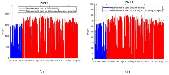
Figure 5. Power production used in the simulations. (a) Plant 1; (b) Plant 2.

4.2. Model Optimization Results

First, simulations were executed to observe the influence of the number of trees on the performance of the algorithm. It was found that adopting more than 50 ÷ 100 trees does not correlate with further improvement, but also that the effect on computational effort is negligible. Thus, a value of 150 trees was chosen, in order to reduce the dimension of the optimization process for the other two parameters. Then, an optimization procedure was performed for choosing the optimal training set size and the number of features used to train the RF algorithm, considering both the accuracy and the computational effort, the results of which can be found in Table 2, Table 3 and Table 4.

Table 2. NRMSE calculations for Plant 1.

	3 Days	7 Days	14 Days	21 Days	28 Days	35 Days
1 Feature	15.471	14.496	15.221	15.282	15.299	15.416
2 Features	14.934	13.379	13.099	12.824	12.848	12.914
3 Features	15.540	13.998	13.590	13.185	13.208	13.156
4 Features	15.722	13.905	13.517	13.065	13.036	13.061
5 Features	15.462	13.809	13.221	12.859	12.791	12.811

Table 3. NRMSE calculations for Plant 2.

	3 Days	7 Days	14 Days	21 Days	28 Days	35 Days
1 Feature	19.730	18.359	19.414	19.782	19.748	19.610
2 Features	17.664	15.160	14.620	14.340	14.364	14.402
3 Features	18.175	15.798	15.085	14.808	14.827	14.836
4 Features	18.406	16.020	15.299	14.851	14.679	14.699
5 Features	18.282	15.884	15.006	14.754	14.486	14.598

Table 4. Computational effort (s).

	3 Days	7 Days	14 Days	21 Days	28 Days	35 Days
1 Feature	2.51	3.19	4.79	5.80	11.24	12.16
2 Features	2.56	3.15	5.03	5.83	11.79	12.41
3 Features	2.49	3.10	5.02	5.73	11.45	12.27
4 Features	2.58	3.25	5.16	6.07	11.90	12.49
5 Features	2.54	3.18	5.11	6.01	12.02	12.38

First, the accuracy was evaluated adopting the NRMSE with respect to Pmax as error metric, detailed in Equation (10). These results, for Plant 1 and Plant 2, are displayed in Table 2 and Table 3, respectively. Having in mind that for each 6 h interval there are 12 different forecasts available, it should be noted that the accuracy evaluation presented in Table 2 and Table 3 was performed on the basis of the most recent forecast, which in fact is the one on the horizon between 1 and 6 h. The difference between the errors of the most recent forecast and the other 11 that are available is solely affected by the accuracy of the weather forecast considering different time horizons, and as such is constant for all different architectures that were investigated.

Analyzing the results presented in Table 2 and Table 3, it is evident that the trend of performance of different architectures is similar for the two plants. It can be seen that the highest accuracy is reached when adopting only two features: the forecasted solar GHI and the time vector. This can be explained by the weak correlation between temperature and humidity to the power output of the plant. Such machine learning algorithms need a larger amount of data to model these nonlinearities; however, in our case, the usage of large dataset is constrained by the computational effort. Moreover, the potential improvement brought by introducing the clear sky GHI for the specific location is highly dependent on the weather parameters. In case of sunny days, of course those values are very close to the actual irradiation. However, in case of cloudy and rainy days, it can be the cause of accuracy deterioration. From the results, it can be concluded that this is such a case.

Furthermore, the optimal architecture includes the adoption of 21 days worth of data to train the RF algorithm. In general, the performance of RF should increase when introducing larger datasets; nevertheless, in our implementation that is not the case because the algorithm is trained using forecasted values, so 1 day of heavily inaccurate weather forecast would corrupt the output for a larger amount of days.

The computational effort required for the various architectures of the RF algorithm is presented in Table 4. The values that are displayed are obtained as a mean value from the two plants, and represent the time required, in seconds, for one execution of the algorithm for one plant, including the computational effort required for the communication with the database.

Looking at Table 4, it can be concluded that the impact of the number of features on the total computational effort can be considered negligible. However, the amount of training data has a clear correlation to the computational effort, especially when adopting 28 and 35 training days. Considering the results obtained from these sensitivity analyses, the architecture consisting of 150 trees, 21 training days, and two features was selected as the best trade-off, and as such, is adopted in the online procedure described in Table 1.

4.3. Accuracy Analytics on the Architecture Adopted in the Project

In this section, some further error statistics on the adopted architecture are displayed. First, as it was described, for each 6 h period there are 12 different power output forecasts. In any case, the grid optimization tool will use the entire weather forecast, for the horizon between 1 and 72 h. Furthermore, in case the weather forecast is not available, real-time BESS operation tool would be forced to use older PV forecast. For these reasons, it is important to analyze the decrement in accuracy as the forecasting horizon increases. The results from this analysis are presented in Figure 6, with the NRMSE metrics already introduced in Equation (10). First, the results point to slightly lower accuracy for Plant 2 (the smaller one), something that was also noticeable from Table 2 and Table 3. However, it is clear that the trend of performance deterioration follows a very similar pattern throughout the different time horizons. The increment in NRMSE between the first and the last time horizon observed shows to be slightly more than 2%, a value which is very acceptable from our implementation’s point of view.

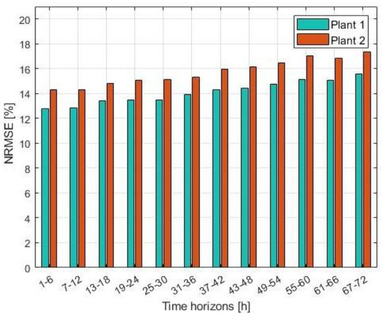
Figure 6. NRMSE with respect to Pmax for 12 different time horizons.

However, the RMSE does not provide much insight into the error distribution. For this reason, further analyses were performed to better understand this issue. First, a scatterplot of the absolute relative error as a function of the production is presented on Figure 7. The production on the y-axis is given in relative terms, with respect to Pmax, whereas the error is calculated with the equation depicted in Equation (13).

$$er{r}_{rel}=\frac{|P-\widehat{P}|}{P}$$

(13)

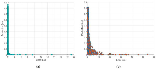
Figure 7. Absolute relative hourly error with respect to the production, as a function of the production. (a) Results for Plant 1; (b) results for Plant 2.

Looking at Equation (13) and Figure 6, first it can be seen that in general, the largest errors in terms of pu. occur mostly during lower production hours. Of course, this is mostly due to weather forecast overestimating the available GHI, and thus the actual production being significantly lower than expected for given hours of the evaluated period. Looking at the difference between the two plants, it can be seen that in the case of Plant 1, the accuracy is much more consistent, while in the case of Plant 2, it has a much higher variance and relatively high errors even for productions up to 0.3 pu.

The variance can also be seen looking at the boxplot of the absolute hourly error distribution, presented on Figure 8, where the same error from Equation (13) is adopted. Mainly, it can be observed that for the two plants, even though the mean value of the error is relatively low, it has a large variance, with a significant large number of outliers, which in this case are values outside of 1.5 times of the interquartile range of the error. This again points out to the significant influence of poor weather forecast on the variance of the forecasting error. Considering the results displayed on Figure 8, a possible solution could be to perform more rigorous scanning of the training dataset before each execution of the forecasting algorithm, with the goal of excluding not only corrupted data, but also data where the forecast has proved to be very inaccurate.

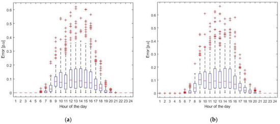
Figure 8. Boxplot of the absolute relative error for each hour of the day. (a) Results for Plant 1; (b) results for Plant 2.

All the results that were displayed so far have showed only the absolute value of the error. However, considering our implementation, it can be useful to understand if the sign of the error has a bias. Furthermore, it cannot be expected from the DSO to perform grid reconfiguration multiple times in a day, so the error of the total daily energy forecasted is an interesting metric to be considered. Thus, Figure 9 displays the probability density function (PDF) of the error in the daily energy forecast. The error is represented in a relative manner, with respect to the total energy actually produced, obtained with the equation presented in Equation (14).

$$er{r}_{day}=\frac{|E-\widehat{E}|}{E}$$

(14)

where E is the total energy produced and $\widehat{E}$ is the total energy forecasted for the day.

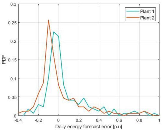
Figure 9. PDF of the daily energy relative forecast error, with respect to the energy produced.

Looking at Figure 9, it can be seen that both plants show bias toward the negative error values, whereas the error depicted by Plant 2 is significantly more biased. In our case, the fact that Plant 2 is relatively small leads to a smaller impact on the grid optimization algorithm, thus reducing the issue caused by this negative bias. These negative values actually suggest that in the most cases, the forecast overestimates the actual production, however these errors are not very significant. On the other hand, when the forecast underestimates the production, it does so with a higher error.

5. Conclusions

The work presented in this paper described an approach for the selection and implementation of a PV forecasting tool in a real-life scenario. Using an historic dataset with the same characteristics as the data available for the online approach, multiple statistical forecasting techniques were investigated, having found the random forest to be the best trade off. The procedure adopted by the online software module in charge of performing the online forecast was detailed. Two power plants within the InteGRIDy project, with fairly diverse rated powers, were used to validate the results. Throughout the analysis, it was found that even though the smaller plant showed slightly lower accuracy, the error metrics were following a very similar trend. Furthermore, it was found that the difference in the accuracy, considering NRMSE, of the forecast when considering different time horizons is very acceptable, mainly slightly above 2% when comparing the 6 h with the 72 h horizon. The accuracy was found to deteriorate almost linearly with increasing the time horizon, something that was expected as a result of the deterioration of the accuracy of the weather forecast. Furthermore, the error showed to be with significant variance, having a large number of statistical outliers. Finally, it was found that the forecasting procedure has a slight bias towards overestimating production, however, the amplitude of the error is lower, compared to the smaller amount of cases when the production is underestimated. Of course, this could be also influenced by the weather forecast itself. Considering the impact of the weather forecast on the accuracy of the forecasting procedure, a possible next step could be to perform more rigorous scanning of the training dataset before each execution of the forecasting algorithm, with the goal of excluding not only corrupted data, but also data where the forecast proved to be significantly inaccurate.

References

- Ourworldindata. Available online: https://ourworldindata.org/fossil-fuels (accessed on 15 August 2020).
- Ec Europa. Available online: https://ec.europa.eu/energy/sites/ener/files/documents/trends_to_2050_update_2013.pdf (accessed on 15 August 2020).
- UNFCCC—Kyoto Protocol. Available online: https://unfccc.int/kyoto_protocol (accessed on 15 August 2020).
- UNFCCC—Paris Agreement. Available online: https://unfccc.int/process-and-meetings/the-paris-agreement/the-paris-agreement (accessed on 15 August 2020).
- Ec Europa. Available online: https://ec.europa.eu/clima/policies/strategies/2020 (accessed on 17 August 2020).
- IRENA. Available online: https://irena.org/-/media/Files/IRENA/Agency/Publication/2020/Mar/IRENA_RE_Capacity_Highlights_2020.pdf?la=en&hash=B6BDF8C3306D271327729B9F9C9AF5F1274FE30B (accessed on 20 August 2020).
- IRENA. Available online: https://www.irena.org/costs (accessed on 20 August 2020).
- IEA. Available online: https://www.iea.org/data-and-statistics/charts/solar-pv-power-generation-in-the-sustainable-development-scenario-2000-2030 (accessed on 20 August 2020).
- InteGRIDy. Available online: http://www.integridy.eu/ (accessed on 20 August 2020).
- Antonanzas, J.; Osorio, N.; Escobar, R.; Urraca, R.; Martinez-de-Pison, F.J.; Antonanzas-Torres, F. Review of photovoltaic power forecasting. Solar Energy 2016, 136, 78–111. [Google Scholar] [CrossRef]
- Sreekumar, S.; Bhakar, R. Solar Power Prediction Models: Classification Based on Time Horizon, Input, Output and Application. In Proceedings of the International Conference on Inventive Research in Computing Applications, Coimbatore, India, 11–12 July 2018. [Google Scholar]
- Dolara, A.; Leva, S.; Manzolini, G. Comparison of different physical models for PV power output prediction. Solar Energy 2015, 119, 83–89. [Google Scholar] [CrossRef]
- Lorenz, E.; Hurka, J.; Heinemann, D.; Beyer, H.G. Irradiance Forecasting for the Power Prediction of Grid-connected Photovoltaic Systems. IEEE J. Sel. Top. Appl. Earth Obs. Remote Sens. 2009, 2, 2–10. [Google Scholar] [CrossRef]
- Tato, J.H.; Brito, M.C. Using Smart Persistence and Random Forests to Predict Photovoltaic Energy Production. Energies 2019, 12, 100. [Google Scholar] [CrossRef]
- Samanta, M.J.; Srikanth, B.K.; Yerrapragada, J.B. Short-Term Power Forecasting of Solar PVSystems Using Machine Learning Techniques. Available online: https://pdfs.semanticscholar.org/c1e5/7d5b888d8347dfc831c255bd1f374ee397a6.pdf (accessed on 1 July 2020).
- Diagne, M.; David, M.; Lauret, P.; Boland, J.; Schmutz, N. Review of solar irradiance forecasting methods and a proposition for small-scale insular grids. Renew. Sustain. Energy Rev. 2013, 27, 65–76. [Google Scholar]
- Ramsami, P.; Oree, V. A hybrid method for forecasting the energy output of photovoltaic systems. Energy Convers. Manag. 2015, 95, 406–413. [Google Scholar] [CrossRef]
- Lahouar, A.; Mejri, A.; Slama, J.B.H. Importance based selection method for day-ahead photovoltaic power forecast using random forests. In Proceedings of the International conference on Green Energy Conversion Systems, Hammamet, Tunisia, 23–25 March 2017. [Google Scholar]
- Wolff, B.; Kuhnert, J.; Lorenz, E.; Kramer, O.; Heinemann, D. Comparing support vector regression for PV power forecasting to a physical modeling approach using measurement, numerical weather prediction, and cloud motion data. Solar Energy 2016, 135, 197–208. [Google Scholar] [CrossRef]
- Abuella, M.; Chowdhury, B. Random forest ensemble of support vector regression models for solar power forecasting. In Proceedings of the IEEE Power & Energy Society Innovative Smart Grid Technologies Conference, Washington, DC, USA, 23–26 April 2017. [Google Scholar]
- Jimenez, L.A.F.; Jimenez, A.M.; Falces, A.; Vilena, M.M.; Garrido, E.G.; Santilian, P.M.L.; Alba, E.Z.; Santamaria, J.Z. Short-term power forecasting system for photovoltaic systems. Renew. Energy 2012, 44, 311–317. [Google Scholar] [CrossRef]
- Lee, D.; Kim, K. Reccurent Neural Network-Based Hourly Prediction of Photovoltaic Power Output Using Meteorological Information. Energies 2019, 12, 215. [Google Scholar] [CrossRef]
- Ahmad, M.W.; Mourshed, M.; Rezgui, Y. Tree-based ensemble methods for predicting PV power generation and their comparison with support vector regression. Energy 2018, 164, 465–474. [Google Scholar] [CrossRef]
- Geurts, P.; Ernst, D.; Wehenkel, L. Extremely randomized trees. Mach. Learn. 2006, 63, 3–42. [Google Scholar] [CrossRef]
- Zamo, M.; Mestre, O.; Arbogast, P.; Pannekoucke, O. A benchmark of statistical regression methods for short-term forecasting of photovoltaic electricity production, part I: Deterministic forecast of hourly production. Solar Energy 2014, 105, 792–803. [Google Scholar]
- Shi, J.; Lee, W.J.; Liu, Y.; Yang, Y.; Wang, P. Forecasting power output of photovoltaic system based on weather classification and support vector machine. In Proceedings of the IEEE Industry Applications Society Annual Meeting, Orlando, FL, USA, 9–13 October 2011. [Google Scholar]
- Dong, B.; Cao, C.; Lee, S.E. Applying support vector machines to predict building energy consumption in tropical region. Energy Build. 2005, 37, 545–553. [Google Scholar] [CrossRef]
- Atique, S.; Noureen, S.; Roy, V.; Subburaj, V.; Bayne, S.; Macfie, J. Forecasting of total daily solar energy generation using ARIMA: A case study. In Proceedings of the 2019 IEEE 9th Annual Computing and Communication Workshop and Conference, Las Vegas, NV, USA, 7–9 January 2019. [Google Scholar]
- Monteiro, C.; Jimenez, L.A.F.; Rosado, I.J.R.; Jimenez, A.M.; Santilan, P.M.L. Short-term Forecasting Models for Photovoltaic Plants: Analytical versus Soft-Computing Techniques. Math. Probl. Eng. 2013, 2013, 1–9. [Google Scholar] [CrossRef]
- Raza, M.Q.; Nadarajah, M.; Ekanayake, C. On recent advances in PV output power forecast. Solar Energy 2016, 136, 125–144. [Google Scholar] [CrossRef]
- Pedro, H.T.C.; Coimbra, C.F.M. Assessment of forecasting techniques for solar power production with no exogenous inputs. Solar Energy 2012, 86, 2017–2028. [Google Scholar] [CrossRef]
- Chen, C.; Duan, S.; Cai, T.; Liu, B. Online 24-h solar power forecasting based on weather type classification using artificial neural network. Solar Energy 2011, 85, 2856–2870. [Google Scholar] [CrossRef]
- Bacher, P.; Madsen, H.; Nielsen, H.A. Online short-term solar power forecasting. Solar Energy 2009, 10, 1772–1783. [Google Scholar] [CrossRef]
- MATLAB. Available online: https://www.mathworks.com/products/matlab.html (accessed on 10 January 2018).
- DataMeteo. Available online: www.Datameteo.com (accessed on 11 March 2018).
- Soda-PRO. Available online: http://www.soda-pro.com/documents/10157/326332/CAMS72_2015SC3_D72.1.3.1_2018_UserGuide_v1_201812.pdf/95ca8325-71f6-49ea-b5a6-8ae4557242bd (accessed on 1 February 2020).
- Abuella, M.; Chowdhury, B. Solar Power Forecasting Using Support Vector Regression. In Proceedings of the American Society for Engineering Management International Annual Conference, Charlotte, NC, USA, 26–29 October 2016. [Google Scholar]
- Saedsayad. Available online: https://www.saedsayad.com/support_vector_machine_reg.htm (accessed on 3 August 2020).
- Hastie, T.; Tibshirani, R.; Friedman, J. Kernel Smoothing Methods. In The Elements of Statistical Learning, 2nd ed.; Springer: New York, NY, USA, 2009; pp. 191–216. [Google Scholar]
- Ahmad, M.W.; Mourshed, M.; Rezgui, Y. Trees vs. neurons: Comparison between random forest and ANN for high-resolution prediction of building energy consumption. Energy Build. 2017, 147, 77–89. [Google Scholar] [CrossRef]
- Ibrahim, I.A.; Khatib, T.; Mohamed, A.; Elmenreich, W. Modeling of the output current of a photovoltaic grid-connected system using random forest technique. Energy Explor. Exploit. 2017, 36, 132–148. [Google Scholar] [CrossRef]
- TowardsDataScience. Available online: https://towardsdatascience.com/optimizing-hyperparameters-in-random-forest-classification-ec7741f9d3f6 (accessed on 10 August 2020).
- Hastie, T.; Tibshirani, R.; Friedman, J. Boosting and Additive Trees. In The Elements of Statistical Learning, 2nd ed.; Springer: New York, NY, USA, 2009; pp. 337–384. [Google Scholar]
- Kashyap, Y.; Bansal, A.; Sao, A.K. Solar radiation forecasting with multiple parameters neural networks. Renew. Sustain. Energy Rev. 2015, 49, 825–835. [Google Scholar] [CrossRef]
- Dolara, A.; Grimaccia, F.; Leva, S.; Musseta, M. A Physical Hybrid Artificial Network for Short Term Forecasting of PV Plant Power Output. Energies 2015, 8, 1138–1153. [Google Scholar] [CrossRef]
- Falabretti, D.; Moncecchi, M.; Mirbagheri, M.; Bovera, F.; Fiori, M.; Merlo, M.; Delfanti, M. San Severino Marche Smart Grid Pilot within the InteGRIDy project. Energy Procedia 2018, 155, 431–442. [Google Scholar] [CrossRef]
© 2020 by the authors. Licensee MDPI, Basel, Switzerland. This article is an open access article distributed under the terms and conditions of the Creative Commons Attribution (CC BY) license (http://creativecommons.org/licenses/by/4.0/).