Abstract
An impeller blade with a slot structure can affect the velocity distribution in the impeller flow passage of the centrifugal pump, thus affecting the pump’s performance. Various slot structure geometric parameter combinations were tested in this study to explore this relationship: slot position p, slot width b1, slot deflection angle β, and slot depth h with (3–4) levels were selected for each factor on an L16 orthogonal test table. The results show that b1 and h are the major factors influencing pump performance under low and rated flow conditions, while p is the major influencing factor under the large flow condition. The slot structure close to the front edge of the impeller blade can change the low-pressure region of the suction inlet of the impeller flow passage, thus improving the fluid velocity distribution in the impeller. Optimal slot parameter combinations according to the actual machining precision may include a small slot width b1, slot depth h of ¼ b, slot deflection angle β of 45°–60°, and slot position p close to the front edge of the blade at 20–40%.
1. Introduction
The pumps are classified as general machinery with varied applications [1,2,3,4,5]. Blade slotting was first used in the aviation industry to improve the separation of airflow over the wings [6]. Blade slotting technologies work by allowing the pressure difference to be adjusted between two sides of an airfoil so that gas on the high-pressure side flows through the slot, thus forming a jet upon reaching the low-pressure side. This jet effectively delays the separation of the boundary layer of the airfoil surface and increases the airfoil head coefficient to improve overall airfoil properties [7,8,9]. The effects of various slot parameters on the performance of blade centrifugal pump represent significant information for engineers.
Many scholars have investigated the effects of slotting technology on the mechanical performance of impellers. Tang et al. [10], for example, carried out a numerical simulation using the three-dimensional (3D) uncompressible Navier–Stokes equation to determine the influence of the slot position and slot width on the centrifugal fan performance. They found that the efficiency and total pressure of the slotted impeller improved under the design conditions; noise was also reduced as the performance under non-design conditions improved. Huang et al. [11] optimized slotting long and short blade impeller parameters based 3D, incompressible Navier–Stokes equations and a k-ꞷ turbulence model followed by a prototype test; they concluded that the slotting technique improves blower performance. Wang et al. [12] used the RNG k-ε model to simulate the multiphase flow in a centrifugal pump with a slotted blade structure. They found that an opening near the blade inlet improves the cavitation performance of the medium-low specific speed centrifugal pump. Ye [13] studied the effects of slotted blades on the centrifugal efficiency, head, and internal flow field of a pump; the blade slot was found to increase the head and flow of the pump under high flow conditions. Gao et al. [14] determined the loss of pressure and coefficient of heat transfer in the slotted turbine blade of a trailing edge by numerical simulation and experimental verification; they also analyzed the effects of slotting on the flow and heat transfer characteristics of the surface. Xing [15] studied the effects of long and short blades on the internal flow field and impeller performance of pumps using the numerical simulation method. Yuan [16] found that the use of splitter blades effectively improves the performance of low specific speed centrifugal pumps. Kergourlay et al. [17] used the unsteady Reynolds average Navier–Stokes (URANS) method to study the effect of blade slotting on the flow field in a centrifugal pump. An impeller with a slotted structure was found to make the circumferential speed and pressure distribution more uniform while slightly improving the pump performance. Gölcü et al. [18] found that a slotted-blade impeller is less loaded than the impeller without a slotted blade.
There has been a great deal of research on slotting the blades of low specific speed centrifugal pumps [12,13,19], but previously published techniques have certain limitations due to the sole analysis of a single condition. In an effort to systematically explore the effects of slotted blades on the performance of centrifugal pumps, the present study was conducted to test four parameters: slotted blade position, slotting width, slotting angle, and slotting depth. The effects of various combinations of different parameters on the performance of medium specific speed centrifugal pumps were explored accordingly via orthogonal design.
2. Numerical Simulation Method
2.1. Computation Model
A medium specific speed centrifugal pump with a speed ratio of ns = 85 was selected to study the effects of blade slotting on the pump performance. The specific speed is formulated as follows:
where, n is the rotating speed (r/min), Q is the rated point flow rate (m3/s), and H is the rated point head (m).
The main design parameters of the pump are shown in Table 1.

Table 1.
Main design parameters of centrifugal pump.
The total flow field was computed to consider the effects of ring clearance leakage on the pump’s performance. As shown in Figure 1, the computational domains in this case include the inlet section, impeller, pump cavity, volute, and outlet section, wherein the pump cavity portion includes the front and ring cavities. The extension lengths of the inlet and outlet sections in the computational domain were set to four times the diameters of the inlet and outlet pipes, respectively, to ensure a sufficient flow development.
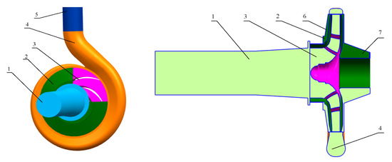
Figure 1.
Simulation pump model. 1. Inlet section; 2. pump cavity; 3. impeller; 4. volute; 5. outlet section; 6. front cavity and 7. rear cavity.
2.2. Meshing
Commercial ANSYS-ICEM17.0 software was utilized to mesh various computational domains. As the structured meshes only contained quadrilaterals or hexahedrons in this case, their topological structure was equivalent to a uniformly orthogonal mesh within a rectangular domain. Accordingly, the nodes on each layer of the mesh lines can be effectively adjusted to ensure a high quality [20,21,22,23,24]. The overall computational domain was structured and meshed and the boundary layer of the meshes in the vicinity of the near wall of the blade was refined. The quality of meshes within all computational domains was above 0.35 (Figure 2).
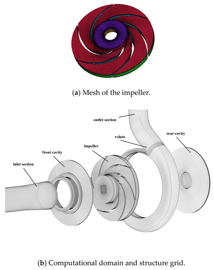
Figure 2.
Mesh of the pump.
The efficiency, head, and power of the rated point of the pump were considered indexes for mesh independence verification of the unslotted centrifugal pump model. The global maximum mesh size was used to control the mesh density of each computational domain. Local meshes within each computational domain were specifically refined to ensure the desired mesh quality. The meshing results are shown in Table 2.
Table 2.
Analysis of the grid independent.
Figure 3 shows the effects of the number of meshes in different cases on the head, power, and efficiency of the simulated pump. A numerical calculation on a mesh with a global mesh size of 2 mm was conducted with both the computational cycle and computational accuracy taken into account.
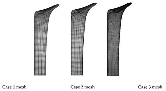
Figure 3.
Schematic diagram of the blade structure grid.
2.3. Computational Cases and Boundary Conditions
Numerical calculations were performed in ANSYS-CFX19.2 software (ANSYS CFX. 19.2″ ANSYS CFX 19.2 Documentation. 2019). The turbulence model in this case was a standard k-ω turbulence model. The computational impeller domain was set to a rotational domain and all other computational domains were set to static. Data transfer at the interface between the static domains and the rotational domains was achieved by the frozen rotor method.
To consider the effects of the impeller cover plate on the flow, all other inner wall surfaces within the pump cavity excluding those in contact with the impeller outlet surface were set to a rotational wall surface. The roughness of each computational domain surface was set to 10 μm to observe the effects of the material on the internal flow characteristics of the pump. The boundary conditions were set to pressure inlet and mass outflow. The reference pressure was set to a standard atmospheric pressure, the wall surface was placed under a non-slip boundary condition, and a standard wall surface function was used with the convergence accuracy set to 10−4.
2.4. Orthogonal Design of Blade Slots
To explore the effects of blade-slotting on the medium specific speed pump systematically, four factors including the slotting position, slotting width, slotting depth, and slotting angles of the blades were studied via the orthogonal design method. The orthogonal design method is a scientific design technique wherein test plans are reasonably arranged to determine the main factors that influence certain indexes within a brief testing time [25]. Many researchers have used orthogonal designs to study the performance of centrifugal pumps [26,27,28,29]. Considering the time and cost burdens of the test, the geometrical factors of the slots as they affect pump performance were observed in this study by combining CFD technology with an orthogonal design.
2.5. Determining the Test Factors
As discussed above, four sets of geometric parameters were taken as test factors: slot position p slot width b1, slot deflection angle β and slot depth h (Figure 4). Slot position p is the position of the slot on the blade. Based on the arc length of the blade profile, four uniform levels were taken from the inlet edge of the blade to the outlet edge of the blade: 20%p, 40%p, 60%p, and 80%p. Three levels of the slot width b1 were selected: 0.5 mm, 1 mm, and 1.5 mm. As shown in Figure 4, the angle β is the included angle between the slot and the tangent line of the blade in the slot position. The deflection angle of the slot relates to the effects of the slot jet on the liquid flow in the flow passage. Three angles were tested: 30°, 45°, and 60°. The slot depth h is the axial distance from the inner surface of the front cover plate, relative to the blade outlet width b. Three depths were selected: 1/4 b, 2/4 b, and 3/4 b.
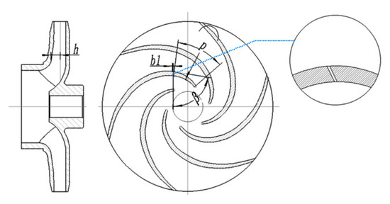
Figure 4.
The schematic diagram of the gap geometry parameters.
As shown in Table 3, the L16 orthogonal table was selected for these four factors.
Table 3.
Factor level table.
3. Analysis of Numerical Simulation Results
3.1. Test Verification
To validate the numerical simulation method used in this study, the original model was tested. As shown in Figure 5, the test rig is an open-type system, which is composed of two parts, namely, the data acquisition system and the water circulation system. The DN100 electromagnetic flowmeter whose maximum allowable error is ±0.5% was used to measure the flow rate Q. The valve of the pump inlet pipeline was fully opened during the test and the flow condition points were collected through the pump outlet pipeline valve. To secure a smooth external characteristic curve during the collection process, recording was performed at an interval of 5 m3/h from the shutoff point to the large flow condition point for a total of 17 operating points.
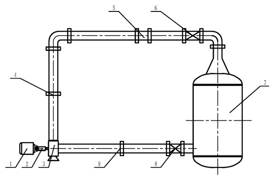
Figure 5.
Schematic diagram of the test rig. 1. Motor; 2. torque meter; 3. centrifugal pump; 4. outlet pipeline pressure section; 5. DN100 electromagnetic flowmeter; 6. outlet pipeline valve; 7. water tank; 8. inlet pipeline valve and 9. inlet pipeline pressure section.
Table 4 shows the pump performance test results. As the rotational speed of the pump was not constant at 2850 r/min during actual operation, for an effective comparison against the numerical calculation results, the external characteristic data of the pump was converted to a rated speed of 2850 r/min according to the rules of similarity theory.
Table 4.
Pump performance test results.
Figure 6 shows a comparison between the test-based and simulated pump performance indicators. To completely reflect the external characteristic variation curve from the shutoff point to the maximum flow condition during the pump test, eight flow condition points were simulated from 0.1Q to 1.4Q. The numerical simulation results accurately predicted the external characteristic curve of the pump within the whole range of operating conditions as observed in the test. The relative errors in the head, efficiency, and power of the rated operating points were 4.4%, 2.95%, and 4%, respectively. All were smaller than 5%, which indicates that the numerical simulation method was accurate. Further, these results suggest that the orthogonal design case accurately reflects slotting effects numerically.
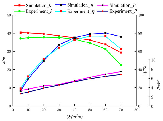
Figure 6.
Comparison of test and numerical results.
3.2. Direct Analysis of Orthogonal Design Case
Sixteen sets of orthogonal design cases were used in this study. Prototyping all of them would be costly and time-consuming, so considering the accuracy of the numerical calculation method, the full flow field numerical simulation method was selected as the research tool for this orthogonal design. To observe the effects of slotting on the performance of the medium specific speed centrifugal pump, full flow field numerical simulations were conducted at four operating condition points: 0.6Q, 0.8Q, 1.0Q, 1.2Q, and 1.4Q for 16 sets of slotted impellers in conjunction with the volutes.
This study centers on the effects of different slotting cases on pump performance. Table 5, Table 6 and Table 7 show the numerical simulation results of 0.6Q, 1.0Q, and 1.4Q, respectively. The orthogonal test data was processed to assess the main factors influencing the pump head and efficiency in the slotted blade case [18]. The range analysis method was used to observe the effects of the levels of the factors at 0.6Q, 1.0Q, and 1.4Q operating conditions on the pump’s performance.
Table 5.
0.6Q numerical simulation results.
Table 6.
1.0Q numerical simulation results.
Table 7.
1.4Q numerical simulation results.
In the case of a greater range, different levels of a given factor lead to a larger amplitude of variations in the test indicators. To this effect, the factor corresponding to the maximum range was the most important factor. Ki(i = 1,2,3,4) denotes the sum of the tests of the same level in any of the columns in Table 3, where i corresponds to different levels of the same factor, ki = Ki/n denotes the arithmetic mean value of different levels of the same factor, n denotes the number of occurrence of the same level in any of the columns in the table, and R = max(k1, k2, k3, k4) − min(k1, k2, k3, k4) denotes the range. A range analysis of 0.6Q are shown in Table 8 and Table 9.
Table 8.
0.6Q head analysis.
Table 9.
0.6Q efficiency analysis.
The primary and secondary geometric parameters of slots influencing the pump performance at 0.6Q were obtained as shown in Table 10.
Table 10.
The order of influence of the gap geometry parameters on pump performance at 0.6Q.
Table 11.
1.0Q head analysis.
Table 12.
1.0Q efficiency analysis.
The primary and secondary geometric parameters of slots influencing the pump performance at 1.0Q were obtained as shown in Table 13.
Table 13.
The order of influence of the gap geometry parameters on pump performance at 1.0Q.
Table 14.
1.4Q head analysis.
Table 15.
1.4Q efficiency analysis.
The primary and secondary geometric parameters of slots influencing the pump performance at 1.4Q were obtained as shown in Table 16.
Table 16.
The order of influence of the gap geometry parameters on pump performance at 1.4Q.
Range analyses of the operating condition points, 0.6Q, 1.0Q, and 1.4Q indicated that the slot width and depth under the small flow conditions and rated conditions have the greatest effects on the pump head and efficiency among the parameters tested. The slot position appeared to have little effect on the performance of the pump under small flow conditions. In the case of large flow conditions, however, the slot position had a greater effect on pump performance than any other parameter.
To analyze the effects of the changes in factor levels on the pump performance more intuitively, a trend variation chart was plotted with the head and efficiency of the pump as indicators. As shown in Figure 7, the head h0.6Q was the largest when the blade slotting position p was close to the outlet side and the slot deflection angle β was the smallest under the small flow condition 0.6Q. The head h0.6Q decreased progressively as slot width b1 and the slot depth h increased, and an inflection point emerged on the curve of the head h0.6Q as slot position p varied. Based on the steepness of the curve variation trend, the primary and secondary factors influencing the head h0.6Q were slot width b1, slot deflection angle β, slot depth h, and slot position p, respectively. This result was consistent with the range analysis results. The efficiency η0.6Q also increased as b1 and h decreased. The efficiency η0.6Q curve trend also presented an inflection point with the changes in the slot position. Based on the trend graph, in order of intensity, the factors influencing the efficiency η0.6Q were slot depth h, slot width b1, slot deflection angle β, and slot position p.
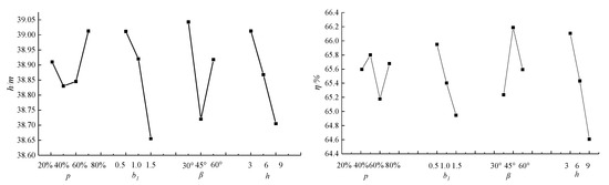
Figure 7.
0.6Q head (left) and efficiency (right)-factor relationship.
As shown in Figure 8 and Figure 9, under the conditions of 1.0Q and 1.4Q, the heads of h1.0Q and h1.4Q were the largest when the blade slot position p was in the vicinity of the inlet edge of the blade. Like 0.6Q, the heads of h1.0Q and h1.4Q and the efficiencies of η1.0Q and η1.4Q decreased progressively as slot width b1 and the slot depth h increased. h1.0Q, h1.4Q, η1.0Q, and η1.4Q also increased progressively as slot deflection angle β increased.
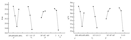
Figure 8.
1.0Q head (left) and efficiency (right)-factor relationship.
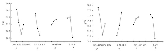
Figure 9.
1.4Q head (left) and efficiency (right)-factor relationship.
3.3. Analysis of Internal Flow Field
The orthogonal test results suggest that blade slotting improved the head at small flow condition points and the efficiency at large flow condition points, which is consistent with previously published results. Under the working condition of 0.6Q, the head of Case 1 was 39.3 m; in the original case the head was 38.5 m. The head and efficiency in Case 1 for the 1.4Q condition were 30.15 m and 77.86%, respectively, and in the original case were 30.05 m and 77.09%. To further explore the effects of the geometric slot parameters on pump performance, the distributions of performance curves of the original model and Case 1 were compared as shown in Figure 10.
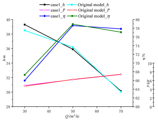
Figure 10.
Comparison of case 1 and original model.
Figure 11 and Figure 12 show cloud diagrams of the static pressure distribution of the blade unfolding at the section of the pump impeller flow passage (the section value Span was 0.9) in the original model and Case 1 of slotted blades under the conditions of 0.6Q and 1.4Q, respectively. As shown in Figure 11, under the 0.6Q condition, the static pressure distributions of the blade unfolding in Case 1 and the original model differed significantly. The distribution of pressure in the impeller flow passage from the blade inlet to the outlet was characterized by a low-pressure region in the first half-section of the impeller flow passage and a high-pressure region in the second half-section of the passage. The pressure gradient in the second half-section of the impeller flow passage was large because the flow passage diffusion was severe, which might have created a secondary back flow at the outlet of the impeller under small flow conditions. This is also likely a cause of the low efficiency of the medium-low specific speed centrifugal pump at the small flow condition point.
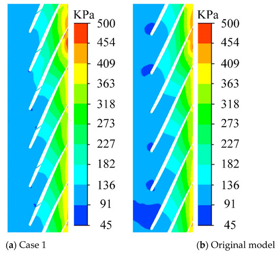
Figure 11.
Static pressure distributions on the cross section of the impeller channel at 0.6Q.
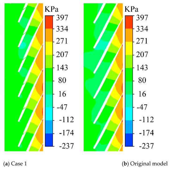
Figure 12.
Static pressure distributions on the cross section of the impeller channel at 1.4Q.
A significant low-pressure region was also observed in the position close to the inlet edge of the original model. Due to slotting in the position close to the inlet edge of the impeller, the distribution of blade unfolding static pressure disappears in the low-pressure region close to the inlet position of the blade in Case 1 and the pressure distribution is significantly more uniform than that in the original model. Vortexes and back flows are unlikely to form in the inlet position of the blade in this case, which is also one of the reasons why the head of the model in Case 1 is larger than that of the original model under the 0.6Q condition.
Under the 1.4Q large-flow condition, the diagram for the blade unfolding static pressure distribution in the case of the original model was similar to that in Case 1, however, the original model had a significant low-pressure region with considerable variations in the pressure gradient in the first half-section of the impeller flow passage inlet. This is mainly because the fluid flow angle of the incoming liquid increases with the flow rate while the inlet setting angle of the blade remains unchanged. As a result, the inlet setting angle is smaller than the liquid flow angle; a flow cutoff forms at the working surface in the position of the blade inlet creating a low-pressure region. Similarly, the changes in pressure gradient in the static pressure distribution diagram of blade unfolding in Case 1 are smaller than those of the original model due to the fact that the blade is slotted near the inlet.
As shown in Figure 13, the pressure distribution is shown on the blade surface at the mean circumferential flow surface. Under 0.6Q, the pressure distribution of the original model and the Case 1 model were quite different (Figure 13). At the position near the inlet side, the pressure of the pressure surface and the suction surface of the Case 1 model were larger than the original model. This further illustrates that the Case 1 model improved the pressure distribution at the inlet edge of the blade due to slotting. The pressure near the inlet edge of the blade was higher than that of the original model under the 1.4Q large-flow condition.
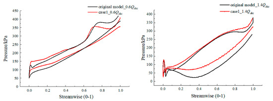
Figure 13.
Variation of the blade load with streamwise at 0.6Q (left) and at 1.4Q (right).
Figure 14 and Figure 15 show the distribution of pressure clouds in the middle plane of the blade flow channel. The pressure gradient distribution of the Case 1 model is more uniform than the original model under the 0.6Q condition (Figure 14); the original model shows a lower pressure than the Case 1 model near the blade inlet as well, which is consistent with the findings shown in Figure 11 and Figure 12. The enlarged view in the figure shows where, due to the existence of a gap, the local low-pressure gradient distribution was more uniform in the original model. This gap jet made the streamline in the inlet low-pressure area closer to the profile of the blade airfoil, thereby improving the local flow field. Figure 15 shows that under the large flow rate of 1.4Q, the impact of the gap on the local area was relatively small. The local enlarged view did not show similar phenomena to the small flow conditions. Generally speaking, the gap improved the local flow field under small flow conditions.
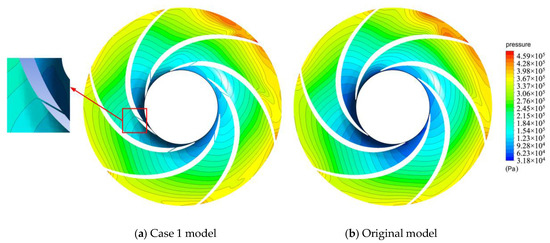
Figure 14.
Static pressure distribution in the middle plane of the blade flow channel at 0.6Q.
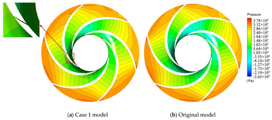
Figure 15.
Static pressure distribution in the middle plane of the blade flow channel at 1.4Q.
Figure 16 shows a diagram of the relative velocity distribution under the 1.4Q operating condition in the impeller calculation domain. This distribution was normal; the average velocity of the impeller calculation domain was basically 11 m/s. The velocity distribution amplitude of velocity in Case 1 was larger than that of the original model, which indicates that the velocity within the impeller was concentrated near the desired value and was uniform throughout the impeller calculation domain. This was also one of the reasons why the efficiency and head of Case 1 were larger than those of the original model.
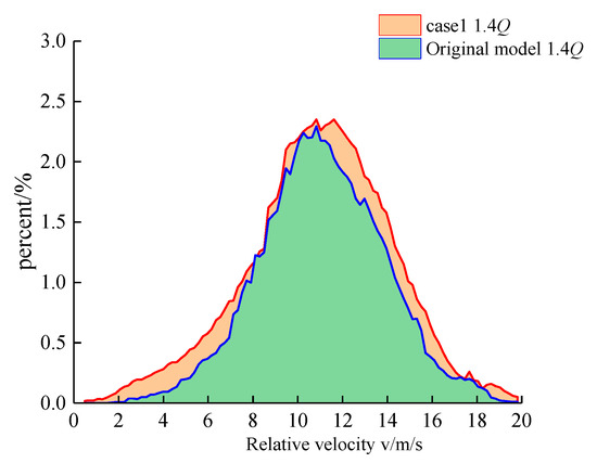
Figure 16.
Velocity distribution in the impeller calculation domain at 1.4Q.
4. Conclusions
(1) Orthogonal test results show that various geometrical slot parameters affected pump performance. Under small flow conditions, the factors most intensely influencing the pump head were slot width b1 > slot deflection angle β > slot depth h > slot position p. The factors most intensely influencing the pump efficiency were slot depth h > slot width b1 > slot deflection angle β > slot position p. The main factors influencing the pump head and efficiency under rated flow conditions were slot width b1 and slot depth h, whereas the main factor influencing the pump head and efficiency under large flow conditions was slot position p.
(2) The orthogonal test results also indicate that under low flow conditions and rated flow conditions, the head and efficiency of the pump decreased as blade slot width increased. These effects were linear.
(3) Different combinations of slot geometric parameters in Case 1 were found to increase the pump head at the small flow condition point as well as the efficiency and head of the pump at the large flow condition point compared to the original model without slots. The internal flow field shows that slotting near the front edge of the blade improved the low-pressure region of the impeller inlet flow passage and brought the flow velocity distribution in the impeller field under the large flow conditions closer to the desired value as the flow velocity distribution grew more uniform.
(4) To improve the performance of the pump, optimal slot parameter combinations according to the actual machining precision might include a small slot width b1, slot depth h of ¼ b, slot deflection angle β of 45–60°, and slot position p close to the front edge of the blade at 20–40%.
Author Contributions
C.W. performed the writing—reviewing and editing; H.W. made the investing; B.L. performed the data curation; C.H. made the software; L.L. made the methodology. All authors have read and agreed to the published version of the manuscript.
Funding
This work was supported by the National Natural Science Foundation of China (Grant No. 51609105), Changzhou Sci&Tech Program (Grant No. CJ20190048), Jiangsu Province Graduate Practice Innovation Project (Grant No. SJCX18_0743).
Acknowledgments
In this section you can acknowledge any support given that is not covered by the author contribution or funding sections. This may include administrative and technical support, or donations in kind (e.g., materials used for experiments).
Conflicts of Interest
The authors declare no conflict of interest.
References
- Li, X.; Chen, B.; Luo, X.; Zhu, Z. Effects of flow pattern on hydraulic performance and energy conversion characterisation in a centrifugal pump. Renew. Energy 2020. [Google Scholar] [CrossRef]
- Li, X.; Shen, T.; Li, P.; Guo, X.; Zhu, Z. Extended compressible thermal cavitation model for the numerical simulation of cryogenic cavitating flow. Int. J. Hydrog. Energy 2020. [Google Scholar] [CrossRef]
- Shi, L.; Zhang, W.; Jiao, H.; Tang, F.; Wang, L.; Sun, D.; Shi, W. Numerical simulation and experimental study on the comparison of the hydraulic characteristics of an axial-flow pump and a full tubular pump. Renew. Energy 2020, 153, 1455–1464. [Google Scholar] [CrossRef]
- Wang, C.; Chen, X.; Qiu, N.; Zhu, Y.; Shi, W. Numerical and experimental study on the pressure fluctuation, vibration, and noise of multistage pump with radial diffuser. J. Braz. Soc. Mech. Sci. Eng. 2018, 40, 481. [Google Scholar] [CrossRef]
- Shi, L.; Zhu, J.; Tang, F.; Wang, C. Multi-Disciplinary Optimization Design of Axial-Flow Pump Impellers Based on the Approximation Model. Energies 2020, 13, 779. [Google Scholar] [CrossRef]
- Ni, P.; Wu, G.; Wang, Y.; Gao, Y. The application of slotted blade. Mech. Des. Manuf. 2014, 3, 90–92. [Google Scholar]
- Li, J.; Tian, H.; Niu, Z. Study on the flow fields in a centrifugal fan with slots along the blade ends. J. Eng. Thermophys. 2009, 30, 2028–2030. [Google Scholar]
- Wang, Y.; Mei, Y.; Liu, B.; Cao, Z. Numerical approach for turbine blade with trailing edge ejection. J. Propuls. Technol. 2002, 23, 315–317. [Google Scholar]
- Wang, Y.; Liu, B.; Jiang, J.; Chen, Y. Experiment and numerical simulation investigation of turbine blade with trailing edge ejection. J. Aerosp. Power 2006, 21, 474–479. [Google Scholar]
- Tang, X.; Huang, D.; Zhu, Z. Application of boundary layer control technology in centrifugal impeller. Fluid Mach. 1998, 9, 15–19. [Google Scholar]
- Huang, D.; Bian, X.; Tang, X.; Lu, Y. Application of slotted technique on splitter blade in centrifugal fan. J. Tsinghua Univ. (Sci. Technol.) 1999, 39, 6–9. [Google Scholar]
- Wang, Y.; Xie, S.; Wang, W. Numerical simulation of cavitation performance of low specific speed centrifugal pump with slotted blades. J. Drain. Irrig. Mach. Eng. 2016, 34, 210–215. [Google Scholar]
- Ye, D. Research on the Performance of Centrifugal Pump with Slotted Blades; Jiangsu University: Zhenjiang, China, 2013. [Google Scholar]
- Gao, Y.; Yan, X.; Li, J. Investigation on characteristics of flow and heat transfer in a turbine blade with trailing-Edge cutback. J. Xi’an Jiaotong Univ. 2018, 52, 31–40. [Google Scholar]
- Xing, G. Numerical Study on the Flow Field inside a Centrifugal Impeller with Slotted Blade; Chongqing University: Chongqing, China, 2008. [Google Scholar]
- Yuan, S. Advances in hydraulic design of centrifugal pumps. In Proceedings of the 1997 ASME Fluids Engineering Division Summer Meeting, Vancouver, BC, Canada, 22–26 June 1997; pp. 1–15. [Google Scholar]
- Kergourlay, G.; Younsi, M.; Bakir, F.; Rey, R. Influence of splitter blades on the flow field of a centrifugal pump: Test-analysis comparison. Int. J. Rotating Mach. 2007, 2007, 1–13. [Google Scholar] [CrossRef]
- Gölcü, M.; Pancar, Y. Investigation of performance characteristics in a pump impeller with low blade discharge angle. World Pumps 2005, 468, 32–40. [Google Scholar] [CrossRef]
- Yuan, J.; Li, S.; Fu, Y. Splitter blades’ effect on characteristics of centrifugal pump by orthogonal experiment. Drain. Irrig. Mach. 2009, 27, 306–309. [Google Scholar]
- Uzol, O.; Camci, C. Aerodynamic loss characteristics of a turbine blade with trailing edge coolant ejection: Part2 External aerodynamics, Total pressure losses and predictions. ASME J. Turbomach. 2001, 123, 249–257. [Google Scholar] [CrossRef]
- Yousefi, H.; Noorollahi, Y.; Tahani, M.; Fahimi, R.; Saremian, S. Numerical simulation for obtaining optimal impeller’s blade parameters of a centrifugal pump for high-viscosity fluid pumping. Sustain. Energy Technol. Assess. 2019, 34, 16–26. [Google Scholar] [CrossRef]
- He, X.; Zhang, Y.; Wang, C.; Zhang, C.; Cheng, L.; Chen, K.; Hu, B. Influence of critical wall roughness on the performance of double-channel sewage pump. Energies 2020, 13, 464. [Google Scholar] [CrossRef]
- Wang, H.; Long, B.; Yang, Y.; Xiao, Y.; Wang, C. Modelling the influence of inlet angle change on the performance of submersible well pumps. Int. J. Simul. Model. 2020, 19, 100–111. [Google Scholar] [CrossRef]
- Wang, C.; Shi, W.; Wang, X.; Jiang, X.; Yang, Y.; Li, W.; Zhou, L. Optimal design of multistage centrifugal pump based on the combined energy loss model and computational fluid dynamics. Appl. Energy 2017, 187, 10–26. [Google Scholar] [CrossRef]
- Li, Y.; Hu, C. Experimental Design and Data Processing; Chemical Industry Press: Beijing, China, 2008. [Google Scholar]
- Shi, W.; Zhou, L.; Lu, W.; Zhang, L.; Wang, C. Orthogonal test and optimization design of high-head deep-well centrifugal pump. J. Jiangsu Univ. (Nat. Sci. Ed.) 2011, 32, 400–404. [Google Scholar]
- Wang, H.; Shi, W.; Lu, W.; Zhou, L.; Wang, C. Optimization design of deep well pump based on latin square test. Trans. Chin. Soc. Agric. Eng. 2010, 41, 56–63. [Google Scholar]
- Yuan, S.; Zhang, J.; Yuan, J.; FU, Y. Orthogonal experimental study effect of main geometry factors of splitter blades on pump performance. Drain. Irrig. Mach. 2008, 26, 1–5. [Google Scholar]
- Zhang, J.; Zhu, H.; Li, Y.; Yang, C. Optimization design of hybrid pump impeller based on orthogonal design method. J. China Univ. Pet. (Ed. Nat. Sci.) 2009, 33, 105–110. [Google Scholar]


© 2020 by the authors. Licensee MDPI, Basel, Switzerland. This article is an open access article distributed under the terms and conditions of the Creative Commons Attribution (CC BY) license (http://creativecommons.org/licenses/by/4.0/).