A Finite Mixture GARCH Approach with EM Algorithm for Energy Forecasting Applications

Abstract

Enhancing forecasting performance in terms of both the expected mean value and variance has been a critical challenging issue for energy industry. In this paper, the novel methodology of finite mixture Generalized AutoRegressive Conditional Heteroskedasticity (GARCH) approach with Expectation–Maximization (EM) algorithm is introduced. The applicability of this methodology is comprehensively evaluated for the forecasting of energy related time series including wind speed, wind power generation, and electricity price. Its forecasting performances are evaluated by various criteria, and also compared with those of the conventional AutoRegressive Moving-Average (ARMA) model and the less conventional ARMA-GARCH model. It is found that the proposed mixture GARCH model outperforms the other two models in terms of volatility modeling for all the energy related time series considered. This is proven to be statistically significant because the p-values of likelihood ratio test are less than 0.0001. On the other hand, in terms of estimations of mean wind speed, mean wind power output, and mean electricity price, no significant improvement from the proposed model is obtained. The results indicate that the proposed finite mixture GARCH model is a viable approach for mitigating the associated risk in energy related predictions thanks to the reduced errors on volatility modeling.

1. Background

1.1. Introduction

Volatility prediction is a major consideration for energy-related processes or variables, which include, but are not limited to, oil prices, energy consumptions, electricity prices, energy generations from traditional and renewable sources, and meteorological variables such as wind speed. In recent years, renewable energy has become increasingly cost-competitive [1]. In terms of levelized cost of generating electricity, the median costs of solar PV and onshore wind generations are lower than those of gas and coal generations in the United States, China, Europe, and India. Most notably, the generation of wind energy continued to grow in 2019 and 2020 despite the COVID-19 pandemic caused challenges [2,3]. As such, the volatility prediction of renewable energy processes becomes increasingly important in that it can mitigate the challenges stemming from the supply of intermittent power to market and thus facilitate the healthy and sustainable development of renewable energy [4].

In the prediction process of many energy variables, one usually considers two aspects: the expectation (mean) and the variance. Take wind speed forecasting as an example: wind farms need not only the accurate mean wind speed, but also the turbulence (variance) of wind speed in order to effectively manage the operations with less risk. The expectation answers the question of “what is likely to happen?”, while the variance could be explained as “how much risk is associated?” A good understanding of this “risk” is critical to appropriately managing the energy conversion systems, such as preparing for suitable production plans and scheduling proactive maintenance. Also, factoring in the “risk” can provide invincible advantages for active participants of energy exchange market to develop effective electricity price bidding strategies.

In this paper, we propose a novel two-component approach for forecasting means and variance of energy time series data. The approach involves finite mixture Generalized AutoRegressive Conditional Heteroskedasticity (GARCH) models with the adoption of Expectation–Maximization (EM) algorithm for model parameter estimation. The approach adopts the general autoregressive–moving-average (ARMA) model and combines it with the mixed normal GARCH (MN-GARCH) model. To comprehensively evaluate the effectiveness of the proposed approach, three energy related subjects are selected, namely, wind speed, wind power generation, and electricity price. For each case, we develop the finite mixture GARCH models with the help of EM algorithm and compare their prediction performances with those of the traditional ARMA and ARMA-GARCH models. The main contributions of this research lie in two aspects: (1) the innovative approach of combining finite mixture GARCH and EM algorithm is for the first time proposed such that non-normal distributions could be handled and the parameter estimation could be processed efficiently; and (2) the proposed method is found to be superior in terms of volatility modeling compared with the traditional GARCH models based on the comprehensive evaluation of three types of energy time series data. As such, the proposed approach is a general methodology that should be applicable to both renewable and non-renewable sectors.

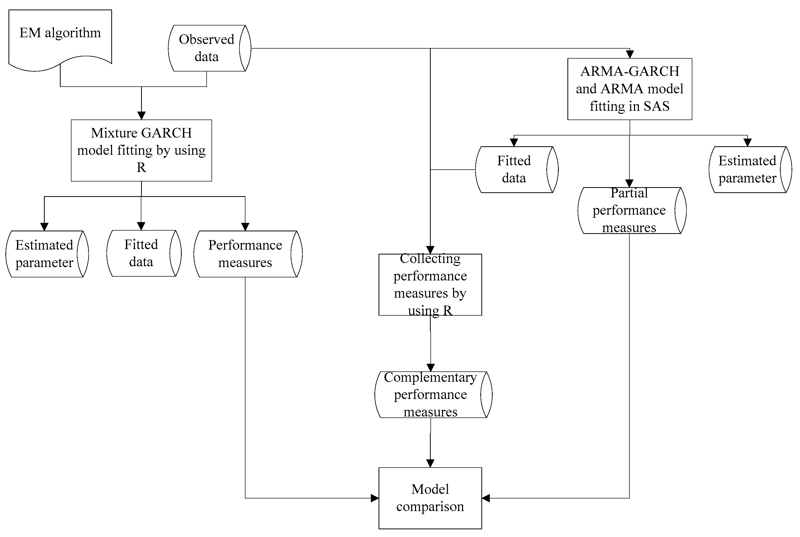
The remaining sections are organized as follows. In Section 1.2, a brief literature review is provided regarding energy time series modeling and prediction, along with a critical analysis. In Section 2, the principles of general finite mixture model and the EM algorithm, as well as the necessary formulations are briefly introduced. In Section 3, we present the implementation procedure of the finite mixture GARCH approach with EM algorithm, and describe the framework. In Section 4, the proposed approach is for the first time tested on wind speed, power generation, and electricity price data. The results are analyzed and compared against the ARMA and ARMA-GARCH models. Finally, conclusions are drawn in Section 5.

1.2. Brief Literature Review

There are many data-driven approaches for modeling and predicting energy related variables, such as statistical models, neural networks, generalized impulse response analysis methods, and hybrid approaches [5,6,7,8,9]. These approaches are usually for mean prediction. Meanwhile, the generalized autoregressive conditional heteroscedastic (GARCH) models have been developed to model the non-constant-volatility/heteroskedasticity [10]. The heteroskedasticity generally implies that different time series observations have non-constant variance. However, in the commonly used ordinary least square (OLS) estimation, the presence of heteroskedasticity becomes a challenge because OLS estimation assumes constant variances. In this case, GARCH method becomes a promising tool to deal with time series data with time varying volatility. For various purposes, GARCH models have been extended into different forms, such as nonlinear GARCH (NGARCH), exponential GARCH (EGARCH), and the GARCH-in-mean (GARCH-M) model [11,12,13,14,15]. GARCH model applications have appeared in various areas. In particular, the popularity of GARCH models has been increasing in energy related studies. For instance, Garcia et al. [16] propose a GARCH model for electricity prices. The results can be further used to develop bidding strategies or negotiation skills in the electricity market. Liu et al. [17] develop an approach to estimate the wind power generation by modeling wind speed volatility and thus the operation probability of wind turbines. The proposed approach is valuable not only for the management of wind farms, but also for the integration of wind energy in the electricity market. Sun et al. [18] adopt ARMA-GARCH models for forecasting of solar radiation, and show that the ARMA-GARCH models can outperform other forecasting models without the consideration of volatility.

However, GARCH models cannot properly handle the data with heavy tailed or asymmetric distributions (e.g., non-normal distributions). To address this, the finite mixture GARCH approach has been developed, and it has received much attention from academia and industry in recent years. The original concept of finite mixture model was proposed for two normal probability density functions [19]. However, it is until last two decades before that this methodology was adopted in serious applications due to the tremendous advancement of computing power [20]. To date, the existing studies for finite mixture GARCH models are concentrated in financial related areas. Tang et al. [21] indicate that the finite mixture ARMA-GARCH model is more effective than either the mixture of AR models or AR-GARCH models. Hossain and Nasser [22] compare the performance of finite mixture ARMA-GARCH with those of neural network and support-vector machines (SVM) approaches for financial time series. The results indicate that the finite mixture ARMA-GARCH model outperforms the other two methods in terms of directional symmetry (DS) and weighted directional symmetry (WDS). Haas et al. [23] propose a MN-GARCH model for the daily return data on a stock index. The empirical analysis suggests good performance of the MN-GARCH model for both in-sample fit and out-of-sample forecasting. Similarly, Alexander and Lazar [24] apply the general normal mixture GARCH(1,1) for exchange rate modeling. The preliminary results reveal that the two-component mixture GARCH(1,1) model outperforms the mixture models with three or more components, as well as the symmetric and skewed student’s GARCH models. Broda et al. [25] propose an approach that combines GARCH model with the mixtures of Paretian distributions. The approach is then applied to model seven major FX and equity indices, and it turns out to be more effective than the traditional GARCH-type models. Besides, other significant works include the mixture asymmetric GARCH model for option pricing [26], and a class of mixture GARCH model for capturing volatility and periodicity in non-linear time series data [27].

Although the mixture GARCH models are effective modeling tools for time series data, the major drawback is the existence of large number of parameters, which renders the process of model fitting rather difficult. One way for effectively estimating parameters in finite mixture models could be the expectation–maximization (EM) algorithm. Usually, the EM algorithm is comprised of two steps, namely, the expectation step (E-step) and the maximization step (M-step). The E-step provides the expectation on the missing information based on the conditional distribution of observations, while the M-step provides the maximum likelihood estimates (MLE) to the parameters based on the observations and expectation of the missing information. There are numerous applications of the EM algorithm, and particularly significant efforts have been made to fit the Gaussian mixture models by using various versions of EM algorithms [28,29,30,31]. The well-known drawbacks of EM algorithm lie in the local convergence and initialization, but recent studies have addressed the problem by combining new techniques, such as k-means, greedy learning, unsupervised learning, and genetic algorithm, with the EM algorithm [32,33,34,35].

The mixture GARCH model is also able to be fitted with the EM algorithm. However, the related studies are relatively scarce. Nikolaev et al. [36] use the EM algorithm and mixture GARCH model for estimating the volatility of financial returns, where AR(1) is applied for mean equation and Student’s t distribution is used as the component for the mixture model. Cheng et al. [37] combine the normal mixture GARCH model with the EM algorithm for S&P500 Index and Hang Seng Index forecasting, where AR(1) is also assumed for the mean equation. In addition, Wu and Lee [38] apply the EM algorithm and the normal mixture GARCH model to study the excess market returns, where no mean equation is considered. Tang et al. [21] extend the mixture AR-GARCH model to ARMA-GARCH model, which is fitted with EM algorithm and applied for the stock price forecasting. However, the mean equation is also considered as a mixture component, and this arrangement is lack of support from the mixture GARCH theory.

Although the literature shows potentials for financial applications of finite mixture GARCH models, the effort for adopting the methodology on energy related subjects has been lacking. More importantly, the combination of finite mixture GARCH approach with EM algorithm has not been attempted to the best of our knowledge. As such, the proposed research helps to bridge the research gap.

2. Finite Mixture GARCH Model and EM Algorithm

2.1. Foundation of GARCH Model

It is well known that GARCH approach is effective for modeling the time varying volatility. It was first developed by Bollerslev [10] as an extension for ARCH model. Consider the error term ${\epsilon }_t$ from ARMA(p, q) model,

$$y_t={\displaystyle \sum }_{i=1}^p{a}_i{y}_{t-i}+{\displaystyle \sum }_{j=1}^q{b}_j{\epsilon }_{t-j}+{\epsilon }_t$$

(1)

where $a_i$, $i=1,\cdots p$ and $b_j$, $j=1,\cdots q$ are the coefficients for the auto regressive and moving average terms, respectively. Similarly, $p$ and $q$ are the orders of autoregressive and moving average terms, respectively. If the error term ${\epsilon }_t$ has a time varying variance, it can be modeled as,

$${\epsilon }_t=\sqrt{v_t}{z}_t$$

(2)

where $z_t$ is a white noise process with mean 0 and variance 1, and can be formulated by the following equation,

$$v_t={\alpha }_0+{\displaystyle \sum }_{i=1}^P{\alpha }_i{v}_{t-i}+{\displaystyle \sum }_{j=1}^Q{\beta }_j{\epsilon }_{t-j}^2$$

(3)

where ${\alpha }_0$ is a constant term, ${\alpha }_i$, $i=1,\cdots P$ and ${\beta }_j$, $j=1,\cdots Q$ are the coefficients for the GARCH and ARCH terms, respectively. Similarly, $P$ and $Q$ are the orders of GARCH and ARCH terms, respectively. In this way, the error term follows the GARCH process of order $P$ and $Q$, denoted as GARCH(P, Q). When $P=0$, the current conditional variance is not dependent upon the previous conditional variance, and this means that the GARCH model degenerates into an ARCH model.

2.2. Gaussian Mixture Model

A Gaussian mixture model is a weighted mixture of finite Gaussian component densities. Assume that a random variable $X$ follows Gaussian/Normal Mixture (NM) distribution with $k$ components, i.e., $X~NM\left(w_1,\cdots w_k;{\mu }_1,\cdots {\mu }_k;{\sigma }_1^2,\cdots {\sigma }_k^2\right)$, the probability density function of $X$ is,

$$f\left(x\right)={\displaystyle \sum }_{i=1}^k{w}_i{\varphi }_i\left(x\right)$$

(4)

where $w_i$ is the weight for the ith Gaussian component with $w_i\in \left(0, 1\right)$ and ${\displaystyle \sum }_{i=1}^k{w}_i=1$, ${\varphi }_i\left(x\right)$ is the probability density function of the ith Gaussian component represented as ${\varphi }_i\left(x\right)=\varphi \left(x;{\mu }_i,{\sigma }_i^2\right)$, and ${\mu }_i$ and ${\sigma }_i^2$ are the mean and variance for the corresponding Gaussian distribution.

2.3. Finite Mixture GARCH Model

The finite mixture GARCH model borrows the idea of both GARCH model and Gaussian mixture model. Given the error term ${\epsilon }_t$ from ARMA(p, q) model, the finite mixture GARCH model assumes that ${\epsilon }_t$ follows a Gaussian mixture distribution, i.e., ${\epsilon }_t~NM(w_1,\cdots w_K;{\mu }_{t,1},\cdots {\mu }_{t,K};{\sigma }_{t,1}^2,\cdots {\sigma }_{t,K}^2)$, where $w_k$ is the weight for the kth Gaussian component with $w_k\in \left(0, 1\right)$ and ${\displaystyle \sum }_{k=1}^K{w}_k=1$. Moreover, the concept borrowed from GARCH model implies that the variance of the kth component ${\sigma }_{t,k}^2$ can be formulated as follows,

$$\begin{gathered} {\sigma }_{t,k}^2={\alpha }_{0,k}+{{\displaystyle \sum }}_{i=1}^P{\alpha }_{i,k}{\sigma }_{t-i,k}^2+{{\displaystyle \sum }}_{j=1}^Q{\beta }_{j,k}{\epsilon }_{t-j}^2, \\ \mathrm{for}k=1,\cdots K \end{gathered}$$

(5)

where ${\alpha }_{0,k}$ is a constant term, ${\alpha }_{i,k}$, $i=1,\cdots P$ and ${\beta }_{j,k}$, $j=1,\cdots Q$ are the coefficient for the GARCH and ARCH terms, respectively. Similarly, $P$ and $Q$ are the orders of GARCH and ARCH terms, respectively. Hence, by combining the above mentioned technology, the finite mixture GARCH(P, Q) can be formulated as follows,

$$y_t={\displaystyle \sum }_{i=1}^p{a}_i{y}_{t-i}+{\displaystyle \sum }_{j=1}^q{b}_j{\epsilon }_{t-j}+{\epsilon }_t,$$

(6)

$${\widehat{y}}_t={\displaystyle \sum }_{i=1}^p{a}_i{y}_{t-i}+{\displaystyle \sum }_{j=1}^q{b}_j{\epsilon }_{t-j}$$

(7)

$$p\left(y_t\right)={\displaystyle \sum }_{k=1}^K{w}_k{G}_{}\left(y_t,{\widehat{y}}_t,{\sigma }_{t,k}^2\right)$$

(8)

$${\sigma }_{t,k}^2={\alpha }_{0,k}+{\displaystyle \sum }_{i=1}^P{\alpha }_{i,k}{\sigma }_{t-i,k}^2+{\displaystyle \sum }_{j=1}^Q{\beta }_{j,k}{\epsilon }_{t-j}^2$$

(9)

where $p\left(y_t\right)$ is the probability density function of $y_t$, and ${\sigma }_{t,k}^2$ is the variance of the kth component at time t.

2.4. EM Algorithm for Estimating Parameters in Finite Mixture GARCH Models

As mentioned previously, in this study we adopt the EM algorithm to find parameters of finite mixture GARCH models that maximize the log-likelihood function. The joint probability of the finite mixture GARCH model is

$$p\left(y\right)={\displaystyle \prod }_{t=1}^T{\displaystyle \sum }_{k=1}^K{w}_k{G}_{}\left(y_t,{\widehat{y}}_t,{\sigma }_{t,k}^2\right)$$

(10)

and the optimal parameters that maximize the log-likelihood function need to be found,

$$\widehat{\theta }=arg\underset{\theta }{max}lnp\left(\mathit{y}\right)$$

(11)

where $\theta$ represents the set of parameters in the model.

The two steps of EM algorithm, namely, E-step and M-step, are described below for the finite mixture GARCH model fitting.

• E-step

Let $\mathit{Z}={\left\{Z_t\right\}}_{t=1}^T$ be the unobserved information, and we define $Z_t=k$. If $y_t$ is produced by the kth component of the model, we have the following equations

$$p\left(\mathit{y},\mathit{Z}\right)={\displaystyle \prod }_{t=1}^{T}p(y_t|Z_t)p(Z_t)$$

(12)

$$p\left(Z_t=k\right)=w_k$$

(13)

Given the information above, the complete information joint distribution is

$$p\left(\mathit{y},\mathit{Z}\right)={\displaystyle \prod }_{t=1}^{T}p(y_t|Z_t)p(Z_t)$$

(14)

and the corresponding log-likelihood function

$$lnp\left(\mathit{y},\mathit{Z}\right)={\displaystyle \sum }_{t=1}^{T}lnp\left(y_t|Z_t\right)p\left(Z_t\right)$$

(15)

Hence, the Q function of the EM algorithm will be

$$\begin{array}{l}Q\left(\mathit{\theta },{\mathit{\theta }}^{*}\right)\\ =E_{Z|y,{\mathit{\theta }}^{*}}\left\{{\displaystyle {\displaystyle \sum }_{t=1}^T}lnp\left(y_t|Z_t\right)p\left(Z_t\right)\right\}\\ ={\displaystyle {\displaystyle \sum }_{Z_1=1}^K}\cdots {\displaystyle {\displaystyle \sum }_{Z_T=1}^K}\left\{{\displaystyle {\displaystyle \sum }_{t=1}^T}ln[p(y_t|Z_t)p\left(Z_t\right)]{\displaystyle {\displaystyle \prod }_{l=1}^T}p\left(Z_l|y_l,{\mathit{\theta }}^{*}\right)\right\}\\ ={\displaystyle {\displaystyle \sum }_{Z_t=1}^K}{\displaystyle {\displaystyle \sum }_{t=1}^T}ln[p(y_t|Z_t)p\left(Z_t\right)]p\left(Z_t|y_t,{\mathit{\theta }}^{*}\right)\\ ={\displaystyle {\displaystyle \sum }_{t=1}^T}{\displaystyle {\displaystyle \sum }_{k=1}^K}ln[p(y_t|Z_t)p\left(Z_t=k\right)]p\left(Z_t=k|y_t,{\mathit{\theta }}^{*}\right)\\ ={\displaystyle {\displaystyle \sum }_{t=1}^T}{\displaystyle {\displaystyle \sum }_{k=1}^K}p\left(Z_t=k|y_t,{\mathit{\theta }}^{*}\right)ln{w}_{k}G\left(y_t,{\widehat{y}}_t,{\sigma }_{t,k}^2\right).\end{array}$$

(16)

The probability density function $p\left(Z_t=k|y_t,{\mathit{\theta }}^{*}\right)$ can be further extended as follows,

$$p(Z_t=k|y_t,{\mathit{\theta }}^{*})=\frac{w_{k}G(y_t,{\widehat{y}}_t,{\sigma }_{t,k}^2)}{{{\displaystyle \sum }}_{k=1}^K{w}_{k}G\left(y_t,{\widehat{y}}_t,{\sigma }_{t,k}^2\right)}$$

(17)

and this completes the E step of the EM algorithm.

• M-step

In the M-step, we maximize the Q function, as provided in the E-step. The parameters that need to be adjusted are $\left\{w_1,\cdots w_k,a_1,\cdots a_p,b_1,\cdots b_q\right\}$ and ${\{{\alpha }_{0,k},\cdots {\alpha }_{p,k},{\beta }_{1,k},\cdots {\beta }_{q,k}\}}_{k=1}^K$. Since ${\{{\alpha }_{0,k},\cdots {\alpha }_{P,k},{\beta }_{1,k},\cdots {\beta }_{Q,k}\}}_{k=1}^K$ must be greater than zero, we replace them by the following,

$${\alpha }_{i,k}=e^{{\delta }_{i,k}}\mathrm{for}i=0,\cdots P,$$

(18)

$${\beta }_{j,k}=e^{{\gamma }_{j,k}}\mathrm{for}j=1,\cdots Q.$$

(19)

There are many ways to maximize the Q function by adjusting these parameters. One popular way is to take the derivative with respect to each parameter and set all derivatives to zero to find the optimal values of parameters that maximize the Q function. Another way to maximize the Q function is the numerical approach. In our paper, we directly apply the build-in numerical general optimization function “nls()” in R, an open source statistical computing software, to achieve this purpose. This build-in function can efficiently provide estimates for the optimal parameters in the Q function by using a Newton-type algorithm [39,40].

3. Implementing Finite Mixture Methodology

Three different modeling approaches, namely ARMA, ARMA-GARCH, and mixture GARCH approaches are examined. The main purpose is to compare the proposed mixture GARCH model with the ARMA and ARMA-GARCH models, and determine whether the proposed methodology performs better in modeling energy time series data. Intuitively, the forecasting result of the proposed mixture GARCH approach should be least as good as the ARMA and ARMA-GARCH models, since the two conventional models use the same theory for the mean equation, while the proposed finite mixture GARCH model makes significant refinement on variance modeling. The tasks of this research are to rigorously examine if the intuition (or hypothesis) is valid, and to make quantitative comparison among the three approaches based on various performance measures.

The mixture GARCH models are fitted by the EM algorithm mentioned in Section 2.4. This procedure is coded in R. The computing time can vary from 1 min to 10 min for a regular data sample, depending on the selection of initial values. This is sufficiently fast for most forecasting applications. On the other hand, for fitting the ARMA and ARMA-GARCH models, the commercial statistical software package SAS is adopted for ease of implementation. For model comparison, the outputs of SAS need to be exported to another code written in R so that the required performance measures can be calculated and compared among the three methods.

Overall, the process for model fitting and comparison can be summarized in Figure 1. In this paper, three types of energy time series data are collected from various sources. For each type of data, the procedure in Figure 1 is executed and results are obtained. As mentioned above, the EM algorithm and the observed data are first applied to fit the mixture GARCH models by using an in-house code written in R. The outputs from this model fitting process include the estimated parameters, fitted data and performance measures. Meanwhile, the observed data is also provided to SAS for fitting the ARMA and ARMA-GARCH models. Similar to the model fitting process in R, the outputs from SAS also contain fitted data and estimated parameters. However, some performance measures cannot be generated automatically in SAS.

To tackle this issue, the fitted data from SAS, as well as the observed data, become the input for our code of performance measure computation in R. At last, the performances of the three models are compared. We adopt a variety of performance measures for comparing the proposed approach with other models. They include coefficient of determination (R²), the value of log-likelihood function, Akaike information criterion (AIC), Bayesian information criterion (BIC), mean absolute error (MAE), mean absolute percentage error (MAPE), directional symmetry (DS) and weighted directional symmetry (WDS). Also, statistical tests, such as log-likelihood rate test and Ljung-Box test, are applied to evaluate the model performance. The definitions of these metrics are provided in Appendix A.

4. Case Studies

To comprehensively test the applicability of the proposed finite mixture GARCH approach, we apply it to the predictions of hourly wind speed, wind power output, and electricity price, respectively, and compare the performances with the ARMA and ARMA-GARCH models. As such, data on the three time series variables are collected and used to fit the prediction models. The hourly wind speed data from a wind observation site in Colorado, U.S. and the hourly wind power generation data from a 900 kW NEG Micon wind turbine located in North Dakota, U.S. are obtained from our collaborators, and the hourly electricity price data are collected online New England ISO, U.S. (https://www.iso-ne.com/isoexpress/web/reports/pricing/-/tree/lmps-rt-hourly-final, accessed on 15 October 2020). All three datasets are collected for one year, and thus each dataset has 8784 hourly entries.

Note that the case studies mainly focus on the capability of the proposed finite mixture model on representing the dynamic development of energy time series variables. Therefore, the main consideration is on the sufficiency of model representation of the stochastic terms. For selecting the orders of GARCH models, i.e., the P and Q values, we employ the widely recommended GARCH(1,1) model according to the literature. For instance, Haas et al. [41] show that more than one lag in the conditional variance equations does not lead to significant improvement of the model. Alexander and Lazar [24] suggest that instead of leading to great improvement, the finite mixture of Gaussian models with more than two components is likely to produce biased estimation. Meanwhile, it is verified that ARMA(2,2) is suitable for modeling the mean component for all the three time series variables in this study. As a result, the models adopted for fitting and comparison are ARMA(2,2), ARMA(2,2)-GARCH(1,1), and two component mixture GARCH(1,1) models. The detailed results are presented in the following.

4.1. Wind Speed

To make a fair assessment of the proposed methodology on wind speed prediction, three one-month wind speed data samples are drawn from the entire wind speed dataset. The time series plots of the three samples are shown in Figure 2. Note that the averages are 3.60, 1.99, 2.56 m/s (or 8.05, 4.44, 5.73 mph), and the standard deviations are 2.56, 1.40, 2.09 m/s (or 5.72, 3.14, 4.68 mph) for wind speed samples 1–3, respectively. After fitting the ARMA(2,2), ARMA(2,2)-GARCH, and the 2-component mixture GARCH(1,1) model, the estimated parameters and the performance measures are summarized in

Table 1. Estimated parameters and performance measures for the first wind speed data sample.

Parameter	ARMA(2,2)	ARMA + GARCH	ARMA + Mixture GARCH
$a_1$ (AR1)	1.808	1.525	1.728
$a_2$ (AR2)	−0.8080	−0.5363	−0.7324
$b_1$ (MA1)	0.8342	0.4846	−0.7549
$b_2$ (MA2)	0.1376	0.1946	−0.1222
${\alpha }_0$	-	3.740	-
${\alpha }_1$ (GARCH)	-	0.3463	-
${\beta }_1$ (ARCH)	-	0.2750	-
${\alpha }_{0,1}$	-	-	4.887
${\alpha }_{0,2}$	-	-	0.02051
${\alpha }_{1,1}$ (GARCH)	-	-	0.5711
${\alpha }_{1,2}$ (GARCH)	-	-	0.8631
${\beta }_{1,1}$ (ARCH)	-	-	0.5488
${\beta }_{1,2}$ (ARCH)	-	-	0.04721
$w_1$	-	-	0.3148
$w_2$	-	-	0.6852
$R^2$	73.30%	72.94%	73.46%
Log-likelihood	−1859	−1841	−1741
LR-test (ARMA)	-	35.26	236.1
		(<0.0001)	(<0.0001)
LR-test (GARCH)	-	-	200.8
			(<0.0001)
AIC	3725	3696	3505
BIC	3744	3728	3560
MAE	2.020	2.007	1.995
MAPE	37.03%	33.83%	34.07%
DS	52.03	51.89	51.89
WDS	198.2	198.8	195.1
Ljung-Box Tests (20)	17.21	20.19	14.48
	(0.6393)	(0.4462)	(0.8053)

,

Table 2. Estimated parameters and performance measures for the second wind speed data sample.

Parameter	ARMA(2,2)	ARMA + GARCH	ARMA + Mixture GARCH
$a_1$ (AR1)	1.660	1.730	1.617
$a_2$ (AR2)	−0.6623	−0.7316	−0.6238
$b_1$ (MA1)	0.8083	0.8951	−0.7718
$b_2$ (MA2)	0.07321	0.01503	−0.09506
${\alpha }_0$	-	2.4268	-
${\alpha }_1$ (GARCH)	-	−0.08970	-
${\beta }_1$ (ARCH)	-	0.3149	-
${\alpha }_{0,1}$	-	-	0.9122
${\alpha }_{0,2}$	-	-	0.03518
${\alpha }_{1,1}$ (GARCH)	-	-	0.8360
${\alpha }_{1,2}$ (GARCH)	-	-	0.8092
${\beta }_{1,1}$ (ARCH)	-	-	0.4016
${\beta }_{1,2}$ (ARCH)	-	-	0.1172
$w_1$	-	-	0.0990
$w_2$	-	-	0.9010
$R^2$	70.28%	70.22%	71.04%
Log-likelihood	−1454	−1430	−1294
LR-test (ARMA)	-	48.94	320.4
		(<0.0001)	(<0.0001)
LR-test (GARCH)	-	-	271.5
			(<0.0001)
AIC	2917	2874	2613
BIC	2935	2873	2668
MAE	1.154	1.156	1.152
MAPE	33.16%	33.24%	31.96%
DS	48.31	47.91	48.58
WDS	115.0	113.4	115.2
Ljung-Box Tests (20)	15.19	17.45	14.48
	(0.7652)	(0.6233)	(0.8053)

and

Table 3. Estimated parameters and performance measures for the third wind speed data sample.

Parameter	ARMA(2,2)	ARMA + GARCH	ARMA + Mixture GARCH
$a_1$ (AR1)	1.386	1.396	1.332
$a_2$ (AR2)	−0.3948	−0.4018	−0.3411
$b_1$ (MA1)	0.5087	0.4546	−0.3889
$b_2$ (MA2)	0.1345	0.1621	−0.1608
${\alpha }_0$	-	0.2214	-
${\alpha }_1$ (GARCH)	-	0.7357	-
${\beta }_1$ (ARCH)	-	0.2648	-
${\alpha }_{0,1}$	-	-	0.1107
${\alpha }_{0,2}$	-	-	0.003375
${\alpha }_{1,1}$ (GARCH)	-	-	0.8411
${\alpha }_{1,2}$ (GARCH)	-	-	0.7847
${\beta }_{1,1}$ (ARCH)	-	-	0.1643
${\beta }_{1,2}$ (ARCH)	-	-	0.2942
$w_1$	-	-	0.4956
$w_2$	-	-	0.5044
$R^2$	76.61%	76.49%	76.47%
Log-likelihood	−1665	−1555	−1517
LR-test (ARMA)	-	219.2	295.8
		(<0.0001)	(<0.0001)
LR-test (GARCH)	-	-	76.58
			(<0.0001)
AIC	3337	3124	3057
BIC	3356	3156	3113
MAE	1.542	1.540	1.539
MAPE	32.15%	32.15%	31.91%
DS	52.09	53.04	52.90
WDS	151.7	154.2	154.2
Ljung-Box Tests (20)	28.36	31.78	32.47
	(0.1011)	(0.04565)	(0.03853)

for the three samples, respectively. In the tables, the first 15 rows of parameters (i.e., from rows a₁ to w₂) represent the estimated parameters of the three models, while the remaining rows respresent the performance of the models.

First of all, the results are analyzed for the first wind speed data sample in Table 1. It can be found that the proposed 2-component mixture GARCH can fit the wind speed data well in terms of R² (73.46%). Although the model can capture the majority of the total variance, the remaining 26.54% of the total variance (from the fluctuation of wind speed time series) still produces inaccuracy in the prediction. By comparing the proposed model with ARMA and ARMA-GARCH models in term of R², MAE, and MAPE, DS, and WDS, it can be found that the three models actually produce similar values in terms of these metrics. This suggests that the proposed approach does not significantly improve the prediction accuracy with regard to the mean wind speed estimation. It can be attributed to the fact that all the three methods employ the same equation for the mean wind speed modeling.

On the other hand, in term of “Log-likelihood”, AIC, and BIC, it is clear that the mixture GARCH model outperforms the other two models. As shown in Table 1, the 2-component mixture GARCH model produces a much higher “Log-likelihood” value of −1741 and much lower AIC and BIC values of 3505 and 3560, respectively, compared with the ARMA and ARMA-GARCH models. As mentioned above, higher “Log-likelihood” values and lower AIC and BIC values suggest a better model. To verify if the finding that the proposed model is better than the other two models is statistically significant, two likelihood ratio tests, namely “LR-test (ARMA)” and “LR-test (GARCH)”, are run. The former test uses ARMA(2,2) as the null model, while the later uses the ARMA(2,2)-GARCH(1,1) model as the null model. Note that the two tests are not applicable for ARMA(2,2), since the former test uses it as a constrained (null) model and the later test uses a null model that has more parameters than ARMA(2,2), which will lead to negative test statistics. Similarly, LR-test (GARCH) also is not applicable to ARMA(2,2)-GARCH(1,1) model, since it is used as the null model in the test. As indicated by the likelihood ratio test results in Table 1, the finding that the proposed model is better than the other two models in terms of volatility modeling is indeed statistically significant. Certainly, it is not difficult to observe that the GARCH model is significantly better than ARMA model in term of volatility modeling. The reason for the two observations can be traced back to in their model assumptions: the ARMA model presumes that the variance of wind speed is constant; the ARMA-GARCH model assumes autoregressive conditional variance; and the mixture GARCH model further extends the variance assumption to the mixture of multiple autoregressive conditional variances.

The results from the first wind speed data sample indicate the proposed mixture model outperforms the other two in term of volatility modeling. To further verify our findings, the second and third data samples are analyzed. It can be seen that the results from the two data samples, shown in Table 2 and Table 3 respectively, are indeed very similar to the results from Table 1. Both show comparable prediction accuracies in term of the mean wind speed estimations among the three models, and the proposed mixture GARCH model is the most effective for volatility modeling. In both cases, the 2-component mixture GARCH model produces a much higher “Log-likelihood” value and much lower AIC and BIC values.

4.2. Wind Power Generation

Similarly, three one-month wind power generation samples are drawn from the wind power generation dataset. The time series plots of the three data samples are shown in Figure 3. Note that the averages are 322.08, 397.54, 303.39 kW and the standard deviations are 313.84, 275.98, 277.98 kW for wind generation samples 1–3, respectively. At first glance, the wind power generation is clearly more volatile than the wind speed, and this is further shown by the results later. For the three wind power generation samples, the parameters estimation and performance measures of ARMA(2,2), ARMA(2,2)-GARCH(1,1) and 2-component mixture GARCH(1,1) models are summarized in

Table 4. Estimated parameters and performance measures for the first wind generation sample.

Parameter	ARMA(2,2)	ARMA + GARCH	ARMA + Mixture GARCH
$a_1$ (AR1)	1.650	1.780	1.711
$a_2$ (AR2)	−0.6603	−0.8088	−0.7139
$b_1$ (MA1)	0.4090	0.5056	−0.4239
$b_2$ (MA2)	0.1433	0.0765	−0.2246
${\alpha }_0$	-	8.498	-
${\alpha }_1$ (GARCH)	-	0.7362	-
${\beta }_1$ (ARCH)	-	0.4519	-
${\alpha }_{0,1}$	-	-	360.8
${\alpha }_{0,2}$	-	-	0.3149
${\alpha }_{1,1}$ (GARCH)	-	-	0.04405
${\alpha }_{1,2}$ (GARCH)	-	-	0.5935
${\beta }_{1,1}$ (ARCH)	-	-	12.23
${\beta }_{1,2}$ (ARCH)	-	-	0.5591
$w_1$	-	-	0.1234
$w_2$	-	-	0.8766
$R^2$	92.95%	92.39%	92.87%
Log-likelihood	−4346	−4121	−3924
LR-test (ARMA)	-	449.4	843.0
		(<0.0001)	(<0.0001)
LR-test (GARCH)	-	-	393.6
			(<0.0001)
AIC	8699	8256	7872
BIC	8718	8288	7928
MAE	46.93	52.63	46.76
MAPE	66.56%	65.62%	69.99%
DS	63.56	63.29	61.81
WDS	4472	4915	4670
Ljung-Box Tests (20)	36.07	44.12	39.87
	(0.0151)	(0.0015)	(0.0052)

,

Table 5. Estimated parameters and performance measures for the second wind generation sample.

Parameter	ARMA(2,2)	ARMA + GARCH	ARMA + Mixture GARCH
$a_1$ (AR1)	0.6320	1.196	1.749
$a_2$ (AR2)	0.3400	−0.2056	−0.7482
$b_1$ (MA1)	−0.5352	−0.003100	−0.5788
$b_2$ (MA2)	−0.1092	0.02231	−0.1249
${\alpha }_0$	-	4362	-
${\alpha }_1$ (GARCH)	-	0.03928	-
${\beta }_1$ (ARCH)	-	0.4154	-
${\alpha }_{0,1}$	-	-	1.453
${\alpha }_{0,2}$	-	-	239.4
${\alpha }_{1,1}$ (GARCH)	-	-	0.1320
${\alpha }_{1,2}$ (GARCH)	-	-	0.9659
${\beta }_{1,1}$ (ARCH)	-	-	0.9396
${\beta }_{1,2}$ (ARCH)	-	-	0.005912
$w_1$	-	-	0.5198
$w_2$	-	-	0.4802
$R^2$	91.04%	91.00%	91.31%
Log-likelihood	−4339	−4315	−4183
LR-test (ARMA)	-	48.72	312.9
		(<0.0001)	(<0.0001)
LR-test (GARCH)	-	-	264.2
			(<0.0001)
AIC	8687	8644	8390
BIC	8705	8676	8445
MAE	56.00	56.11	56.35
MAPE	35.69%	36.13%	36.48%
DS	57.09	57.22	57.49
WDS	5533.07	5567.80	5481.77
Ljung-Box Tests (20)	19.39	21.76	21.39
	(0.4964)	(0.3537)	(0.3745)

and

Table 6. Estimated parameters and performance measures for the third wind generation sample.

Parameter	ARMA(2,2)	ARMA + GARCH	ARMA + Mixture GARCH
$a_1$ (AR1)	0.5032	1.885	1.563
$a_2$ (AR2)	0.4421	−0.8907	−0.5787
$b_1$ (MA1)	−0.6758	0.8001	−0.3866
$b_2$ (MA2)	−0.1665	0.1363	−0.01207
${\alpha }_0$	-	32.74	-
${\alpha }_1$ (GARCH)	-	0.3092	-
${\beta }_1$ (ARCH)	-	2.431	-
${\alpha }_{0,1}$	-	-	0.5342
${\alpha }_{0,2}$	-	-	0.07412
${\alpha }_{1,1}$ (GARCH)	-	-	0.9420
${\alpha }_{1,2}$ (GARCH)	-	-	0.6459
${\beta }_{1,1}$ (ARCH)	-	-	0.2585
${\beta }_{1,2}$ (ARCH)	-	-	0.4728
$w_1$	-	-	0.09006
$w_2$	-	-	0.9099
$R^2$	89.23%	88.19%	89.03%
Log-likelihood	−4413	−4412	−4095
LR-test (ARMA)	-	2.100	635.7
		(0.5519)	(<0.0001)
LR-test (GARCH)	-	-	633.6
			(<0.0001)
AIC	8834	8838	8214
BIC	8853	8870	8270
MAE	60.38	65.49	60.48
MAPE	90.54%	87.51%	87.86%
DS	60.59	60.86	60.73
WDS	5889	6120	5908
Ljung-Box Tests (20)	16.08	15.82	26.46
	(0.7116)	(0.7278)	(0.1512)

.

Based on the results from the first wind generation data sample in Table 4, it can be seen the three models have close performances for mean estimation in terms of R², MAE, MAPE, DS, WDS and Ljung-Box test, and no clear winner can be declared. However, in terms of volatility modeling, the proposed mixture GARCH model is superior to the ARMA and ARMA-GARCH models. This is because it generates a higher “Log-likelihood” value (−3924), a lower AIC value (7872), and a lower BIC (7928) value. In addition, the two likelihood ratio tests, namely, LR-test (ARMA) and LR-test (GARCH), also suggest that the mixture GARCH model is better in terms of volatility modeling. However, by comparing the results of LR-test (ARMA) and LR-test (GARCH) in Table 4 with the wind speed results in Table 1, Table 2 and Table 3, it is clear that the test results in Table 4 are larger. This implies that the mixture GARCH model makes more significant improvement in wind power output modeling than in wind speed modeling. The greater improvement indirectly provides evidence for the “wilder” (greater and non-constant) volatility that lies in the wind power output data. This is because a “wilder” volatility provides more room for improvement in term of volatility modeling. Another evidence of higher fluctuation in the wind power output data can be reflected by the higher R² and MAPE values observed in Table 4 as compared to those in Table 1, Table 2 and Table 3. A higher R² usually means a better fit in terms of total variation explained by the model. As suggested by the formulas for R² and MAPE in Appendix A, higher values of R² could result from larger values of ${\displaystyle \sum }_i{(y_i-\overline{y})}^2$, or smaller values of ${\displaystyle \sum }_i{(y_i-{\widehat{y}}_i)}^2$. However, a higher MAPE usually indicates a worse fit (i.e., a larger ${\displaystyle \sum }_{i=1}^n|{\widehat{y}}_i-y_i|$ value). Thus, it is reasonable to assert that the very large values of ${\displaystyle \sum }_i{(y_i-\overline{y})}^2$ (volatility/variance/fluctuation) are the main contributing factor for the large values of both R² and MAPE.

The findings obtained from the first wind generation data sample can also be verified by the results of the other two data samples in Table 5 and Table 6. The three models show similar performance for mean estimation in terms of R², MAE, MAPE, DS, WDS and Ljung-Box test, while the proposed approach shows the upperhand for volatility modeling. It is consistently supported by the much larger “Log-likelihood” value and much lower AIC value and BIC value from the proposed approach compared with the other two models. It is worthwhile to mention that for the third wind generation data sample, the ARMA(2,2)-GARCH(1,1) model does not perform better than the ARMA model even in terms of volatility modeling, as suggested by the LR test(GARCH), AIC and BIC values. However, the mixture GARCH model can still outperform the other two models. This confirms that the mixture GARCH model is indeed a more powerful tool as compared to the conventional GARCH model, because it even suits the situation where the GARCH model may not work well.

4.3. Electricity Price

Three one-month data samples of day-ahead electricity price (New England Locational Marginal Pricing) are drawn from the same time periods as wind speed and wind power generation. The corresponding time series plots are shown in Figure 4. Note that the averages are 70.65, 52.25, 91.97 $/MWh and the standard deviations are 27.62, 19.99, 33.75 $/MWh for electricity price samples 1–3, respectively. The estimated parameters and performance measures from the models are summarized in

Table 7. Estimated parameters and performance measures for the first electricity price sample.

Parameter	ARMA(2,2)	ARMA + GARCH	ARMA + Mixture GARCH
$a_1$ (AR1)	1.610	−0.03110	1.641
$a_2$ (AR2)	−0.6101	0.9603	−0.6407
$b_1$ (MA1)	0.8013	−1.141	−0.7369
$b_2$ (MA2)	0.1088	−0.1355	−0.2082
${\alpha }_0$	-	210.6	-
${\alpha }_1$ (GARCH)	-	0.03493	-
${\beta }_1$ (ARCH)	-	0.4504	-
${\alpha }_{0,1}$	-	-	0.09248
${\alpha }_{0,2}$	-	-	14.98
${\alpha }_{1,1}$ (GARCH)	-	-	0.2966
${\alpha }_{1,2}$ (GARCH)	-	-	0.9593
${\beta }_{1,1}$ (ARCH)	-	-	0.4872
${\beta }_{1,2}$ (ARCH)	-	-	0.009343
$w_1$	-	-	0.5791
$w_2$	-	-	0.4209
$R^2$	55.53%	50.02%	56.76%
Log-likelihood	−3223	−3189	−3033
LR-test (ARMA)	-	67.58	379.6
		(<0.0001)	(<0.0001)
LR-test (GARCH)	-	-	312.0
			(<0.0001)
AIC	6454	6392	6090
BIC	6472	6424	6145
MAE	11.59	11.89	11.65
MAPE	19.05%	17.91%	19.14%
DS	52.36	53.04	53.31
WDS	1081	1220	1113
Ljung-Box Tests (20)	67.94	141.0	78.52
	(<0.0001)	(<0.0001)	(<0.0001)

,

Table 8. Estimated parameters and performance measures for the second electricity price sample.

Parameter	ARMA(2,2)	ARMA + GARCH	ARMA + Mixture GARCH
$a_1$ (AR1)	1.654	1.801	1.783
$a_2$ (AR2)	−0.6544	−0.8012	−0.7833
$b_1$ (MA1)	0.9953	0.6557	−0.7019
$b_2$ (MA2)	−0.06100	0.3195	−0.2905
${\alpha }_0$	-	23.26	-
${\alpha }_1$ (GARCH)	-	0.3448	-
${\beta }_1$ (ARCH)	-	0.6309	-
${\alpha }_{0,1}$	-	-	8.669
${\alpha }_{0,2}$	-	-	13.21
${\alpha }_{1,1}$ (GARCH)	-	-	0.4210
${\alpha }_{1,2}$ (GARCH)	-	-	0.6365
${\beta }_{1,1}$ (ARCH)	-	-	0.9873
${\beta }_{1,2}$ (ARCH)	-	-	0.1368
$w_1$	-	-	0.4086
$w_2$	-	-	0.5914
$R^2$	60.96%	57.31%	59.26%
Log-likelihood	−2934	−2700	−2635
LR-test (ARMA)	-	467.2	596.9
		(<0.0001)	(<0.0001)
LR-test (GARCH)	-	-	129.7
			(<0.0001)
AIC	5875	5414	5294
BIC	5894	5446	5350
MAE	7.069	6.779	6.648
MAPE	13.31%	12.16%	12.02%
DS	59.92	60.05	60.19
WDS	622.9	656.2	627.3
Ljung-Box Tests (20)	29.77	79.99	67.33
	(<0.0001)	(<0.0001)	(<0.0001)

and

Table 9. Estimated parameters and performance measures for the third electricity price sample.

Parameter	ARMA(2,2)	ARMA + GARCH	ARMA + Mixture GARCH
$a_1$ (AR1)	1.586	1.624	1.723
$a_2$ (AR2)	−0.5860	−0.6251	−0.7236
$b_1$ (MA1)	0.6347	0.6752	−0.7605
$b_2$ (MA2)	0.2795	0.2676	−0.1927
${\alpha }_0$	-	189.4	-
${\alpha }_1$ (GARCH)	-	0.1104	-
${\beta }_1$ (ARCH)	-	0.5045	-
${\alpha }_{0,1}$	-	-	0.04628
${\alpha }_{0,2}$	-	-	0.09644
${\alpha }_{1,1}$ (GARCH)	-	-	0.8695
${\alpha }_{1,2}$ (GARCH)	-	-	0.9780
${\beta }_{1,1}$ (ARCH)	-	-	0.5788
${\beta }_{1,2}$ (ARCH)	-	-	0.005595
$w_1$	-	-	0.2438
$w_2$	-	-	0.7562
$R^2$	66.65%	66.44%	67.19%
Log-likelihood	−3265	−3211	−3112
LR-test (ARMA)	-	107.5	305.5
		(<0.0001)	(<0.0001)
LR-test (GARCH)	-	-	198.0
			(<0.0001)
AIC	6538	6436	6248
BIC	6556	6468	6303
MAE	12.68	12.66	12.48
MAPE	19.87%	19.52%	18.74%
DS	58.30	58.16	57.09
WDS	1165	1163	1146
Ljung-Box Tests (20)	22.42	21.63	32.40
	(0.3183)	(0.3612)	(0.0392)

for the three electricity price data samples, respectively. By analyzing the three tables, the findings from wind speed and wind power generation are once again verified. In other words, the three models have close performance for mean estimation as reflected by R², MAE, MAPE, DS, WDS and Ljung-Box tests. Although the proposed approach shows slightly better results in some metrics compared with the other two models, it also has slightly errors in other metrics. On the other hand, the mixture GARCH model consistently outperforms the other two models in term of volatility modeling, as suggested by the “Log-likelihood”, AIC and BIC values, as well as the likelihood ratio tests. Table 7 shows that for the first electricity price sample, the “Log-likelihood” value of the proposed approach is −3033, larger than those of ARMA and ARMA-GARCH models. The AIC and BIC values are 6090 and 6145, respectively, smaller than the counterparts of ARMA and ARMA-GARCH models. Table 8 and Table 9 further confirm the same trend for volatility modeling of electricity price.

Another interesting finding is that the MAPE values for the electricity price samples are significantly smaller, as compared with the results from the wind speed and wind power output samples. Also, Figure 4 shows that the three electricity price time series samples are much more “stable” or less fluctuating than the wind speed and wind power output. As such, the metric of MAPE heavily depends on the characteristic (volatility) of data.

4.4. Limitations

The proposed methodlogy, in its current form, has certain limitations. Addressing the limitations would become important research tasks in the future. First, the proposed approach adopts the relatively simple MN-GARCH model, while many other forms of GARCH models (e.g., NGARCH, EGARCH, and GARCH-M models) should also be considered. It would be intriguing to compare the performances of those GARCH models with the MN-GARCH model in the proposed approach. Second, the methodology is limited to univariate processes. Many applications might require the capability of describing and predicting multivariate processes. For instance, wind energy prediction might be improved with both wind speed and direction information [42]. As such, it is belived that the extension of the proposed methodology to multivariate processes is of great importance. Third, the nonlinear relatiosnhip between variances might be captured with higher accuracy by introducing machine learning models. Although GARCH models have been successful in volitility modeling and enjoy elegant and simple mathematical construction, machine learning models such as support vector machines (SVM) and covolutional neural network (CNN) have started to play an important role in this field. The combination of the two approaches has been reported to be promising. As such, in the futture, the investigation on the combined machine learning-GARCH approach should be conducted and compared with the approach proposed in this work.

5. Conclusions

For modeling and predicting the challenging renewable energy and energy related time series subjects, we propose a two-component finite mixture GARCH approach that adopts ARMA model and combines it with MN-GARCH model for volatility modeling. Meanwhile, we apply the EM algorithm to efficiently estimate the model parameters. To verify the effectiveness of the proposed approach, we not only apply this approach to three different energy related time series, namely, wind speed, wind power generation, and electricity price, but also test three random data samples for each time series to ensure results consistency.

For all the three time series, the conventional ARMA and ARMA-GARCH models are also adopted to compare with the proposed mixture GARCH model. In this case, ARMA(2,2) and ARMA(2,2)-GARCH(1,1) models are found suitable. The results generate two general findings, which are consistent among all data samples of any particular time series variable, as well as among different time series variables. First, there is little evidence that the proposed 2-component mixture GARCH approach can always outperform the ARMA and ARMA-GARCH models in term of estimations of mean wind speed, mean wind power output, or mean electricity price. Second, the proposed approach does outperform the ARMA and ARMA-GARCH models in terms of volatility modeling, and the superior performance is proven to be statistically significant. The practical significance of the findings is clear: the proposed approach provides a novel and robust tool for energy related predictions which can effectively mitigate the prediction risks thanks to reduced errors in volatility estimation.

References

1. International Energy Agency; OECD Nuclear Energy Agency. Projected Costs of Generating Electricity 2020. Available online: https://www.iea.org/reports/projected-costs-of-generating-electricity-2020 (accessed on 15 January 2021).
2. Global Wind Energy Council. Global Wind Report 2019. Available online: https://gwec.net/global-wind-report-2019/ (accessed on 10 January 2021).
3. International Energy Agency. Renewables 2020. Available online: https://www.iea.org/reports/renewables-2020/wind (accessed on 20 January 2021).
4. Babatunde, O.M.; Munda, J.L.; Hamam, Y. A comprehensive state-of-the-art survey on power generation expansion planning with intermittent renewable energy source and energy storage. Int. J. Energy Res. 2019, 43, 6078–6107. [Google Scholar] [CrossRef]
5. De Oliveira, E.M.; Oliveira, C.F.L. Forecasting mid-long term electric energy consumption through bagging ARIMA and exponential smoothing methods. Energy 2018, 144, 776–788. [Google Scholar] [CrossRef]
6. Jamil, R. Hydroelectricity consumption forecast for Pakistan using ARIMA modeling and supply-demand analysis for the year 2030. Renew. Energy 2020, 154, 1–10. [Google Scholar] [CrossRef]
7. Adedipe, T.; Shafiee, M.; Zio, E. Bayesian Network Modelling for the Wind Energy Industry: An Overview. Reliab. Eng. Syst. Saf. 2020, 202, 107053. [Google Scholar] [CrossRef]
8. Li, G.; Shi, J. On comparing three artificial neural networks for wind speed forecasting. Appl. Energy 2010, 87, 2313–2320. [Google Scholar] [CrossRef]
9. Wang, H.; Lei, Z.; Zhang, X.; Zhou, B.; Peng, J. A review of deep learning for renewable energy forecasting. Energy Convers. Manag. 2019, 198, 111799. [Google Scholar] [CrossRef]
10. Bollerslev, T. Generalized autoregressive conditional heteroskedasticity. J. Econ. 1986, 31, 307–327. [Google Scholar] [CrossRef] [Green Version]
11. Fathian, F.; Fard, A.F.; Ouarda, T.B.; Dinpashoh, Y.; Nadoushani, S.M. Modeling streamflow time series using nonlinear SETAR-GARCH models. J. Hydrol. 2019, 573, 82–97. [Google Scholar] [CrossRef]
12. Xing, D.-Z.; Li, H.-F.; Li, J.-C.; Long, C. Forecasting price of financial market crash via a new nonlinear potential GARCH model. Phys. A Stat. Mech. Appl. 2021, 566, 125649. [Google Scholar] [CrossRef]
13. Kim, H.Y.; Won, C.H. Forecasting the volatility of stock price index: A hybrid model integrating LSTM with multiple GARCH-type models. Expert Syst. Appl. 2018, 103, 25–37. [Google Scholar] [CrossRef]
14. Augustyniak, M.; Godin, F.; Simard, C. A profitable modification to global quadratic hedging. J. Econ. Dyn. Control 2019, 104, 111–131. [Google Scholar] [CrossRef]
15. Liu, H.; Erdem, E.; Shi, J. Comprehensive evaluation of ARMA–GARCH (-M) approaches for modeling the mean and volatility of wind speed. Appl. Energy 2011, 88, 724–732. [Google Scholar] [CrossRef]
16. Garcia, R.; Contreras, J.; Van Akkeren, M.; Garcia, J. A GARCH Forecasting Model to Predict Day-Ahead Electricity Prices. IEEE Trans. Power Syst. 2005, 20, 867–874. [Google Scholar] [CrossRef]
17. Liu, H.; Shi, J.; Erdem, E. An Integrated Wind Power Forecasting Methodology: Interval Estimation of Wind Speed, Operation Probability of Wind Turbine, and Conditional Expected Wind Power Output of A Wind Farm. Int. J. Green Energy 2013, 10, 151–176. [Google Scholar] [CrossRef]
18. Sun, H.; Yan, D.; Zhao, N.; Zhou, J. Empirical investigation on modeling solar radiation series with ARMA–GARCH models. Energy Convers. Manag. 2015, 92, 385–395. [Google Scholar] [CrossRef]
19. Frühwirth-Schnatter, S. Finite Mixture and Markov Switching Models; Springer Series in Statistics: New York, NY, USA, 2006. [Google Scholar]
20. Leisch, F. FlexMix: A General Framework for Finite Mixture Models and Latent Class Regression inR. J. Stat. Softw. 2004, 11, 1–18. [Google Scholar] [CrossRef] [Green Version]
21. Tang, H.; Chun, K.C.; Xu, L. Finite mixture of ARMA-GARCH model for stock price prediction. In Proceedings of the 3rd International Workshop on Computational Intelligence in Economics and Finance—CIEF2003, Cary, NC, USA, 26–30 September 2003; pp. 1112–1119. [Google Scholar]
22. Hossain, A.; Nasser, M. Comparison of the finite mixture of ARMA-GARCH, back propagation neural networks and sup-port-vector machines in forecasting financial returns. J. Appl. Stat. 2011, 38, 533–551. [Google Scholar] [CrossRef]
23. Haas, M.; Mittnik, S.; Paolella, M.S. Mixed Normal Conditional Heteroskedasticity. J. Financ. Econ. 2004, 2, 211–250. [Google Scholar] [CrossRef]
24. Alexander, C.; Lazar, E. Normal mixture GARCH (1,1): Applications to exchange rate modelling. J. Appl. Econom. 2006, 21, 307–336. [Google Scholar] [CrossRef]
25. Broda, S.A.; Haas, M.; Krause, J.; Paolella, M.S.; Steude, S.C. Stable mixture GARCH models. J. Econom. 2013, 172, 292–306. [Google Scholar] [CrossRef] [Green Version]
26. Rombouts, J.; Stentoft, L. Option pricing with asymmetric heteroskedastic normal mixture models. Int. J. Forecast. 2015, 31, 635–650. [Google Scholar] [CrossRef] [Green Version]
27. Hamdi, F.; Souam, S. Mixture periodic GARCH models: Theory and applications. Empir. Econ. 2018, 55, 1925–1956. [Google Scholar] [CrossRef]
28. Pernkopf, F.; Bouchaffra, D. Genetic-based EM algorithm for learning Gaussian mixture models. IEEE Trans. Pattern Anal. Mach. Intell. 2005, 27, 1344–1348. [Google Scholar] [CrossRef] [PubMed]
29. Gu, D. Distributed EM algorithm for Gaussian mixtures in sensor networks. IEEE Trans. Neural Netw. 2008, 19, 1154–1166. [Google Scholar] [CrossRef]
30. Zhao, Q.; Hautamäki, V.; Kärkkäinen, I.; Fränti, P. Random swap EM algorithm for Gaussian mixture models. Pattern Recognit. Lett. 2012, 33, 2120–2126. [Google Scholar] [CrossRef]
31. Yu, L.; Yang, T.; Chan, A.B. Density-preserving hierarchical EM algorithm: Simplifying Gaussian mixture models for ap-proximate inference. IEEE Trans. Pattern Anal. Mach. Intell. 2019, 41, 1323–1337. [Google Scholar] [CrossRef]
32. Lücke, J.; Forster, D. K-means as a variational EM approximation of Gaussian mixture models. Pattern Recognit. Lett. 2019, 125, 349–356. [Google Scholar] [CrossRef] [Green Version]
33. Figueiredo, M.A.T.; Jain, A.K. Unsupervised learning of finite mixture models. IEEE Trans. Pattern Anal. Mach. Intell. 2002, 24, 381–396. [Google Scholar] [CrossRef] [Green Version]
34. Verbeek, J.J.; Vlassis, N.; Krose, B. Efficient Greedy Learning of Gaussian Mixture Models. Neural Comput. 2003, 15, 469–485. [Google Scholar] [CrossRef] [Green Version]
35. Hosseini, R.; Sra, S. An alternative to EM for Gaussian mixture models: Batch and stochastic Riemannian optimization. Math. Program. 2019, 181, 187–223. [Google Scholar] [CrossRef] [Green Version]
36. Nikolaev, N.Y.; Boshnakov, G.N.; Zimmer, R. Heavy-tailed mixture GARCH volatility modeling and Value-at-Risk estimation. Expert Syst. Appl. 2013, 40, 2233–2243. [Google Scholar] [CrossRef]
37. Cheng, X.; Yu, P.L.H.; Li, W.K. On a dynamic mixture GARCH model. J. Forecast. 2009, 28, 247–265. [Google Scholar] [CrossRef]
38. Wu, C.; Lee, J.C. Estimation of a utility-based asset pricing model using normal mixture GARCH (1,1). Econ. Model. 2007, 24, 329–349. [Google Scholar] [CrossRef]
39. Kass, R.E.; Dennis, J.E.; Schnabel, R.B. Numerical Methods for Unconstrained Optimization and Nonlinear Equations. J. Am. Stat. Assoc. 1985, 80, 247. [Google Scholar] [CrossRef]
40. Schnabel, R.B.; Koonatz, J.E.; Weiss, B.E. A modular system of algorithms for unconstrained minimization. ACM Trans. Math. Softw. 1985, 11, 419–440. [Google Scholar] [CrossRef]
41. Haas, M.; Mittnik, S.; Paolella, M.S. A New Approach to Markov-Switching GARCH Models. J. Financ. Econ. 2004, 2, 493–530. [Google Scholar] [CrossRef]
42. Erdem, E.; Shi, J. ARMA based approaches for forecasting the tuple of wind speed and direction. Appl. Energy 2011, 88, 1405–1414. [Google Scholar] [CrossRef]
Figure 1. Procedure of fitting finite mixture GARCH model and comparison with ARMA and ARMA-GARCH models.
Energies 14 02352 g001
Figure 2. Time series plots of three wind speed samples.
Energies 14 02352 g002aEnergies 14 02352 g002b
Figure 3. Time series plots of three wind power generation samples.
Energies 14 02352 g003
Figure 4. Time series plots of three electricity price data samples.
Energies 14 02352 g004