Article

Research on the Power Capture and Wake Characteristics of a Wind Turbine Based on a Modified Actuator Line Model

1
College of Energy and Electrical Engineering, HoHai University, Xikang Road 1, Nanjing 210098, China
2
Zhejiang Windey Co., Ltd., Hangzhou 310012, China
3
College of Mechanical and Electrical Engineering, Hohai University, Hohai Road 5, Changzhou 231000, China
*
Author to whom correspondence should be addressed.
Postal Address: No. 1 Xikang Road, Nanjing 210098, China.
Energies 2022, 15(1), 282; https://doi.org/10.3390/en15010282
Submission received: 6 December 2021 / Revised: 27 December 2021 / Accepted: 29 December 2021 / Published: 1 January 2022

Abstract

:
On a wind farm, the wake has an important impact on the performance of the wind turbines. For example, the wake of an upstream wind turbine affects the blade load and output power of the downstream wind turbine. In this paper, a modified actuator line model with blade tips, root loss, and an airfoil three-dimensional delayed stall was revised. This full-scale modified actuator line model with blades, nacelles, and towers, was combined with a Large Eddy Simulation, and then applied and validated based on an analysis of wind turbine wakes in wind farms. The modified actuator line model was verified using an experimental wind turbine. Subsequently, numerical simulations were conducted on two NREL 5 MW wind turbines with different staggered spacing to study the effect of the staggered spacing on the characteristics of wind turbines. The results show that the output power of the upstream turbine stabilized at 5.9 MW, and the output power of the downstream turbine increased. When the staggered spacing is R and 1.5R, both the power and thrust of the downstream turbine are severely reduced. However, the length of the peaks was significantly longer, which resulted in a long-term unstable power output. As the staggered spacing increased, the velocity in the central near wake of the downstream turbine also increased, and the recovery speed at the threshold of the wake slowed down. The modified actuator line model described herein can be used for the numerical simulation of wakes in wind farms.

1. Introduction

Wind power is an important renewable energy source with great development and utilization value [1]. In large-scale wind farms, there are many downstream wind turbines influenced by the wake of upstream wind turbines, which reduces the incoming velocity and increases the wind’s shear and the strong turbulence instigated by the wake [2]. Numerical simulation and experimental measurement are the main methods used in wind turbine study, and especially actuator models that can simulate wind farms [3,4]. Ivanell et al. [5,6] applied an actuator line model (ALM) to study the structure of the tip vortex and its generation, development, and destruction processes. Shen et al. [7,8] used an AL/NS-LES coupling model to numerically study the MEXICO experimental wind turbine. Their results showed that the model could precisely predict the wake expansion, vortex radius, circulation, and the axial and tangential wind speed distribution of the MEXICO wind turbine. Lin et al. [9] applied a modified Partially-Averaged Navier–Stokes (PANS) turbulence model coupled with the ALM to simulate two wind turbines operating in tandem. The results showed that the model calculation results were accurate and consistent with the LES prediction results. F. Baratchi et al. [10] applied a grid-based distribution of the blade elements and used the local chord length as the length scale for the projection factor to modify the standard ALM. Following this, they then studied the influence of the turbulence model on the prediction of the actuator line method.
Réthoré et al. [11] proposed a modified ALM with the turbine blade forces redistributed as permeable body forces in a computational domain. It can be seen from the verification results that the model guarantees the accuracy of the simulation and reduces the number of grids in the densification zone. Martínez et al. [12] proposed a filtered lifting line theory for a Gaussian force distribution to deal with finite span wings and tip vortices. Their results showed that the calculated lift coefficient and total lift forces agree with those obtained using the optimal kernel size. Tabib et al. [13] applied the ALM to simulate the wake effect and the influence of the terrain on wind turbines. The findings showed that a distance of four turbine diameters between wind turbines is detrimental to their operation. Xie et al. [14] applied the LES method to compare the power capture and flow field of the vs. wind farm with a traditional wind farm with large wind turbines. The conclusion was drawn that vertical staggering could increase energy production in existing wind farms. Zhang et al. [15] used the LES method to simulate a large wind farm with a regular turbine layout that was aligned with the wind direction, and then analyzed the influence of the vertical staggering distance. The results showed that vertical staggered spacing did not significantly influence the power production of the wind farm. Meyers et al. [16] applied the results of the LES model to predict the optimal distance between wind turbines and the ratio of turbine costs to land-surface cost. The results showed that the optimal distance may be larger than that used in traditional wind farms. Shaaban et al. [17] numerically studied the interaction between H-rotor Darrieus turbines in a staggered wind farm and defined the space needed between turbines to reduce wake losses and maximize the power capture of VAWTs’ wind farms. Parada [18] proposed a method to maximize wind farm power and efficiency, proposing that regularly arranged wind farms were not optimally positioned due to wake losses. Furthermore, it was found that Parada’s approach could improve the average efficiencies by 4.09%. Hezaveh et al. [19] applied the ALM with LES to test the configuration of the VAWT wind farm. The results indicated that cluster designs decreased the turbine spacing, leading to a large increase in power generation per unit of land area.
Previous studies have shown that the numerical simulation of wind turbines by the ALM has achieved a strong prediction accuracy. However, some errors remain in the prediction of the center and tip vortices due to the blade tip and root losses. The three-dimensional analysis of the stall delay and the influence of the nacelle and wind turbine tower has not been considered, however [20,21,22]. Thus, in this paper, a modified actuation line model (MALM) was proposed according to the known deficiencies of the traditional ALM, based on the tip and root loss correction and the proposed airfoil three-dimensional delayed stall correction model. This paper studied the wake characteristics and power capture of NREL 5 MW wind turbines using MALM. The experimental wind turbine G1 [23] was applied to verify the modified full-scale actuator line model, including blades, nacelles, and towers. Then, the LES method was combined with the experimental values and the influence of the value of the Gaussian distribution parameter ε on the results of the MALM calculation was discussed. The wake characteristics of two NREL 5 MW wind turbines, with different staggered arrangements, were individually simulated to explore the influence of the upstream wind turbine wake and the working state on the downstream wind turbine output power and the wake vortex structure. Additionally, the wake superposition effect was studied under the shear inflow and rated velocity at the hub height. This research can provide a useful reference for both wind farm layout optimization and wind turbine power control.

2. Materials and Method

2.1. Governing Equations

The governing equations of the ALM/MALM consist of continuity equations and Navier–Stokes (N-S) equations [23]. The N-S equations are solved using Fluent. The wind turbine blade tip airfoil Reynolds number (Re = 1 × 10⁶) is based on the airfoil chord and low incoming wind speed [24]; therefore, the low-speed and variable aerodynamics flow field around the wind turbine can be regarded as incompressible fluid [25], and its vector expressions are:
ρ t + div ρ u = 0
( ρ u i ) t + div ρ u i u = div μ grad u i p x i + f i
where ρ is the air density; u is the three-dimensional velocity vector; ui is the velocity in the i-th direction; μ is the dynamic viscosity; p is the pressure acting on the fluid micro-element; t is the time of rotation; xi is the three-dimensional coordinate, and fi is the volume force. The blade counterforce to the incoming flow is characterized in the ALM. The ALM is often combined with the LES method, and the Smagorinsky-Lilly sub-grid model of LES is generally used [26].

2.2. Modified Actuator Line Model

In this paper, a MALM was modified based on the tip and root loss correction proposed by Shen et al. [27] and the airfoil three-dimensional delayed stall correction model proposed by Corrigan, Schilling, et al. [28]. As shown in Figure 1, the traditional ALM [5] simplifies the wind turbine’s rotating blades into imaginary line segments divided into several blade elements. Then, it obtains the volume force acting on the blade element airfoil via blade element (BEM) theory [20]; the volume force is transferred to the surrounding grid cells through the three-dimensional Gaussian distribution method [7]. The volume force on each grid in the computational domain is loaded into Fluent through a User-Defined Function (UDF). Then, the volume force is added as a source term to the momentum equation. Finally, the Navier–Stokes equations are solved using Fluent to obtain the flow field. The specific steps are as follows:
First, it is necessary to determine the three-dimensional coordinates of each blade element point during the blade rotation [29]. The three-dimensional Cartesian coordinates of a blade element point with a span of r and a blade number of i in the current rotation time step are as follows:
x i = x w t + r cos Φ i y i = y w t + r cos Φ i z i = z w t + r sin Φ i
where xwt, ywt, zwt are the three-dimensional coordinates at the wind turbine hub center; Φi is the rotation angle of the blade i in the current rotation time period Φi = Υ + ωt + 2πi/B; Υ is the starting phase angle of the blade i; B is the number of blades; δ is the rotation angle of the blade i in the current rotation time in Figure 1a; δ = ωt, ω is the rotational angular velocity; and t is the rotation time.
In the CFD, the flow field information such as pressure, velocity, and volume force source terms, among others, are all stored in the grid centroid. The blade element point does not necessarily coincide with the grid centroid while the blade is rotating in the calculation area, however. Thus, it is necessary to find the grid centroid closest to the blade element point and then assign the stored velocity information to the blade element point. When the coordinates of the grid centroid and the blade element point meet the following requirements, then:
x i x i _ c e l l D X i 2
u i = u c e l l + u d S
where xi is the coordinate of the blade element point; xi_cell is the grid centroid coordinate; DXi is the size of the grid; ui is the velocity at the blade element point; ucell is the grid centroid velocity closest to the blade element point; u is the velocity gradient of the flow field; and dS is the distance from the blade element point to the nearest grid centroid.
The axial force and tangential force are obtained from the speed at the blade element point and BEM theory:
T = 1 2 ρ V r e l 2 c C l cos φ + C d sin φ d r
F θ = 1 2 ρ V r e l 2 c C l sin φ C d cos φ d r
where the total velocity is V r e l = U 2 + V r o t 2 ; axial velocity is U = v n ; tangential velocity is as follows:
V r o t = r × ω v r × ω + r × ω
where c is the chord length of the airfoil; the inflow angle is φ = arctan ( U / V r o t ) ; the lift coefficient Cl and the drag coefficient Cd are obtained from the angle of attack and the airfoil aerodynamic data, respectively, and the angle of attack is α = φβ; β is the twist angle where the blade element is located; dr is the extended length of the blade element.
The axial force and tangential force on the blade element are combined into a three-dimensional volume force in the Cartesian coordinate system:
f x = T f y = F N cos γ + π 2 + δ + 2 π B i f z = F N sin γ + π 2 + δ + 2 π B i
Then, a three-dimensional Gaussian distribution function is used to smooth the volume force [7]. The volume force on a certain grid centroid point M in the flow field is:
f M = i = 1 B j = 1 N f i j η ε , η ε = 1 ε 3 π 3 / 2 e d ε 2
where d is the distance between the M and the blade element point and ε is the smoothing parameter, which relates to the near-field grid size.
The tip vortex and root vortex are generated during the rotation of the wind turbine shed and then enter the wake region, which affects the induced velocity distribution of the rotor. The tip and root loss correction model proposed by Shen [27] is:
F 1 = 2 π arccos exp g B R r 2 r sin φ
F h u b = 2 π arccos exp B r R h u b 2 r sin φ
where g = exp(−0.125( − 21)) + 0.1; R is the radius of the blade; and Rhub is the radius at the root of the wind turbine rotor.
When the wind turbine rotates, the blades have a three-dimensional stall delay effect. Hence, the three-dimensional delayed stall model proposed by Corrigan et al. [28] is used to correct the two-dimensional airfoil lift coefficient Cl below 3/4 of the blade length:
C l , 3 d = C l , 2 d + C l , p o t α Δ α Δ α = α max α 0 k c / r 0.1267 n 1
where C l , p o t / α is the slope of the straight line segment of the lift coefficient; αmax is the angle of attack according to the maximum lift coefficient; α0 is the angle of attack corresponding to the zero-lift coefficient; and n is the empirical value, which is set to 1.0.
Christian et al. [30] proposed that the nacelle and wind turbine tower could not only attenuate the velocity in the wake but also affect the wake’s turbulent kinetic energy. The interaction between the wake generated by the tower and the blade will accelerate the rupture of the tip vortex.
d f x , t o w = 1 2 ρ u t o w 2 C D , t o w d t o w d h
F n a c = 1 2 ρ U 2 C D , n a c A n a c
where dfx,tow is the axial resistance of the tower element; Fnac is the nacelle resistance; utow is the incoming wind speed at the center of the tower element; U is the wind speed; dtow is the circular cross-sectional diameter of the tower element center; dh is the element height of the tower. CD,tow is the resistance coefficient of the tower, which is set to 1.0; Anac is the cross-sectional area of the nacelle; and CD,nac is the resistance coefficient of the nacelle, which is also set to 1.0.
After obtaining the volume force of each leaf element point, the three-dimensional Gaussian distribution method is used to make the volume force on the leaf element point smoothly transition to the surrounding grid cells [12]:
f ε = f η ε , η ε = 1 ε 3 π 3 / 2 e d ε 2
where fε is the volume force after smoothing; f is the volume force on the leaf element; ε is the smoothing parameter; d is the distance from the leaf element to the grid center.
In the computational domain, the volume force on the core M of a certain grid element should be the sum of the volume forces fM of all leaf element points on the wind turbine blade smoothed to here:
f M = i = 1 B j = 1 N f i j η ε
where B is the number of blades; N is the number of segments of each leaf; fij is the volume force on a leaf element point.
A logarithmic vertical wind speed profile [31] is adopted as the inlet wind speed, and the logarithmic average wind speed of the neutral atmospheric boundary layer is defined as:
u z = u * κ ln z + z 0 z 0
where z is the height above the ground; κ is the von Karman constant 0.4187; u* is the friction velocity; z0 is the surface roughness. The outlet is set as a pressure outlet, the two sides and the top are set as the symmetrical boundary, and the bottom surface is set as a non-slip wall boundary. All simulations use the unsteady PISO algorithm, and the time step dt is determined according to ωrdtDXi [32].

2.3. Simulation Setup

2.3.1. Reference Wind Turbine

In this paper, the experimental turbine G1 was selected to verify the MALM. The wind turbine parameters are shown in Table 1. Draper [33] used two short-range WindScanners to obtain a reliable high-resolution wind field map in the wind tunnel test measurement of the G1 wind turbine, and both short-range LiDARs were installed near the tunnel wall 7D upstream of the wind turbine. The LiDARs provided mean wind speeds up to 390 Hz, and the plane created by the LiDAR beam is mostly horizontal (±3°).
To explore the influence the upstream wind turbine wake has on the downstream wind turbine output power and wake traits, some fluid characteristic coupled calculations were performed on the 5 MW reference wind turbine [34,35], which was programmed by the National Renewable Energy Laboratory (NREL), with a blade radius of 61.5 m. Table 2 shows the key NREL 5 MW wind turbine parameter information.

2.3.2. Computational Domain and Grid Setup

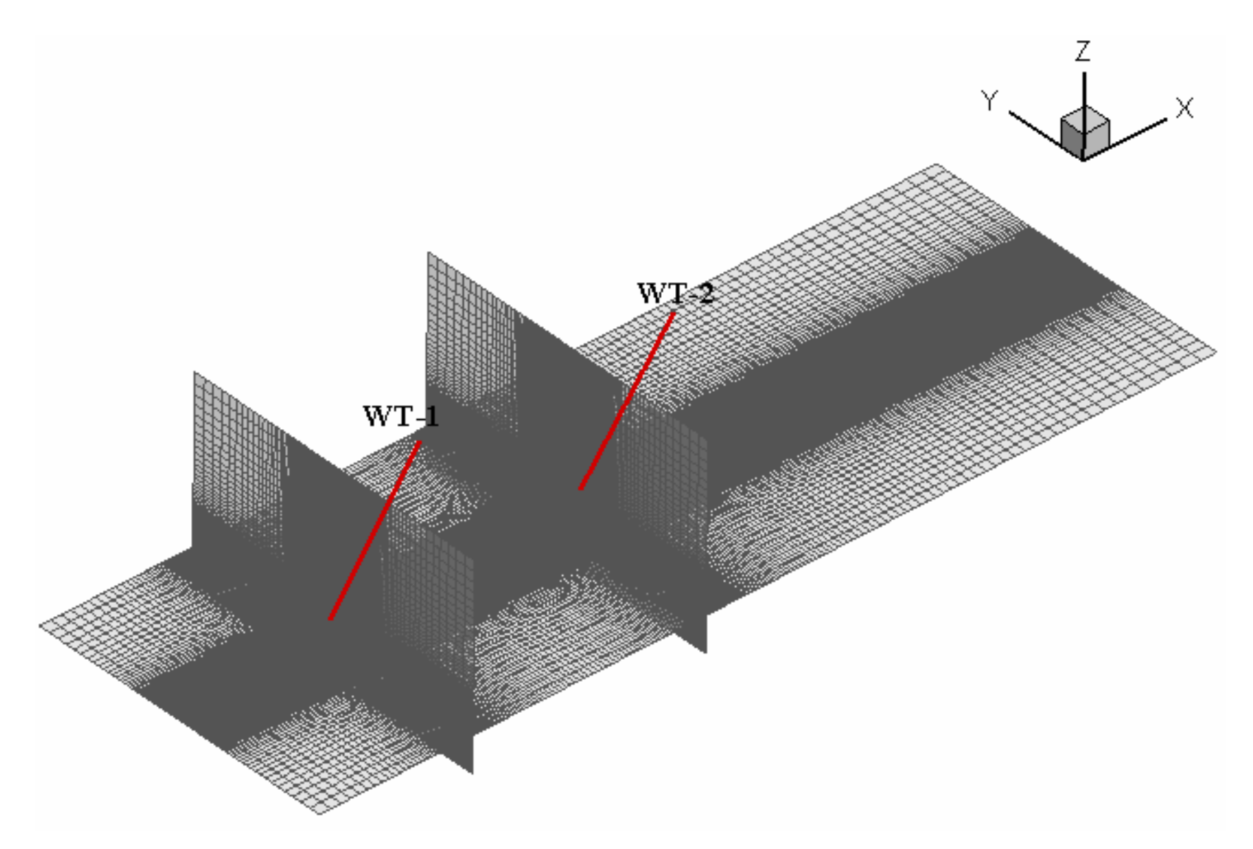
The G1 wind turbine’s physical domain is illustrated in Figure 2. The total length, width, and height of the calculated domain for the model verification were 15D × 3D × 3D, respectively. The wind turbine was placed in a dense area measuring 0.5D × 1.5D × 1.5D, the mesh size of the intensification area was 0.025 m, and the number of blade sections was 22. Structured grids were used in the computational domain. In the calculation, a constant inlet velocity of 5.0 m/s was given as the inlet boundary condition. The coordinate system was based on the origin of G1 and the upstream turbine (WT-1) shown in Figure 2a,b. In the figures, the inflow direction is represented by the x-axis, the horizontal radial direction is represented by the y-axis, and the vertical direction is represented by the z-axis. The staggered spacing between the upstream turbine (WT-1) and the downstream turbine (WT-2) in the y-axis direction is defined as staggered spacing (Δy).
As shown in Figure 2, the coordinate takes the center of the wind turbine hub as the origin, the x-axis is the wind turbine axial direction, the y-axis is the radial direction, and the z-axis is the vertical direction. The domain for NREL 5 MW wind turbines was 17D × 6D × 3D, and WT-1 and WT-2 were staggered with Δy: 0, 0.5R, 1.0R, 1.5R, and 2.0R. In all cases, the wind turbines were located in their respective near-field grid densification zones. The length, width, and height of the densification zone were 1D, 1.5D, and 1.5D, respectively. The wind turbine plane was located in the middle of the densification zone in the axial and longitudinal directions. Figure 3 shows a medium-density grid, WT-1 represents the upstream wind turbine, and WT-2 represents the downstream wind turbine. The mesh size of the densification zone was 3 m, and the mesh size outside the densification zone gradually transitioned to the densification zone, according to exponential law. The wind turbine blades, nacelles, and towers were all represented by volume force source terms, the number of blade sections was 18, and the number of tower sections was 25. All NREL 5 MW wind turbine configurations listed in the cases meshed with the same structured grid generation strategy. The reference wind speed at the hub height was 11.4 m/s [9].
The Grid Convergence Index (GCI) is recommended by the Fluids Engineering Division of the American Society of Mechanical Engineers as a reliable method for grid independence analysis [36]. The GCI was performed to evaluate the grid independence analysis results from the mesh resolution. GCI is defined as follows [37]:
G C I = δ r e 1
δ = φ f i n e φ m e d i u m φ f i n e
r = N f i n e N m e d i u m 1 / 3
e = 1 ln ( r ) ln φ m e d i u m φ c o a r s e φ f i n e φ m e d i u m
where φ is the simulated variable value of the simulation study for the k-th grid; N is the number of grids; δ is the relative error; r is the grid growth rate; e is the convergence order.
According to the model in Figure 2b, the number of grids for the simulation of NREL 5 MW wind turbines generated in this paper are 1.82 million (Coarse), 2.91 million (Medium), and 4.23 million (Fine). All the values of the above-defined quantities are listed in Table 3. The obtained results indicate that the medium mesh convergence has a GCI equal to 1.22%. Therefore, we have chosen 2.91 million (Medium) as the total number of grid cells in the calculation grid, which is used in the subsequent simulation to study the effects of staggered spacing on wind turbine characteristics.

2.3.3. Boundary Conditions and Model Settings

In this research, the CFD software Fluent 15.0 and the LES model were used for the simulation. The CFD solver was configured to be pressure-based, and the analysis was performed for an unsteady state. The UDF of the modified actuation line model in this paper was a program written in C language, which was then loaded into Fluent. The outlet of the flow field adopted the pressure outlet boundary condition, the top of the flow field adopted the symmetrical boundary condition, and the ground adopted the non-slip wall condition. The solution applied the pressure-velocity coupling of the COUPLED algorithm. The least-squares cell-based spatial discretization was used in the case of gradients, the pressure equation was discretized with second-order precision and second-order upwind in case of momentum, and energy and first-order upwind were used in case of turbulent dissipation rate. Meanwhile, the model convergence was defined based on the quantitative and qualitative monitoring of residuals [38].

3. Results and Discussion

3.1. Verification of the Modified Actuator Line Model

3.1.1. Analysis of Smoothing Parameters

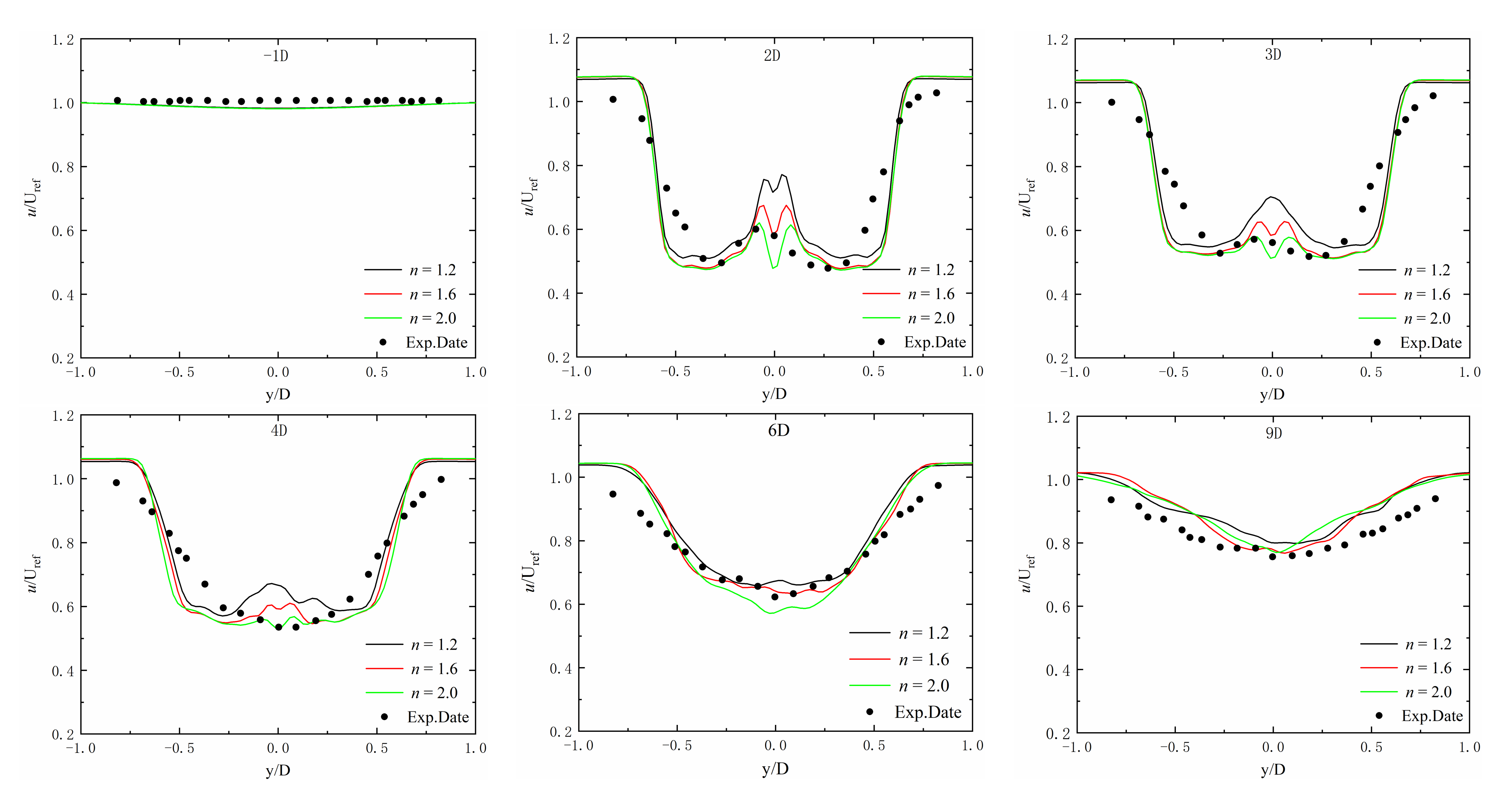
In the ALM, the volume force (Equation (10)) on the leaf element point is transferred to the surrounding grid cells through the three-dimensional Gaussian distribution method [39], and the value of the Gaussian distribution parameter ε is very important. The value of smoothing parameter ε is usually a multiple of the grid size in the wind plan rotation zone, that is, ε = n·DX, where n is Multiple and DX is the grid size of the rotation area. Figure 4 shows the Gaussian distribution function curves with different n. We chose n to be 1.2, 1.6, and 2.0 in three groups of cases, respectively, and then simulated the flow field of the G1 wind turbine under the condition of a 5.0 m/s uniform flow with MALM under the same condition of the densification zone’s grid size.
Table 4 shows the comparison between the thrust coefficient and power coefficient under different smoothing parameters. The axial thrust and output power of the wind turbine increase with the increase of ε. Among the three cases, the thrust coefficient and power coefficient calculated by n = 1.6 is the closest to the experimental values, while n = 1.2 underestimates the thrust and output power. It can be seen from Equation (10) that the force distribution around the blade becomes more uniform with the increase of ε, the influence area increases in size, and the volume force of the root and tip of the blade decreases, resulting in each leaf element on the blade being smaller. The axial inducing factor of the airfoil becomes smaller, the speed gradient changes smoothly, and the airfoil angle of attack increases, meaning that the load and output power of the blade become larger. As can be seen in Figure 5, in the far wake region (6D and beyond), the calculated velocity profiles are close to the experimental values, but in the near wake region (within 6D), the calculation results of n = 1.6 and n = 2.0 are relatively close. However, it should be noted that the case of n = 1.2 obtains a higher wake velocity near the root of the blade. The reason for this is that the range of the leaf element volume force at the leaf root decreases as ε decreases, meaning that the wind speed flowing through the area near the leaf root increases. The comprehensive comparison shows that when n = 1.6, the simulation accuracy of the MALM is more accurate. Therefore, n = 1.6 was selected in this research. With this in mind, the value of the Gaussian distribution parameter of the G1 wind turbine should be 1.6~2 times the mesh size of the dense zone (ε = 1.5~2.0DX). Jha [40] studied the NREL 5-MW turbine with the ALM and found that n provides the best prediction for all situations in the range of 1~3.4. Troldborg [22], meanwhile, suggested a Gaussian spreading width of n = 2.0 to maintain numerical stability. In this paper, the Gaussian distribution parameters in the actuation line simulation for the G1 wind turbine and NREL 5 MW turbine are both selected as 1.6.

3.1.2. Model Validation

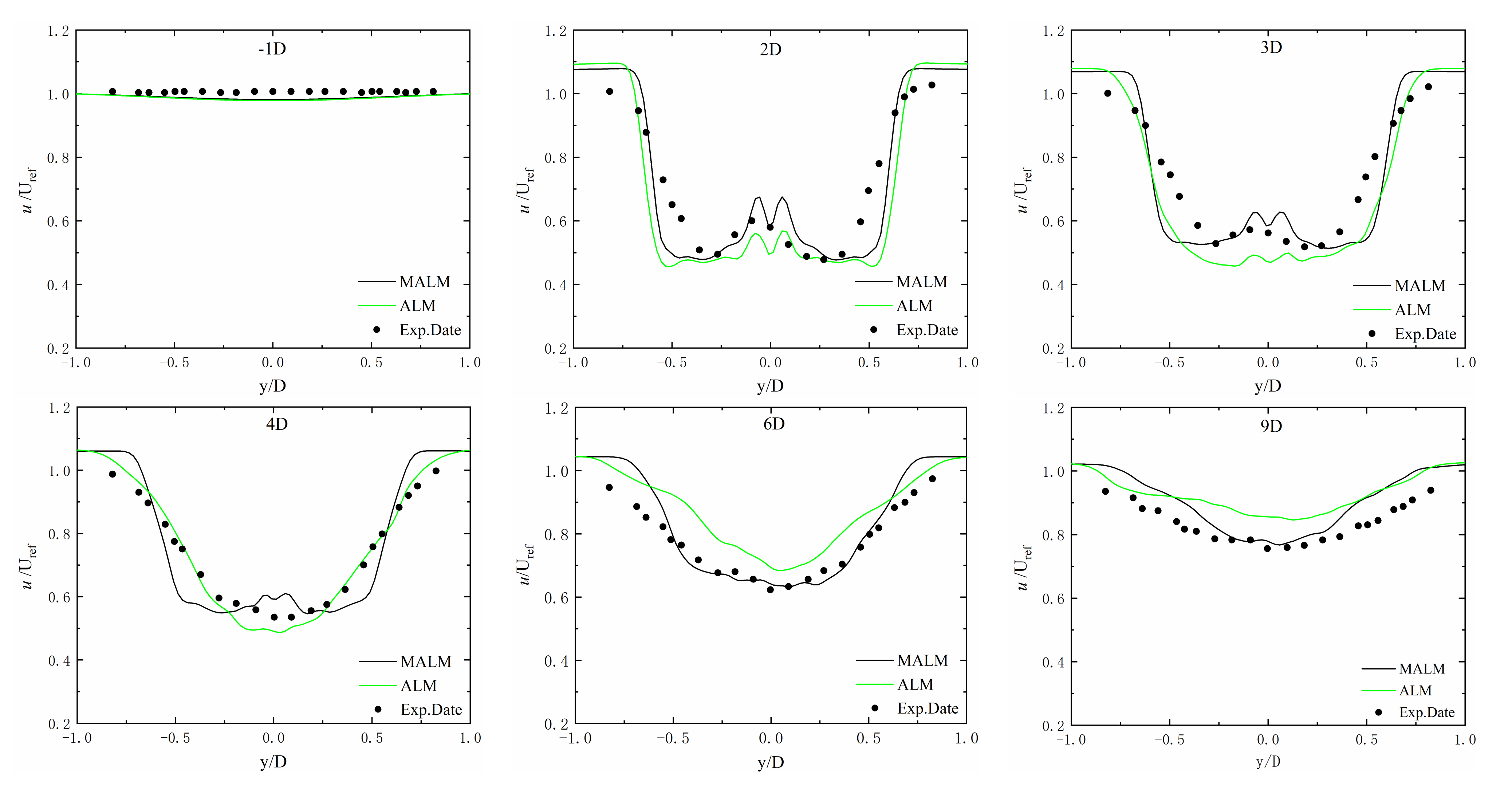
The simulation power and thrust coefficients of the G1 wind turbine are shown in Table 5. The MALM result is very close to the experimental value, and is better than the traditional ALM, particularly in the prediction of the thrust coefficient. This is because the MALM takes both the blade tip and root loss of the wind turbine into account.
Figure 6 shows the average wake velocity profiles in different locations at the hub height. Due to the revision on the tip and root loss, the center wake (y/D = 0) velocity of the MALM is closer to the experimental value than the traditional ALM. In the far wake, meanwhile, the MALM is more consistent with the experimental values. Traditional ALM attains a decent prediction accuracy of the thrust coefficient and power factor, but there are still some errors in the prediction of the center vortex and tip vortex due to blade tip and root losses. The MALM is suitable for calculating the flow field and aerodynamic characteristics of wind turbines.

3.2. Analysis of Staggered Spacing Conditions

3.2.1. Wind Turbine Output

Two NREL 5 MW wind turbines (WT-1 and WT-2) with different staggered spacing (Δy) were simulated to study the effect of the staggered spacing on the characteristics of wind turbines. From Figure 7, we can see that both the output power and thrust of the WT-1 gradually decrease before stabilizing after 7 weeks of rotation (the rated speed of the rotor is 12.1 rpm, so the rotor rotates will be 7 times at t = 35 s). The standard deviation first increases and then decreases as the staggered spacing Δy increases. Meanwhile, when under the same case, the standard deviation of power and the thrust of WT-1 are smaller than those of WT-2, which indicates that WT-2 fluctuates greatly. The stabilized power and thrust values were approximately 5.9 MW and 743 KN, respectively. When the WT-1 wake reaches the WT-2 plane, the WT-2 output power and thrust have a period of large fluctuations due to wake disturbance, before gradually stabilizing. Compared with the conditions Δy = 0.5R and Δy = 2R, the results of Δy = 1.0R and Δy = 1.5R fluctuated highly, especially Δy = 1.0R. The fluctuation power range was approximately between 2.25 MW and 4.50 MW, and the thrust was between 450 KN and 600 KN, approximately. For Δy = 0.5R, which is influenced by the expansion of the WT-1 wake, the WT-2 wind turbine plane is mostly in the wake of WT-1, so the three blades are subjected to smaller differences in velocity and weaker fluctuations in the rotation cycle. For the Δy = 2R condition, the aerodynamic power generation characteristics of WT-2 are less influenced by the wake disturbance of the upstream WT-1. When the flow is fully developed and stable, the output power and thrust of the four cases are, in order, 2.25 MW, 3.40 MW, 5.20 MW, 5.75 MW, and 450 KN, 535 KN, 725 KN, and 77 5 KN.
As can be seen in Figure 8, with the increase in staggered spacing Δy, both the power and thrust fluctuations in a rotation cycle initially increase and then decrease. In addition, the fluctuation amplitude becomes higher, meaning that the blades experience significant turbulence during rotation. As WT-2 is a three-blade structure, both the output power and the thrust decrease significantly when one blade is passing through the wake center of WT-1, which seems to be caused by the center vortex of the wake. This phenomenon is observed three times every rotor turn at the azimuth angles of 60+, 180+, and 270+. In the case of Δy = 0.5R, the WT-2 power decreases by 33.3% and the thrust decreases by 11.2% compared with the average results when one blade passes through the wake center of WT-1. In comparison with Δy = 0.5R, the maximum loss of power and thrust in the case of Δy = 1.5R is reduced by half. The output power and thrust fluctuate most widely under the Δy = 1.5R condition. Contrastingly, Δy = 2R only causes small dips in power. Furthermore, the peaks widen, resulting in the rotor being exposed in the long term to the unsteady wake of WT-1, and the output power is also unstable.
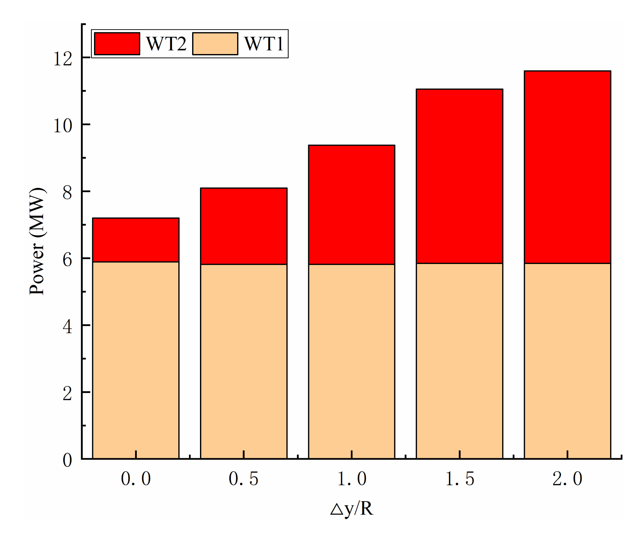
Figure 9 shows the power capture of WT-1 and WT-2 for each case. When the staggered spacing Δy increases, the power capture of WT-1 becomes stable, while the output power of WT-2 increases with the total power. The WT-2 output power shows a trend of initially rapidly increasing then slowing down. When the staggered spacing is Δy = R and 1.5R, the WT-2 inflow velocity is unevenly distributed, one part of WT-2′s plane is still in the low-speed wake of WT-1, the other part is in free-flow, and the WT-2 power capture increases as the staggered spacing increases. When the staggered spacing between the two wind turbines continues to increase, the amount of WT-2 located in the wake of WT-1 decreases, and the mutual interference between the two wind turbines gradually weakens, which causes the output power to stabilize. When the staggered spacing is Δy = 2R, the output power of WT-2 is less affected by WT-1.

3.2.2. Analysis of Coupling Fields

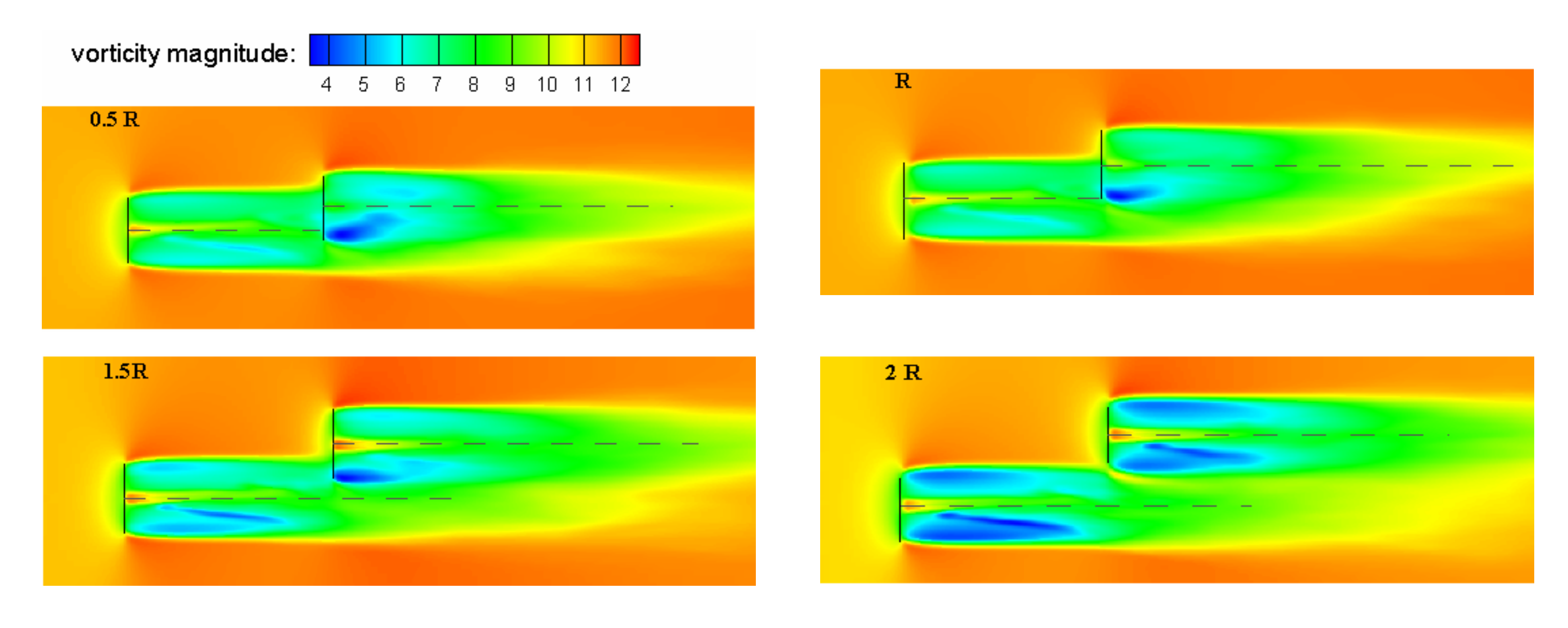
As shown in Figure 10, with the increase of staggered distance Δy, the wake centerline of WT-1 gradually deviates from the wind turbine’s plane of WT-2, and the wake interaction between WT-1 and WT-2 is gradually weakened. A low wind speed zone is prone to appear beneath the wake centerline of WT-2. Then, as the airflows mix, the low-speed area gradually expands in the tangential direction of the entire wake until making it slowly recover. The incoming WT-1 flow is free-flow, and the wake is distributed symmetrically along the centerline. Whilst part of the WT-2 rotor plane is in the wake of WT-1 and the other part is in free-flow, the wake is asymmetrically distributed along the centerline. The significant difference in air velocity and turbulence intensity causes an uneven force on the blades, leading to periodic fluctuations in power capture, and increasing fatigue load on the turbine that can prematurely wear down the turbine hardware.
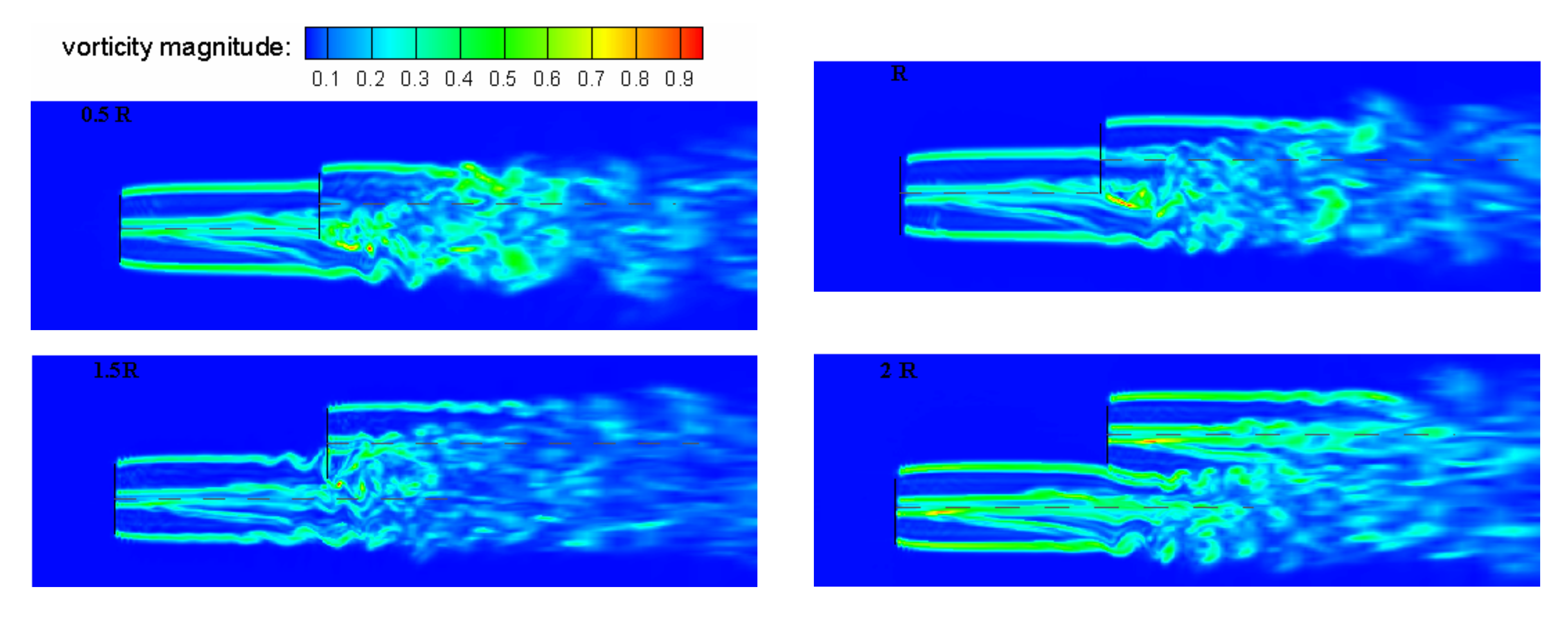
As shown in Figure 11, since the incoming flow of WT-1 is undisturbed and the tip speed ratio is stable, a clearer tip vortex and root vortex are generated in the wake. As the wake flows downstream, the WT-1 wake vortex gradually breaks or fuses into WT-2’s wake vortex, causing it to become more chaotic. In addition, the wake interaction effect is strong. In the case of Δy = 0.5R, since most of the wind rotor plane is located in the wake of WT-1, it is difficult to see the tip vortex and root vortex produced by WT-2. The structure of the vortex system in the superimposed wake is also chaotic, which results in the fast recovery of the wake (Figure 12). In the other three cases, at least half of the WT-2 wind turbine plane is not in the wake of WT-1, so the tip vortex of WT-2 can be observed clearly. When Δy = 2R, the phenomenon whereby wind turbine tail vortex structures in the upstream and downstream affect each other almost disappears, and the vortices generated by the two wind turbines develop freely and move downstream until they enter the rupture stage.
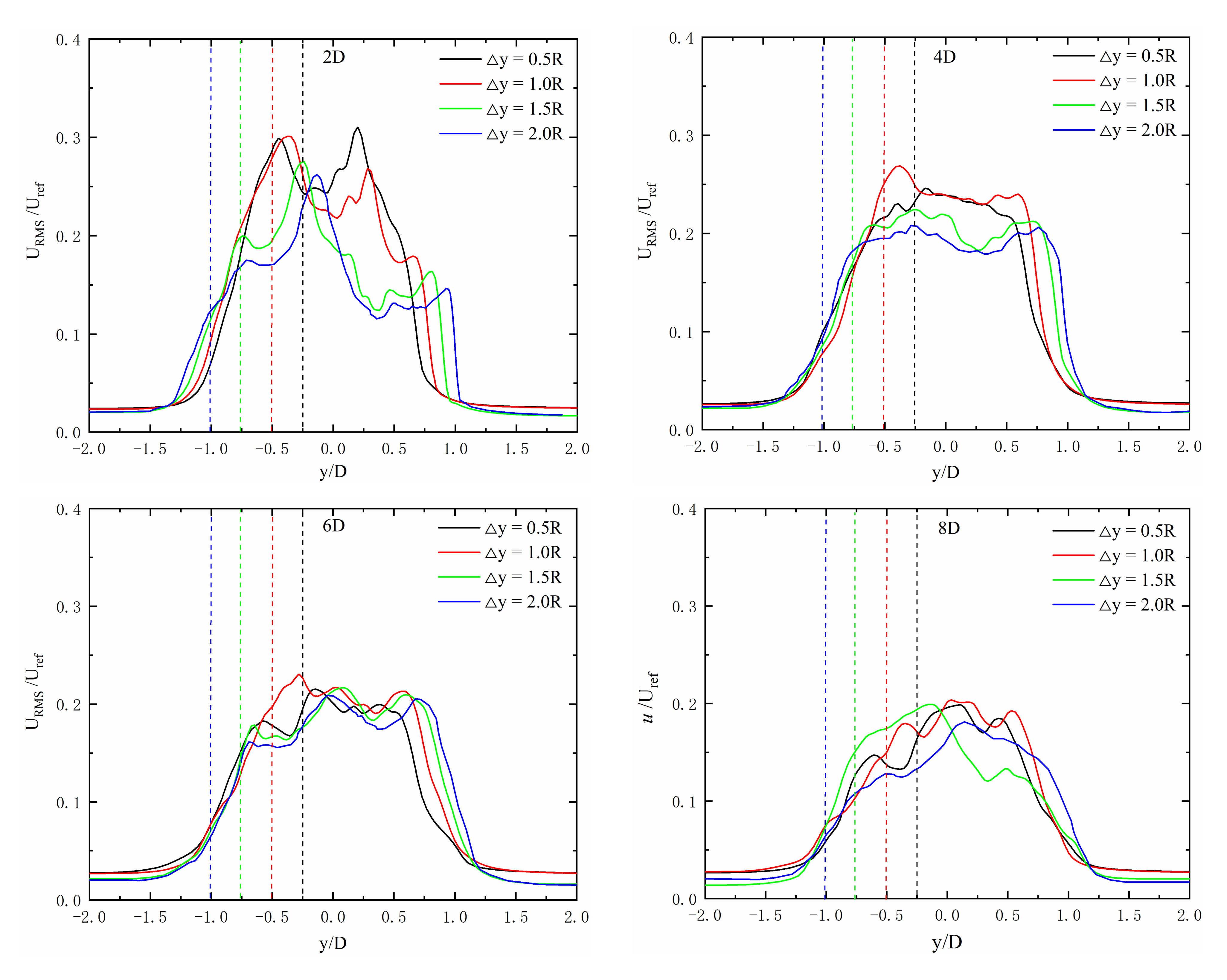
Figure 12 shows the normalized velocity profiles behind WT-2 at different axial locations at the hub height. As the distance Δy increases, the WT-2 wake in the -y-axis range is affected by the wake of WT-1. Therefore, the axial width of the WT-2 wake increases, and the wake becomes more complex. The velocity distribution in the wake overlap area (-y-axis range) of WT-2 and WT-1 is quite different, but the +y axis range is farther away from the WT-1 wake centerline, so the difference of velocity distribution is small. When the velocity in the near-wake (2D, 4D) of WT-2 is added to the increase of Δy in the wake center, the difference of velocity in the near-wake becomes larger. As the wake develops downstream, the difference in wake distribution between the different cases decreases, and the recovery of the wake is obvious after 8D. The center velocity of the far wake region (6D, 8D) of WT-2 recovers slowly while the velocity in the y < −1.0D region recovers faster, indicating that the wake recovery of WT-2 slows down with an increase in Δy. As shown in Figure 13, the turbulence is decreased as the distance Δy increases; meanwhile, the radial range (y-axis) of the turbulent mixing zone becomes wider.

4. Conclusions

This study modified the full-scale actuator line model, including blades, nacelles, and towers, and combined it with the LES method to verify the model against the G1 turbine. The wake characteristics of two NREL 5MW wind turbines (WT-1 and WT-2) with different staggered arrangements Δy were individually simulated to explore the influence of the upstream wind turbine wake and the working state on the downstream wind turbine output power and wake vortex structure. The conclusions drawn are as follows:
(1)
The MALM is verified by the G1 experimental turbine with a uniform wind speed of 5.0 m/s. The thrust coefficient, power coefficient, and wake velocity of the wind turbine were all consistent with the experimental values. Under the condition of the smoothing parameter ε = 1.6DX, the simulated values of the thrust and power of MALM are more accurate, and the wake distribution is also close to the experimental values.
(2)
In the case of Δy = R, and 1.5R, the output power and thrust of WT-2 decreased significantly when one of three blades was passing near the center vortex of WT-1. This phenomenon was observed three times per rotor revolution at the azimuth angles of 60+, 180+, and 270+. In the case of Δy = 0.5R, the power of WT-2 decreased by 33.3%, and the thrust decreased by 11.2% compared with the average results of when only one blade passed near the wake center of WT-1. In comparison with Δy = 0.5R, the maximum loss of power and thrust was reduced by half, to Δy = 1.5R. Furthermore, the peaks are significantly wider than Δy = 0.5R, resulting in longer periods of an unstable fatigue load on the blade, and unstable output power. Contrastingly, Δy = 2R and 0.5R only cause small dips in power.
(3)
As the staggered spacing Δy increased, the output power of WT-1 stabilized at 5.9 MW, and the total output power was enhanced. When the staggered spacing between the two wind turbines continued to increase, the part of the WT-2 plane located in the wake of WT-1 decreased, and the wake was asymmetrically distributed along the centerline. The significant difference in air velocity and turbulence intensity causes an uneven force on the wind turbine blades, and the mutual interference between the two wind turbines gradually weakens. Following this, the output power then slows down and stabilizes.
(4)
With an increase in staggered spacing Δy, the axial extent of the wake width increases, the wake becomes more complex, and the velocity of WT-2 is added to the wake center, making the difference of velocity in the near-wake larger. It is observed that the wake of WT-2 recovery slows down with the increase of Δy. Along with the main wind, the output power of WT-2 will fluctuate greatly, and the wake will become complex with 0.5R < Δy < 1.5R, which is not conducive to a safe and stable operation of downstream wind turbines.

Author Contributions

Writing and investigation, F.X.; data curation and software, H.D.; methodology and funding acquisition, C.X.; writing and investion, X.H.; funding acquisition and editing, Y.S.; writing, T.L.; writing, Z.F. All authors have read and agreed to the published version of the manuscript.

Funding

This research was funded by the Research on smart operation control technologies for offshore wind farms (Grant No. 2019YFE0104800), National Science Foundation of China-Yalong River Joint Fund (Grant No. U1865101), Fundamental Research Funds for the Central Universities (Grant No. B200203057), Postgraduate Research & Practice Innovation Program of Jiangsu Province (Grant No. KYCX20_0470), the Jiangsu Province Science Foundation for Youths (Grant No. BK20180505), Basic research program of Jiangsu Province (Grant No. BK20200182), the fellowship of China Postdoctoral Science Foundation (Grant No. 2020M671314), Open Fund of Key Laboratory of Icing and Anti/De-icing (Grant No. IADL20190302), and the Priority Academic Program Development of Jiangsu Higher Education Institutions.

Institutional Review Board Statement

This paper does not involve humans or animals.

Informed Consent Statement

The study in this paper did not involve humans.

Data Availability Statement

The data that support this manuscript are available from Chang Xu upon reasonable request.

Acknowledgments

Authors would like to acknowledgment Li Linmin from Zhejiang Sci-Tech University for theoretical support.

Conflicts of Interest

We have read the agreement, agreed to publish this paper, and declare no conflict of interest.

Abbreviations

ALMActuator line model
MALMModified actuator line model
BEMBlade element theory
LESLarge eddy simulation
WT-1Upstream wind turbine
WT-2Downstream wind turbine
ΔyStaggered spacing of two wind turbines in the y-axis direction
NRELNational Renewable Energy Laboratory
CFDComputational Fluid Dynamics
N-SNavier–Stokes
UDFUser-Defined Function
PANSPartially-Averaged Navier–Stokes
GCIThe grid convergence index

Nomenclature

x, y, zCoordinates
xwt, ywt, zwtThree-dimensional coordinates of the hub center of the wind turbine
ρAir density, kg/m3
u Three-dimensional velocity vector
pPressure acting on the fluid micro-element, Pa
fiVolume force, KN
μDynamic viscosity, N·s/m2
uiAveraged velocity in the i-th direction, m/s
ΦRotation angle of the blade i in the current time step, deg
ΥStarting phase angle of the blade, deg
BNumber of blades
δRotation angle of the blade in the current time step, deg
ωRotational angular velocity of the turbine rotor, rad/s
tTime of rotation, s
xiCoordinate of the blade element point, m
xi_cellGrid cell centroid coordinate, m
DXiGrid cell size, m
uiVelocity at the blade element point, m/s
ucellGrid centroid velocity closest to the blade element point, m/s
u Velocity gradient of the flow field
dSDistance from the blade element point to the nearest grid centroid
cChord length of the airfoil, m
ClLift coefficient
CdDrag coefficient
φInflow angle, deg
βTwist angle, deg
drBlade element span
dDistance between M and blade element, m
εSmoothing parameter
RRadius of the blade, m
DDiameter of the turbine rotor, m
RhubRadius at the root of the rotor of the turbine, m
αmaxAngle of attack according to the maximum lift coefficient
α0Angle of attack according to the zero-lift coefficient
nEmpirical value, 1.0
dfx,towAirflow axial resistance of a tower element
UWind speed, m/s
FnacNacelle resistance
utowIncoming wind speed at the center of the tower element, m/s
dtowCircular cross-sectional diameter of the center of the tower element, m
dhElement height of the tower, m
CD,towResistance coefficient of the tower, 1.0
AnacCross-sectional area of the nacelle, m2
CD,nacResistance coefficient of the nacelle, 1.0
zHeight above the ground, m
κVon Karman constant, 0.4187
u*Friction velocity, m/s
z0Surface roughness, m
nMultiple
DXthe grid size, m
φthe simulated variable value of the simulation study for the k-th grid
fεthe volume force after smoothing
fthe volume force on the blade element
Bthe number of blades
fijthe volume force on a leaf element point
δthe relative error
rthe grid growth rate
ethe convergence order
Urefthe reference wind speed, m/s
URMSthe root mean square of wind speed

References

  1. Kim, H.-G.; Kim, J.-Y. Analysis of wind turbine aging through operation data calibrated by LiDAR measurement. Energies 2021, 14, 2319. [Google Scholar] [CrossRef]
  2. Howland, M.F.; Dabiri, J.O. Influence of wake model superposition and secondary steering on model-based wake steering control with SCADA data assimilation. Energies 2021, 14, 52. [Google Scholar] [CrossRef]
  3. Martinez-Tossas, L.A.; Churchfield, M.J.; Leonardi, S. Large eddy simulations of the flow past wind turbines: Actuator line and disk modeling. Wind Energy 2015, 18, 1047–1060. [Google Scholar] [CrossRef]
  4. Kim, T.; Oh, S.; Yee, K. Improved actuator surface method for wind turbine application. Renew. Energy 2015, 76, 16–26. [Google Scholar] [CrossRef]
  5. Ivanell, S.; Sørensen, J.N.; Mikkelsen, R.; Henningson, D. Analysis of numerically generated wake structures. Wind Energy 2009, 12, 63–80. [Google Scholar] [CrossRef]
  6. Ivanell, S.; Mikkelsen, R.; Sørensen, J.N.; Henningson, D. Stability analysis of the tip vortices of a wind turbine. Wind Energy 2010, 13, 705–715. [Google Scholar] [CrossRef]
  7. Shen, W.Z.; Zhu, W.J.; Sorensen, J.N. Actuator line/Navier-Stokes computations for the MEXICO rotor: Comparison with detailed measurements. Wind Energy 2012, 15, 811–825. [Google Scholar] [CrossRef]
  8. Fredriksson, S.T.; Broström, G.; Bergqvist, B.; Lennblad, J.; Nilsson, H. Modelling Deep Green tidal power plant using large eddy simulations and the actuator line method. Renew. Energy 2021, 179, 1140–1155. [Google Scholar] [CrossRef]
  9. Qian, Y.; Wang, T.; Yuan, Y.; Zhang, Y. Comparative study on wind turbine wakes using a modified partially-averaged navier-stokes method and large eddy simulation. Energy 2020, 206, 118147. [Google Scholar] [CrossRef]
  10. Baratchi, F.; Jeans, T.L.; Gerber, A.G. A modified implementation of actuator line method for simulating ducted tidal turbines. Ocean Eng. 2019, 193, 106586. [Google Scholar] [CrossRef]
  11. Réthoré, P.; van der Laan, P.; Troldborg, N.; Zahle, F.; Sørensen, N.N. Verification and validation of an actuator disc model. Wind Energy 2014, 17, 919–937. [Google Scholar] [CrossRef]
  12. Martínez-Tossas, L.A.; Meneveau, C.; National Renewable Energy Lab (NREL). Filtered lifting line theory and application to the actuator line model. J. Fluid Mech. 2019, 863, 269–292. [Google Scholar] [CrossRef]
  13. Tabib, M.; Rasheed, A.; Kvamsdal, T. Investigation of the impact of wakes and stratification on the performance of an onshore wind farm. Energy Procedia 2015, 80, 302–311. [Google Scholar] [CrossRef] [Green Version]
  14. Xie, S.; Archer, C.L.; Ghaisas, N.; Meneveau, C. Benefits of collocating vertical-axis and horizontal-axis wind turbines in large wind farms. Wind Energy 2017, 20, 45–62. [Google Scholar] [CrossRef]
  15. Zhang, M.; Arendshorst, M.G.; Stevens, R.J.A.M. Large eddy simulations of the effect of vertical staggering in large wind farms. Wind Energy 2019, 22, 189–204. [Google Scholar] [CrossRef]
  16. Meyers, J.; Meneveau, C. Optimal turbine spacing in fully developed wind farm boundary layers. Wind Energy 2012, 15, 305–317. [Google Scholar] [CrossRef] [Green Version]
  17. Albatal, S.A.; Mohamed, M.H. Optimization of H-Rotor Darrieus turbines’ mutual interaction in staggered arrangements. Renew. Energy 2018, 125, 87–99. [Google Scholar] [CrossRef]
  18. Parada, L.; Herrera, C.; Flores, P.; Parada, V. Assessing the energy benefit of using a wind turbine micro-siting model. Renew. Energy 2018, 118, 591–601. [Google Scholar] [CrossRef]
  19. Hezaveh, S.H.; Bou-Zeid, E.; Dabiri, J.; Kinzel, M.; Cortina, G.; Martinelli, L. Increasing the power production of vertical-axis wind-turbine farms using synergistic clustering. Bound. Layer Meteorol. 2018, 169, 275–296. [Google Scholar] [CrossRef] [Green Version]
  20. Nilsson, K.; Shen, W.Z.; Sørensen, J.N.; Breton, S.-P.; Ivanell, S. Validation of the actuator line method using near wake measurements of the MEXICO rotor. Wind Energy 2015, 18, 499–514. [Google Scholar] [CrossRef]
  21. Gao, Z.; Li, Y.; Wang, T.; Ke, S.; Li, D. Recent improvements of actuator line-large-eddy simulation method for wind turbine wakes. Appl. Math. Mech. 2021, 42, 511–526. [Google Scholar] [CrossRef]
  22. Troldborg, N.; Sorensen, J.N.; Mikkelsen, R. Actuator line simulation of wake of wind turbine operating in turbulent inflow. In Journal of Physics: Conference Series; IOP Publishing: Bristol, UK, 2007. [Google Scholar] [CrossRef]
  23. Martinez-Tossas, L.A.; Churchfield, M.J.; Yilmaz, A.E.; Sarlak, H.; Johnson, P.L.; Sorensen, J.N.; Meyers, J.; Meneveau, C. Comparison of four large-eddy simulation research codes and effects of model coefficient and inflow turbulence in actuator-line-based wind turbine modeling. J. Renew. Sustain. Energy 2018, 10, 33301. [Google Scholar] [CrossRef] [Green Version]
  24. Campagnolo, F.; Petrovi, V.; Schreiber, J.; Nanos, E.M.; Croce, A.; Bottasso, C.L. Wind tunnel testing of a closed-loop wake deflection controller for wind farm power maximization. In Journal of Physics: Conference Series; IOP Publishing: Bristol, UK, 2016; Volume 753. [Google Scholar] [CrossRef] [Green Version]
  25. Campobasso, M.S.; Baba-Ahmadi, M.H. Analysis of unsteady flows past horizontal axis wind turbine airfoils based on harmonic balance compressible Navier-Stokes equations with low-speed preconditioning. J. Turbomach. 2012, 134, 61020. [Google Scholar] [CrossRef] [Green Version]
  26. Felten, F.; Fautrelle, Y.; Du Terrail, Y.; Metais, O. Numerical modeling of electromagnetically-riven turbulent flows using LES methods. Appl. Math. Model. 2004, 28, 15–27. [Google Scholar] [CrossRef] [Green Version]
  27. Shen, W.Z.; Mikkelsen, R.; Sørensen, J.N.; Bak, C. Tip loss corrections for wind turbine computations. Wind Energy 2005, 8, 457–475. [Google Scholar] [CrossRef]
  28. Corrigan, J.J.; Schilling, J.J. Empirical model for stall delay due to rotation. In Proceedings of the American Helicopter Society Aeromechanics Specialists Conference, San Francisco, CA, USA, 19–21 January 1994. [Google Scholar]
  29. Shives, M.; Crawford, C. Mesh and load distribution requirements for actuator line CFD simulations: Mesh and load distribution requirements for actuator line simulations. Wind Energy 2012, 16, 1183–1196. [Google Scholar] [CrossRef]
  30. Santoni, C.; Carrasquillo, K.; Arenas-Navarro, I.; Leonardi, S. Effect of tower and nacelle on the flow past a wind turbine. Wind Energy 2017, 20, 1927–1939. [Google Scholar] [CrossRef]
  31. Richards, R. Appropriate boundary conditions for computational wind engineering models using the k-ϵ turbulence model. J. Wind Eng. Ind. Aerodyn. 1993, 46, 145–153. [Google Scholar] [CrossRef]
  32. Takizawa, K.; Henicke, B.; Tezduyar, T.E.; Hsu, M.; Bazilevs, Y. Stabilized space–time computation of wind-turbine rotor aerodynamics. Comput. Mech. 2011, 48, 333–344. [Google Scholar] [CrossRef]
  33. Draper, M.; Guggeri, A.; Mendina, M.; Usera, G.; Campagnolo, F. A large eddy simulation-actuator line model framework to simulate a scaled wind energy facility and its application. J. Wind Eng. Ind. Aerodyn. 2018, 182, 146–159. [Google Scholar] [CrossRef]
  34. Nejad, A.R.; Guo, Y.; Gao, Z.; Moan, T.; National Renewable Energy Lab (NREL). Development of a 5 MW reference gearbox for offshore wind turbines: 5 MW reference gearbox. Wind Energy 2015, 19, 1089–1106. [Google Scholar] [CrossRef] [Green Version]
  35. Yu, Z.; Zheng, X.; Ma, Q. Study on actuator line modeling of two NREL 5-MW wind turbine wakes. Appl. Sci. 2018, 8, 434. [Google Scholar] [CrossRef] [Green Version]
  36. Sosnowski, M. Evaluation of heat transfer performance of a multi-disc sorption bed dedicated for adsorption cooling technology. Energies 2019, 12, 4660. [Google Scholar] [CrossRef] [Green Version]
  37. Roache, P. Perspective—A method for uniform reporting of grid refinement studies. J. Fluids Eng. 1994, 116, 405–413. [Google Scholar] [CrossRef]
  38. Zhang, W.; Wang, Y.; Shen, Y.; Wang, Y.; Xu, Y.; Zhang, X. CFD studies of wake characteristics and power capture of wind turbines with trailing edge flaps. IEEE Access 2020, 8, 7349–7361. [Google Scholar] [CrossRef]
  39. Martínez-Tossas, L.A.; Churchfield, M.J.; Meneveau, C. Optimal smoothing length scale for actuator line models of wind turbine blades based on gaussian body force distribution. Wind Energy 2017, 20, 1083–1096. [Google Scholar] [CrossRef]
  40. Jha, P.K.; Churchfield, M.J.; Moriarty, P.J.; Schmitz, S. Guidelines for volume force distributions within actuator line modeling of wind turbines on large-eddy simulation-type grids. J. Sol. Energy Eng. 2014, 136, 31003. [Google Scholar] [CrossRef]
Figure 1. Actuator line model. (a) Rotation of the wind rotor; (b) Triangle of the blade element.
Energies 15 00282 g001
Figure 2. The physical domain used in this study: (a) Wind turbine G1; (b) NREL 5 MW wind turbines with a staggered arrangement.
Energies 15 00282 g002
Figure 3. Medium-density mesh in the computational domain.
Energies 15 00282 g003
Figure 4. Gaussian distribution function curves with different n.
Energies 15 00282 g004
Figure 5. Average radial distribution velocity profiles in different locations under different smoothing parameters. The black points represent the experimental data [33] (Uref = 5 m/s). Reprint with permission 5219051009765; Copyright 2018, Elsevier.
Energies 15 00282 g005
Figure 6. Average wake velocity profiles in different locations at the hub height. The black points represent the experimental data [33] (Uref = 5 m/s). Reprint with permission 5219051009765; Copyright 2018, Elsevier.
Energies 15 00282 g006
Figure 7. Aerodynamic output power and turbine thrust during simulation time. (a) Output power of WT-1 (the standard deviations are 0.08, 0.08, 0.12, and 0.08, respectively); (b) Thrust of WT-1 (the standard deviations are 4.37, 4.29, 12.82, and 4.15, respectively); (c) Output power of WT-2 (the standard deviations are 0.29, 0.66, 0.45, and 0.08, respectively); (d) Thrust of WT-2 (the standard deviations are 31.74, 46.85, 28.13, and 5.29, respectively).
Energies 15 00282 g007
Figure 8. Profiles of the aerodynamic power and turbine thrust of WT-2 during the last calculated rotation (with blade 1 vertically upward). (a) The output of power; (b) Thrust.
Energies 15 00282 g008
Figure 9. The output power of WT-1 and WT-2 for each case.
Energies 15 00282 g009
Figure 10. Mean streamwise velocity component of the horizontal section of the wind turbine center. The model turbine rotor is the sketched black line, and the dotted line represents the wake flow center.
Energies 15 00282 g010
Figure 11. Vorticity contour of the horizontal section of the wind turbine center. The model wind turbine is sketched in black, and the dotted line represents the wake flow center.
Energies 15 00282 g011
Figure 12. Normalized velocity profiles behind WT-2 at different axial locations in the hub height. The dotted line represents the wake centerline of the WT-1 under each Δy (Uref = 11.4 m/s).
Energies 15 00282 g012
Figure 13. Turbulence behind WT-2 at different axial locations in the hub height. The dotted line represents the wake centerline of the WT-1 under each Δy (Uref = 11.4 m/s).
Energies 15 00282 g013
Table 1. Parameters of the wind turbine G1.
DiameterBlade RadiusHub DiameterTower HeightRated VelocityAirfoil
1.1 m0.55 m0.03 m0.8 m850 rpmRG14
Table 2. Overview of the NREL 5 MW reference turbine.
DiameterBlade RadiusRated SpeedTower HeightRated VelocityRated Power
126 m61.5 m11.4 m/s90 m12.1 rpm5.3 MW
Table 3. Grid independence study.
ParameterCoarseMediumFine
φ/KN726743751
N/1061.822.914.23
δ-0.020.01
r-1.171.13
e-6.17-
GCI/%-1.220.89
Table 4. Comparison of thrust and power coefficients of a wind turbine under different smoothing parameters.
Parametern = 1.2n = 1.6n = 2.0
CtCpCtCpCtCp
Experimental value0.7880.4530.7880.4530.7880.453
Simulated results0.7490.4070.7910.4570.8010.470
Difference (%)−4.90−10.250.380.881.633.71
Table 5. Power and thrust coefficients of the G1 wind turbine.
ModelMALMALM
ParameterCtCpCtCp
Experimental value0.7880.4530.7880.453
Simulated results0.7910.4570.9610.472
Difference (%)0.380.8821.954.19
Publisher’s Note: MDPI stays neutral with regard to jurisdictional claims in published maps and institutional affiliations.