Development of New Protection Scheme in DC Microgrid Using Wavelet Transform

Abstract

The demand for a low voltage direct current (LVDC) microgrid is increasing by the increase of DC-based digital loads and renewable resources and the rapid development of power electronics technology. For the stable operation of an LVDC microgrid, it is necessary to develop a protection method. In this paper, the new protection scheme considering the fault section is proposed using wavelet transform (WT) in an LVDC microgrid. The fault sections are classified into DC side of the alternating current (AC)/DC converter, DC/DC converter connected to photovoltaic (PV) system, DC line, and DC bus. The characteristics of fault current at each fault section are analyzed. Based on these analyses, the new protection scheme including the fault section estimation is proposed using WT. The proposed scheme estimates the fault section using the detail component after performing WT and sends the trip signal to each circuit breaker according to the fault section. The proposed protection scheme is verified through various simulations according to the fault region and fault current using electromagnetic transient program (EMTP)/ATPDraw and MATLAB. The simulation results show that the fault section is accurately determined, and the corresponding circuit breaker (CB) operations are performed.

1. Introduction

The demand for the development of a low voltage direct current (LVDC) distribution technology is increasing with expectations for the rapid development of power conversion technology, the increase in direct current (DC)-based digital loads, and the expansion of DC-based renewable energy, energy storage devices, and electric vehicles. The DC power supply method reduces power losses through high-efficiency conversion, which reduces the number of alternating current (AC)/DC power conversions, and it can be an effective countermeasure to help combat global warming. Therefore, it is necessary to improve energy efficiency and power quality and to increase system reliability by developing technology for steady-state operation and protection technology for transient states in the LVDC distribution network. In this study, we have focused on the protection technology to judge electrical faults, to isolate the fault sections, and to maintain the normal power supply to non-faulted sections. If the fault is not detected and isolated from the system quickly, the disturbance may be applied to the converter composed of a solid state switch. Therefore, the life reduction of converter and the reliability degradation such as mean time between failure (MTBF) on the power system are expected [1,2,3,4,5]. Therefore, it is important to develop a protection scheme for fast fault detection and isolation.

Various studies of protection have been conducted on LVDC distribution systems. In [6], a method for fast DC fault detection and interruption was proposed using advanced local measurements and communications available in a smart grid. In [7], a method to detect and locate DC faults was proposed using several intelligent relays based on the DC current direction and combined with controllable solid-state circuit breakers. In [8], a method using the first and second derivatives of the fault current was proposed to classify faulty and non-faulty situations. In [9], the transient response of a hybrid AC/DC LV distribution system was analyzed, and a protection method for each system was proposed. In [10], the use of fuses for short-circuit protection in LVDC systems was evaluated. In [11], a hybrid passive-overcurrent relay consisting of an inductor, a capacitor, and one current and one voltage transducer was proposed. In that study, the relay used a conventional overcurrent function for low-resistance fault detection, and a real-time discrete wavelet transform was used for high-resistance fault detection. In [12], a fault detection method based on an equivalent inductance estimation that does not require communication equipment was proposed. In [13], a mathematical morphology-based protection method was proposed using the features from fault currents with capacitor discharge characteristics or high-impedance faults with arcing phenomenon. In [14], a fault detection method was proposed using the advantages of overcurrent, primary and secondary differentiation of current, and signal processing techniques. In [15], a protection method in a ring-bus LVDC microgrid with intelligent electronic equipment and a solid-state circuit breaker was proposed. In [16], low-resistance and high-resistance faults were distinguished, and a fault detection and location estimation method using the voltage applied to the inductor for low-resistance faults and the ground fault current for high-resistance faults was proposed. In [17], a fault-area detection method was proposed using the capacitor discharge current. In [18], a new protection method was proposed combining the change in voltage (dv/dt) and the change in current (di/dt). These previous studies have suggested fault detection methods, but have not proposed an adaptive protection method in connection with the fault section determination. Therefore, in this study, a protection method is proposed considering the fault section. In addition, the existence of a photovoltaic (PV) power generation system, which has not been considered before, is also considered.

Wavelet transform (WT) is a mathematical method that is widely used in various fields, such as signal and image processing. The WT can be used over a wide range, rather than a specific frequency domain, and has been widely used for power system transient analysis and protection. The WT has been applied variously in AC transmission and distribution systems. In [19,20,21,22,23,24], WT was applied to protect transmission lines. For distribution system protection, the WT was applied to microgrid protection [25,26,27]. In [28], it was applied to the reclosing of the distribution system. In this paper, the WT of neutral current was performed using symlets 5 mother wavelet at level 2. The summation of the absolute values of level 2 detail coefficients was calculated, and the absolute value of the differentiation of this summation was proposed as a new index for detecting fault clearance to determine the reclosing instant. In DC systems, the WT was applied in high-voltage DC systems [29,30,31,32]. Therefore, the WT can be applied to protection in an LVDC microgrid.

In this paper, a new protection method using WT is proposed for an LVDC microgrid. In Section 2, the direction and magnitude of the fault current in various fault occurrence sections of the LVDC microgrid are analyzed. In Section 3, a new protection method using the WT is proposed based on the analysis in Section 2. The proposed method determines the fault section and accordingly determines the breaker operation command. In Section 4, various simulations are performed to verify the proposed algorithm. The LVDC microgrid was modelled using EMTP/ATPDraw, various simulations were performed according to the fault region and fault current, and the results were analyzed. Section 5 presents the conclusions of the study.

2. Fault Characteristic in LVDC Microgrid

Figure 1 shows a simple LVDC microgrid. It consists of an AC/DC converter connected to the AC side, PV and DC/DC converter connected to the PV, loads and DC/DC converter connected to the load, and three circuit breakers (CBs) CB1, CB2, and CB3. In Figure 1, each number represents a possible fault section, as follows:

-

Fault section ①: Fault on the DC side of the AC/DC converter (AC/DC converter side)

-

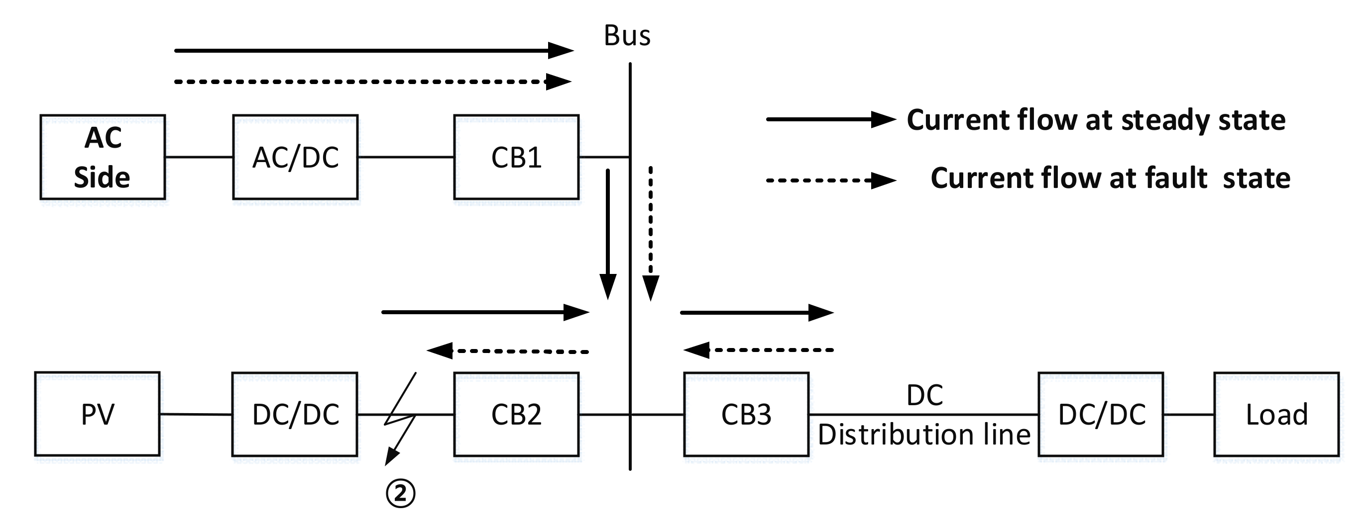
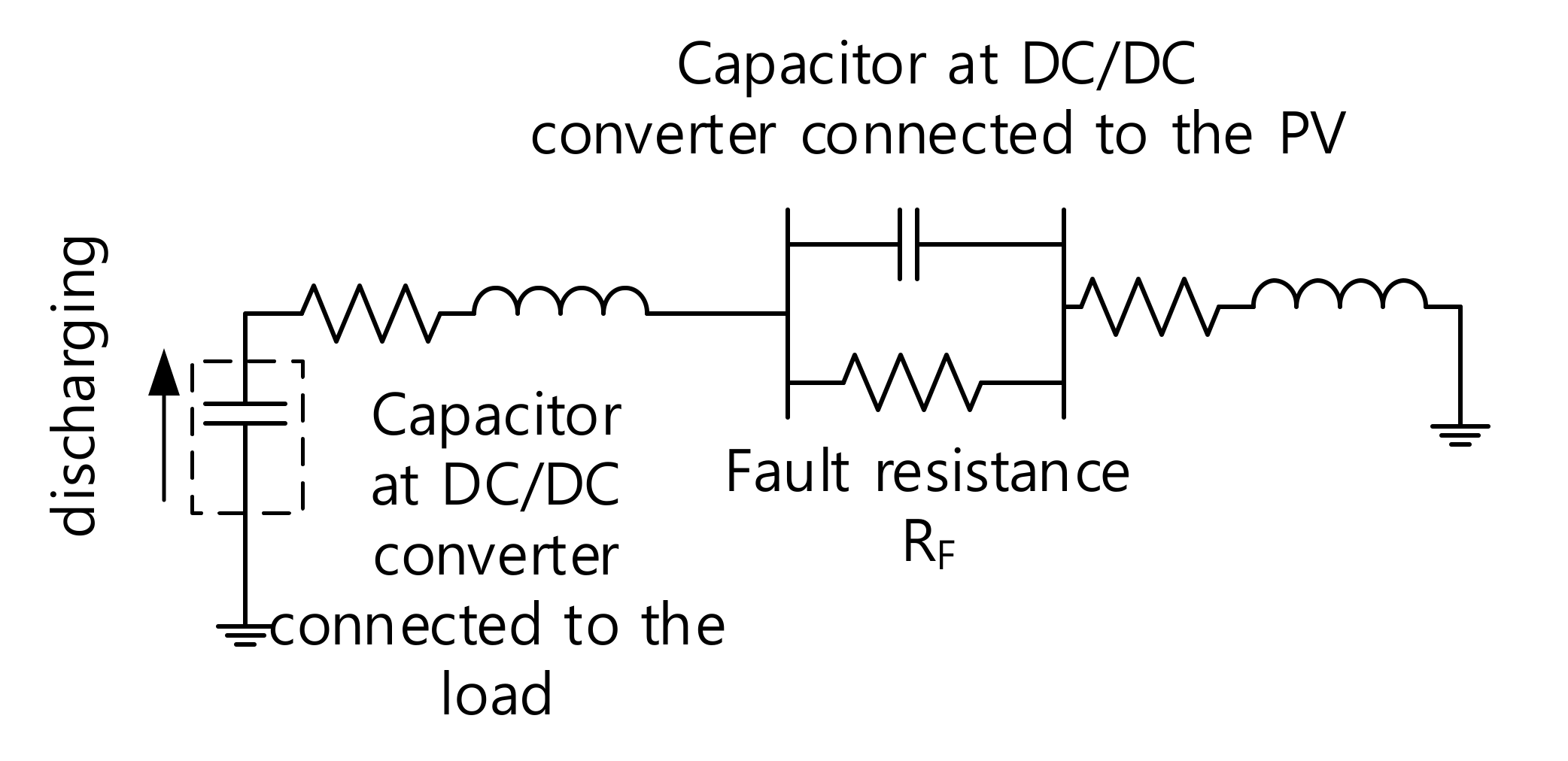
Fault section ②: Fault on the DC/DC converter connected to PV (PV side)

-

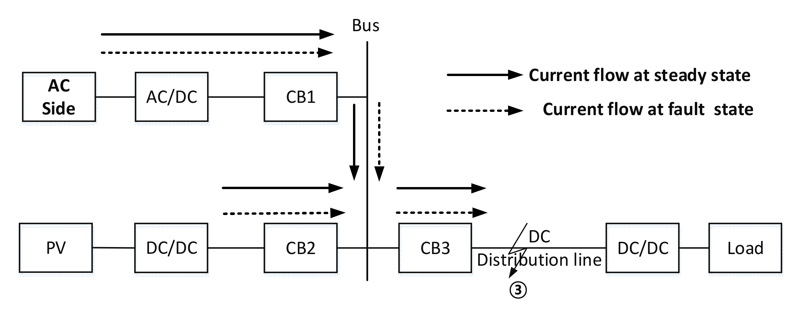
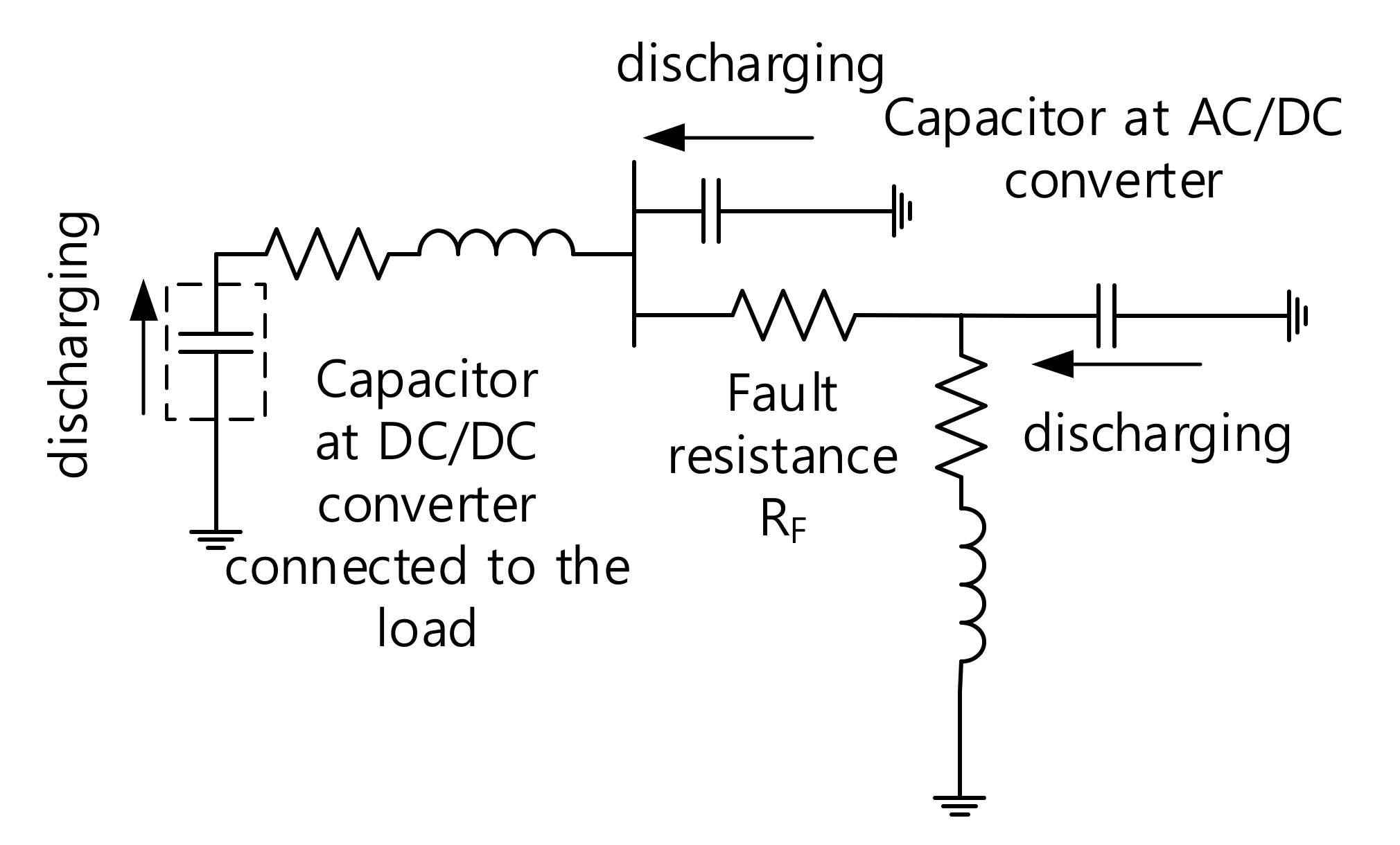
Fault section ③: Fault in DC line

-

Fault section ④: Fault in DC bus

2.1. Comparison of Direction of Steady State Current and Fault Current at Each Fault Section

Figure 2 compares the flows of currents at steady state and fault state when the fault occurs on the AC/DC converter side (fault section ①). Under a steady state, the current flows to the load. However, in CB1, the fault current flows in the opposite direction to the steady state owing to the discharge of the capacitor of the DC/DC converters connected to the PV and load. Accordingly, a current with a polarity opposite to that of the steady state flows. In CB2, the directions of current flow in the steady state and fault state are the same. In CB3, the fault current flows in the opposite direction to the steady state owing to the discharge of the capacitor of the DC/DC converter connected to the load. Figure 3 compares the current flow in the steady state and fault state in section ②. In CB1, the directions of currents in the fault state and steady state are the same. In CB2, power is supplied from the PV side to the load in the steady state, but when a fault occurs, the fault current flows in the opposite direction to the steady state owing to the capacitor discharge of the AC/DC converter and the DC/DC converter connected to the load. Thus, a current of opposite polarity will be measured. In CB3, the current flows in the opposite direction to the steady state because of the discharge of the capacitor of the DC/DC converter connected to the load, and a current of the opposite polarity will be measured. Figure 4 compares the current flow in the normal state and fault state in section ③. In CB1, CB2, and CB3, the direction of the current flow is the same in the normal and fault states. Therefore, a current with the same polarity as the steady state will be measured. Figure 5 compares the current flow in the normal state and fault state in section ④. The direction of the current measured in CB1 and CB2 is the same as that in the steady state. However, the current measured in CB3 flows in the opposite direction to the normal state owing to the discharge of the DC/DC capacitor connected to the load.

In Figure 2, Figure 3, Figure 4 and Figure 5, the flow of steady-state currents and fault currents in CB1, CB2, and CB3 are compared.

Table 1. Change of current polarity in CB1, CB2, and CB3 at each fault section.

Fault Section	CB1	CB2	CB3
①	(+) → (−)	(+) → (+)	(+) → (−)
②	(+) → (+)	(+) → (−)	(+) → (−)
③	(+) → (+)	(+) → (+)	(+) → (+)
④	(+) → (+)	(+) → (+)

summarizes the comparison of current flows. In Table 1, (+) indicates current flow in the steady-state direction. (−) indicates that the fault current flow is reversed, and the current is measured with the opposite polarity to that in the steady state.

2.2. Characteristics of Fault Current in CB1, CB2, and CB3 at Each Fault Section

At fault section ① (fault on the AC/DC converter side), the current flowing in CB1 will be the sum of CB2 and CB3. The current flowing through CB2 and CB3 is the capacitor discharge current of the DC/DC converter and can be defined as follows. Note that (–) is attached to i_CB3(1) because the direction of the current is changed, as shown in Table 1.

i_CB2(1) [A] = i_{DC/DC_PV(1)} [A] (capacitor discharge current of the DC/DC converter connected to the PV when a fault occurs in fault section ①).

i_CB3(1) [A] = −i_{DC/DC_Load(1)} [A] (capacitor discharge current of the DC/DC converter connected to the load when a fault occurs in fault section ①).

Because the current flowing through CB2 and CB3 flows into CB1, the current at CB1 can be defined as in Equation (1). Because the current direction of the fault state is opposite to that of the steady state, ($-$) is added.

i_CB1(1) [A] = −(i_CB2(1) − i_CB3(1)) = −(i_{DC/DC_PV(1)} − (−i_{DC/DC_Load(1)}))

(1)

Therefore, when a fault occurs in fault section ①, the sum of the currents flowing through CB1, CB2, and CB3 based on the steady-state direction can be calculated using Equation (2).

i_sum(1) [A] = i_CB1(1) + i_CB2(1) + i_CB3(1)
= −i_{DC/DC_PV(1)} − i_{DC/DC_Load(1)} + i_{DC/DC_PV(1)} − i_{DC/DC_Load(1)} = −2 i_{DC/DC_Load(1)}

(2)

In fault section ② (fault on the PV side), the current flowing to CB1 is the fault current supplied from the AC/DC converter, and the current flowing to CB3 is the capacitor discharge current of the DC/DC converter connected to the load. These can be defined as follows. Note that (–) is attached to I_CB3(2) because the direction of the current is changed, as shown in Table 1.

i_CB1(2) [A] = i_AC/DC(2) [A] (fault current from the AC/DC converter when fault occurs in fault section ②).

i_CB3(2) [A] = −i_{DC/DC_Load(2)} [A] (capacitor discharge current of the DC/DC converter connected to the load when fault occurs in fault section ②).

Because the current flowing through CB1 and CB3 flows into CB2, the current at CB2 can be defined by Equation (3).

i_CB2(2) [A] = −(i_CB1(2) − i_CB3(2)) = −(i_AC/DC(2) − (−i_{DC/DC_Load(2)}))

(3)

Therefore, when a fault occurs in fault section ②, the sum of the currents flowing through CB1, CB2, and CB3 based on the steady-state direction can be calculated using Equation (4).

i_sum(2) [A] = i_CB1(2) + i_CB2(2) + i_CB3(2)
= i_AC/DC(2) − (i_AC/DC(2) − (−i_{DC/DC_Load(2)})) − i_{DC/DC_Load(2)} = −i_{DC/DC_Load(2)}

(4)

In fault section ③ (DC line fault), the current flowing through CB1 is the fault current supplied from the AC/DC converter. The current flowing through CB2 is the capacitor discharge current of the DC/DC converter connected to the PV. The above two parameters can be defined as follows:

i_CB1(3) [A] = i_AC/DC(3) [A] (fault current from AC/DC converter when fault occurs in fault section ③).

i_CB2(3) [A] = i_{DC/DC_PV(3)} [A] (capacitor discharge current of the DC/DC converter connected to the PV when fault occurs in fault section ③).

The current flowing through CB3 is the sum of the currents flowing through CB1 and CB2, as shown in Equation (5).

i_CB3(3) [A] = i_CB1(3) + i_CB2(3) = i_AC/DC(3) + i_{DC/DC_PV(3)}

(5)

Therefore, when a fault occurs in fault section ③, the sum of the currents flowing through CB1, CB2, and CB3 based on the steady-state direction can be calculated using Equation (6).

i_sum(3) [A] = i_CB1(3) + i_CB2(3) + i_CB3(3) = 2(i_AC/DC(3) + i_{DC/DC_PV(3)})

(6)

In fault section ④ (DC bus fault), the current flowing through CB1 is the fault current supplied from the AC/DC converter. The current flowing through CB2 is the capacitor discharge current of the DC/DC converter connected to the PV, and the current flowing through CB3 is the capacitor discharge current of the DC/DC converter connected to the load. The three parameters above can be defined as follows.

i_CB1(4) [A] = i_AC/DC(4) [A] (Fault current from AC/DC converter when a fault occurs in fault section ④).

i_CB2(4) [A] = i_{DC/DC_PV(4)} [A] (capacitor discharge current of the DC/DC converter connected to the PV when a fault occurs in fault section ④).

i_CB3(4) [A] = −i_{DC/DC_Load(4)} [A] (capacitor discharge current of the DC/DC converter connected to the load when a fault occurs in fault section ④).

Therefore, when a fault occurs in fault section ④, the sum of the currents flowing through CB1, CB2, and CB3 based on the steady-state direction can be calculated using Equation (7).

i_sum(4) [A] = i_CB1(4)+ i_CB2(4)+ i_CB3(4) = i_AC/DC(4) + i_{DC/DC_PV(4)} − i_{DC/DC_Load(4)}

(7)

Based on the formulae derived above, we analyzed the harmonic and high-frequency components.

First, comparing the sum of the currents flowing through each CB at the four fault sections, it can be seen that (2) and (4) consist of only the capacitor discharge current of the DC/DC converter, and (6) and (7) consist of the fault current from the AC/DC converter and the capacitor discharge current of the DC/DC converter. In the case of the fault current supply from the AC/DC converter, because the current supplied from the six-pulse diode rectifier is included, the currents in (6) and (7) will contain more harmonics and high-frequency components than the current calculated in (2) and (4). In other words, it can be predicted that the fault in the DC line and the fault in the DC bus will contain more harmonics and high frequencies than the fault on the AC/DC converter side and the fault on the PV side.

As a next step, we compared the harmonics and high-frequency components of faults in the DC lines and faults in the DC bus. In (6), the fault current from the AC/DC converter and the capacitor discharge current of the DC/DC converter are included. In (7), because the capacitor discharge current part of the DC/DC converter consists of two quantities subtracted from each other, it is judged that these cancel each other out. In (6), because the fault current from the AC/DC converter and the capacitor discharge current are summed, it is impossible to predict whether the contents of harmonics and high-frequency components increase or decrease. That is, it is unpredictable whether the harmonic and high-frequency components are greater in the faults in the DC lines or in the DC bus.

As a final step, we analyzed the faults on the AC/DC converter side and on the PV side. In the view of the DC/DC converter connected to the load, the capacitor of the DC/DC converter connected to the PV is included in the current flow path when the fault on the AC/DC converter side occurs; however, it is not included when the fault on the PV side occurs. The equivalent circuit for each fault condition is shown in Figure 6 and Figure 7.

In Figure 6, the equivalent impedance from the capacitor side of the DC/DC converter connected to the load is given by Equation (8).

$$Z_{\left(1\right)}\left[\mathsf{\Omega }\right]=2\left(R+j\omega L\right)+\left(R_F//-j{X}_c\right)$$

(8)

In Figure 7, the equivalent impedance from the capacitor side of the DC/DC converter connected to the load is given by Equation (9).

$$Z_{\left(2\right)}\left[\mathsf{\Omega }\right]=2\left(R+j\omega L\right)+R_F$$

(9)

Comparing the magnitudes of (8) and (9), $2\left(R+j\omega L\right)$ is the same, and hence, the magnitude is determined by the other terms. In (8), the magnitude of $\left(R_F//-j{X}_c\right)$ is given by (10).

$$\left|Z_{\left(2\right)\_parallel}\right|\left[\mathsf{\Omega }\right]=\frac{R_F{X}_C}{\sqrt{R_F^2+X_C^2}}$$

(10)

To compare the magnitudes of (9) and (10), the difference between the two equations is calculated using (11). In (11), $\sqrt{R_F^2+X_C^2}-X_C$ is larger than 0, except when $R_F$ = 0, and (9) is larger than (10). In other words, (9) is larger than (8).

$$R_F-\frac{R_F{X}_C}{\sqrt{R_F^2+X_C^2}}=\frac{R_F\left(\sqrt{R_F^2+X_C^2}-X_C\right)}{\sqrt{R_F^2+X_C^2}}$$

(11)

In view of the capacitor of the DC/DC converter connected to the load, the equivalent impedance at the fault on the PV side is larger than that of the fault on the AC/DC converter side. Accordingly, the discharging current of the capacitor of the DC/DC converter connected to the load will have a larger value in the case of a fault on the AC/DC converter side. That is, when comparing (2) and (4), which is the sum of the three CB currents at each fault, the value of (2) will be larger. The capacitor discharge current in the DC system is not a constant value, and is attenuated according to a time constant. Assuming that the time constants are similar in both cases, it is predicted that a larger discharge current value contains more harmonics and high-frequency components. In other words, it is predicted that the faults on the AC/DC converter side have greater harmonic and high-frequency components than the faults on the PV side.

Summarizing the above analysis results, the order in which more harmonics and high-frequency components occur is line fault (fault ③) and bus fault (fault ④), AC/DC converter side fault (fault ①), and PV side fault (fault ②).

3. Development of New Protection Scheme in DC Microgrid Using Wavelet Transform

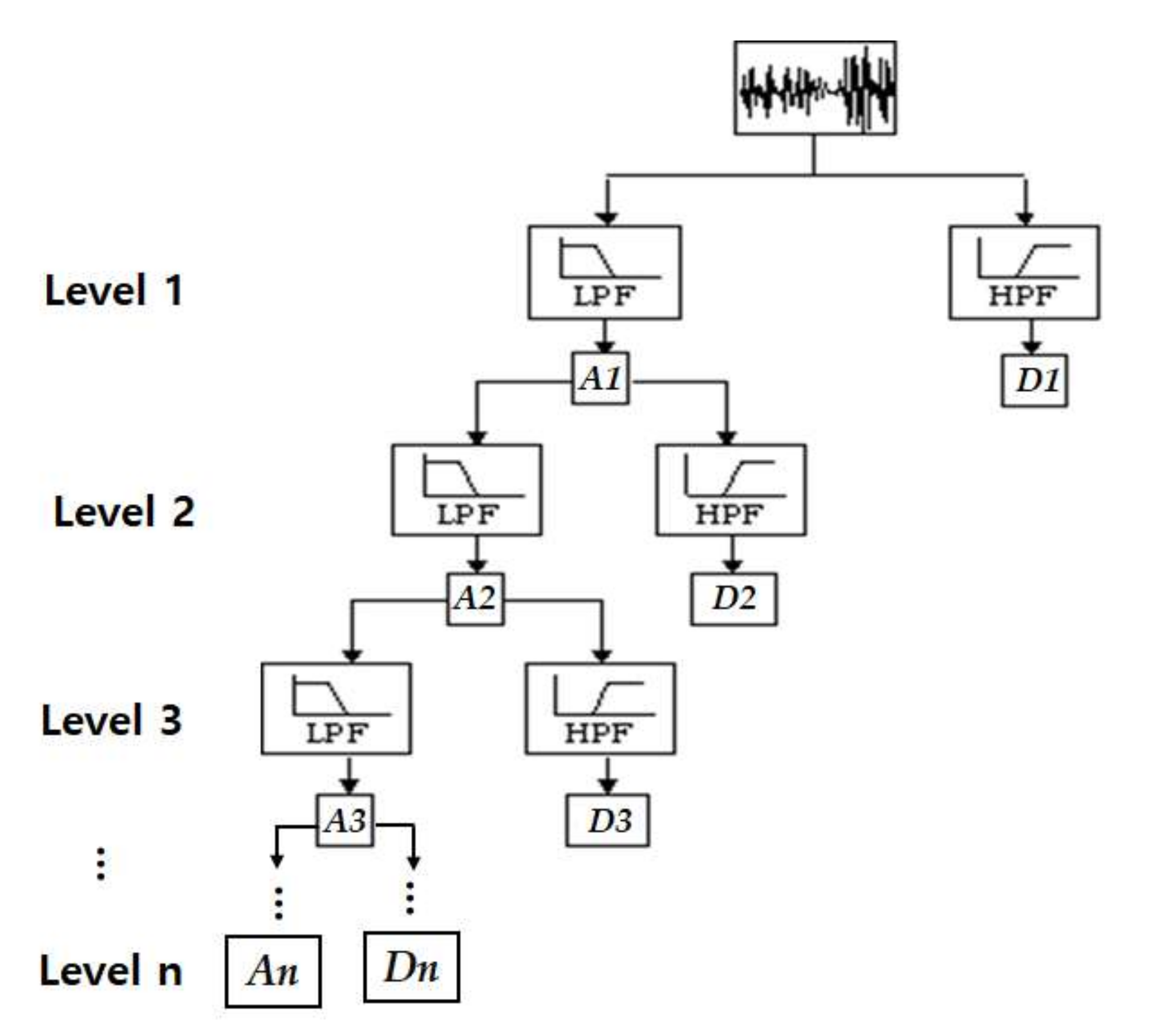
3.1. Wavelet Transform

A WT can extract time and frequency information simultaneously from an original signal [28]. The discrete wavelet transform (DWT) of a signal is defined as:

$$DWT\left(m,k\right)=\frac{1}{\sqrt{a_0^m}}{{\displaystyle \sum }}_{k=1}^{N}x\left(n\right)g\left(\frac{k-n{a}_0^m{b}_0}{a_0^m}\right)$$

(12)

where $x(n)$ is the input signal, $g(n)$ is the mother wavelet, k is the present sample, $a_0^m$ is a scale parameter, $n{a}_0^m{b}_0^{}$ is the time shift of $g(n)$, and translation parameter $b_0$ is function of integer parameter $m$.

After performing the WT, the original signal decomposed to the detail (D) component and approximation (A) components. The detail component represents the high-frequency components of a signal and the approximation components represents the low-frequency components of a signal. The approximation can be decomposed many times with detail and approximation as shown in Figure 8. In Figure 8, level n means the numbers of approximation decomposed when the WT is performed. An and Dn mean the approximation coefficient and the detail coefficient at level n. In this process, the original signal S can be represented as follows [28]:

S = D1 + D2 + ⋯ + Dn + An

(13)

There are various mother wavelets, such as Haar, Daubechies (db) N, and Symlets N that can be used for WT. The mother wavelets are classified according to its length and properties and they have different characteristics. For example, the db mother wavelet has asymmetric basic functions, while the Sym mother wavelet has the least asymmetric basic functions. In signal processing, the WT can be obtained by scaling and moving the mother wavelet. Therefore, it is very important to select an appropriate mother wavelet [26,27,28].

3.2. System Configuration

The system configuration of the proposed new protection method in the LVDC microgrid is shown in Figure 9. The protection relay receives the current flowing through each breaker as an input and sends a trip signal to each breaker. Communication technology is used to transmit input/output signals.

3.3. New Protection Scheme in DC Microgrid Using Wavelet Transform

Figure 10 shows a flowchart of the proposed method. The proposed method first receives the DC currents (i₁ [A], i₂ [A], i₃ [A]) flowing through each CB as input, and then determines whether a fault has occurred. If the input currents are greater than the fault judgement current (i_fault [A]), it is judged to be a fault, and the sum of the three currents (i_sum [A]) is calculated. Because i₁, i₂, and i₃ are DC currents, the i_sum is obtained by summing only the algebraic magnitudes.

Among the various mother wavelets, db4 has been widely used for power system transients and protection. Therefore, in this study, the mother wavelet has also been selected as db4, and the detailed components are taken after performing two WTs at levels 2 and 8. After the WTs, (14) and (15) are calculated using detail components. In (14) and (15), D2 and D8 are the detailed components after the WTs. T is the period (16.66 ms) based on an AC frequency of 60 Hz. This paper is based on the 120 samples/cycle. In (14) and (15), s means the present sample and s − 120 means the sample before 1 cycle. (14) and (15) mean the rms value of D2 and D8 components.

$$I_{wave\_rms1}\left(t\right)=\sqrt{\frac{1}{T}{{\displaystyle \int }}_{s-120}^{s}D{2}^2 dt}$$

(14)

$$I_{wave\_rms2}\left(t\right)=\sqrt{\frac{1}{T}{{\displaystyle \int }}_{s-120}^{s}D{8}^2 dt}$$

(15)

The trip commands of CBs are issued after determining the fault section using this value. Based on this analysis, WT can be performed to determine the fault section. As the level at WT increases, more harmonics and high-frequency parts can be extracted, and this result is included in the detailed component.

Using (14), it is primarily determined whether there is a line fault (fault ③), bus fault (fault ④), AC/DC converter side fault (fault ①) or PV side fault (fault ②). In the algorithm shown in Figure 9, α is a threshold value used to distinguish between the fault types. If the result of (14) is less than this value, it is judged as an AC/DC converter side fault or PV side fault, and if it is larger than this value, it is judged as a DC line fault or bus fault.

After dividing the fault sections into two parts, it is necessary to classify the failure types into pole-to-pole (ptp) and pole-to-ground (ptg) faults. This is because the same threshold value cannot be applied because the fault current in the ptp fault is larger than the fault current in the ptg fault owing to the capacitor discharge current characteristics.

If an AC/DC side fault or PV side fault is predicted, determination of a ptp fault or ptg fault is predicted using (15). Because the fault current is larger in a ptp fault, the value of (15) is also expected to be larger in a ptp fault. γ is a threshold value for predicting ptp and ptg faults in the case of AC/DC or PV faults. If I_{wave_rms2}(t) > γ is satisfied, it is predicted to be a ptp fault, and the condition of I_{wave_rms1}(t) > β1 is applied. If I_{wave_rms2}(t) > γ is not satisfied and it is predicted to be a ptg fault, the condition of I_{wave_rms1}(t) > β2 is applied. β1 and β2 are threshold values for judging AC/DC side or PV side faults. If the value of Iwave_rms1 is smaller than β1 or β2 according to each condition, it is judged as a PV side fault, only CB2 is opened to block the fault section, and the rest are kept closed. Through this operation, there is an advantage that power can be continuously supplied from the AC side to the load side. If the value of Iwave_rms1 is greater than β1 or β2, it is judged as a fault on the AC/DC side and only CB1 is opened and the rest are kept closed, so that the power supply from the PV side to the load can be continued.

When it is determined whether there is a line fault or a bus fault, WT is not applied because harmonics and high-frequency content cannot be predicted when classifying two fault sections. In this case, the fault section can be determined simply by applying Equation (5). (5) is the concept of differential protection applied to busbar protection. If (5) is satisfied, it is judged to be a line fault, and if not satisfied, it is judged to be a bus fault. In the case of a DC line fault, only CB3 is opened. Operations, such as reverse power transmission to the AC side or ESS charging, can then be performed from the PV. In the case of a DC bus fault, all circuit breakers are opened to cut off the continuous supply of the fault current.

The threshold values α, β1, β2, and γ for fault area determination are variable and depend on various factors, such as system configuration, load capacity, and PV capacity. These values can be set through simulations of various cases according to the fault section, fault resistance, fault distance, and fault type in the system to which the algorithm proposed in this paper is applied. Through this process, α was set to 500, β1 was set to 250, β2 was set to 100, and γ was set to 8000. If the proposed algorithm is applied to other LVDC distribution system, the threshold values α, β1, β2, and γ should also be changed for the applied LVDC distribution system.

4. Simulations

4.1. System Model

The system model used to verify the proposed method is shown in Figure 9. The AC source is assumed as a power source with large capacity to deliver the power from the substation to the load. The PV capacity was 2 kW. The length of the DC distribution line was 2 km, and the DC load was 50 kW.

The system model was implemented using the EMTP/ATPDraw. A detailed control operation of the AC/DC converter and DC/DC converter was implemented using EMTP/MODELS. The proposed algorithm in Figure 10 was implemented using MATLAB.

4.2. Simulation Conditions

Table 2. Simulation conditions.

Case	Fault Section	Fault Type	Fault Resistance (ohm)	Fault Distance
1	AC/DC converter side	Pole-to-Pole	0.1	-
2	PV side	Pole-to-Pole	0.1	-
3	DC Line side	Pole-to-Pole	0.1	20%
4	DC Line side	Pole-to-Pole	0.1	50%
5	DC Line side	Pole-to-Pole	0.1	80%
6	DC Bus side	Pole-to-Pole	0.1	-
7	AC/DC converter side	Pole-to-ground	0.1	-
8	PV side	Pole-to-ground	0.1	-
9	DC Line side	Pole-to-ground	0.1	20%
10	DC Line side	Pole-to-ground	0.1	50%
11	DC Line side	Pole-to-ground	0.1	80%
12	DC Bus side	Pole-to-ground	0.1

lists the simulation conditions used to verify the proposed method. The fault sections were set to the AC/DC converter side, PV side, DC line side, and DC bus side. Each fault section is illustrated in Figure 1. Fault types were set as ptp faults (Cases 1–6) and ptg faults (Cases 7–12). The fault resistance was the same in all Cases, and was set as a low-resistance fault. In the case of a line fault, the fault distance was varied between 20%, 50%, and 80%. The fault occurred at 0.5 s, and the fault duration was set as a permanent fault.

4.3. Simulation Results and Discussion

The meanings of the fault sections and CB operations for each simulation waveform are presented in

Table 3. Meanings of the fault sections and CB operations.

Fault Section		CB Operation
0	Non-fault	0	open
1	AC/DC side fault	1	CB1 close
2	PV side fault	2	CB2 close
3	DC Line fault	3	CB3 close
4	DC Bus fault

.

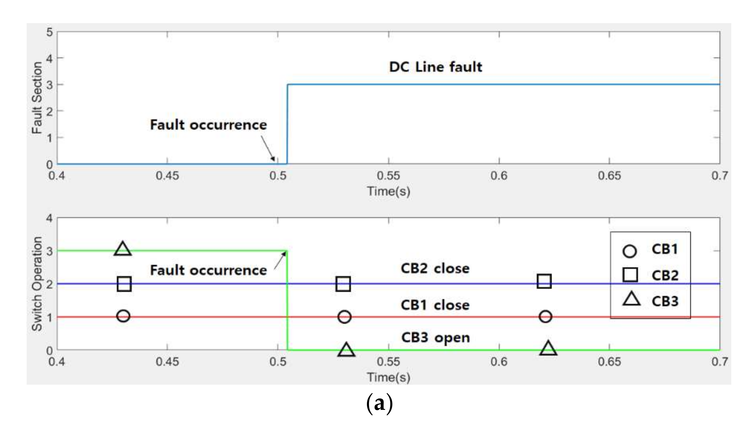
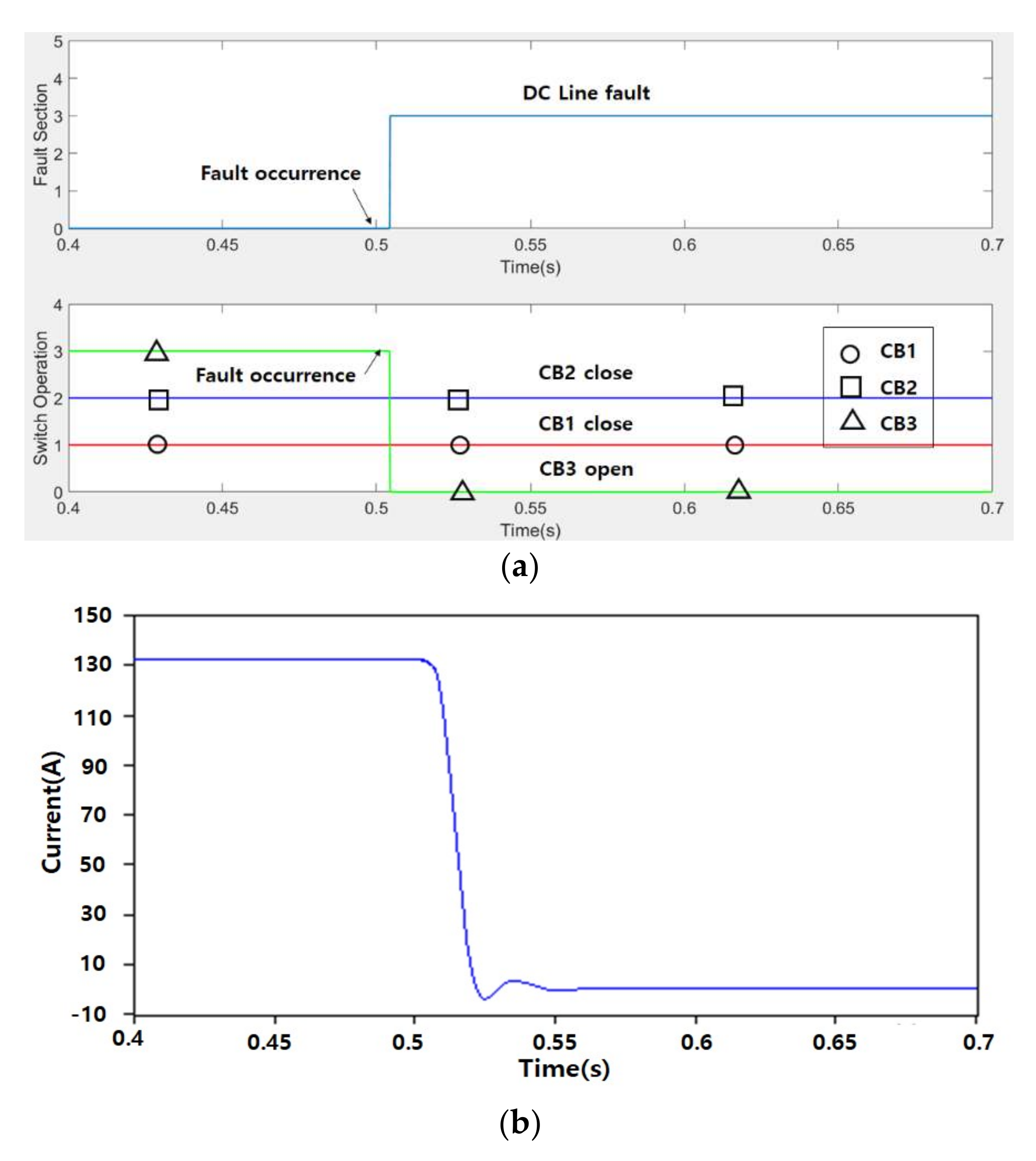
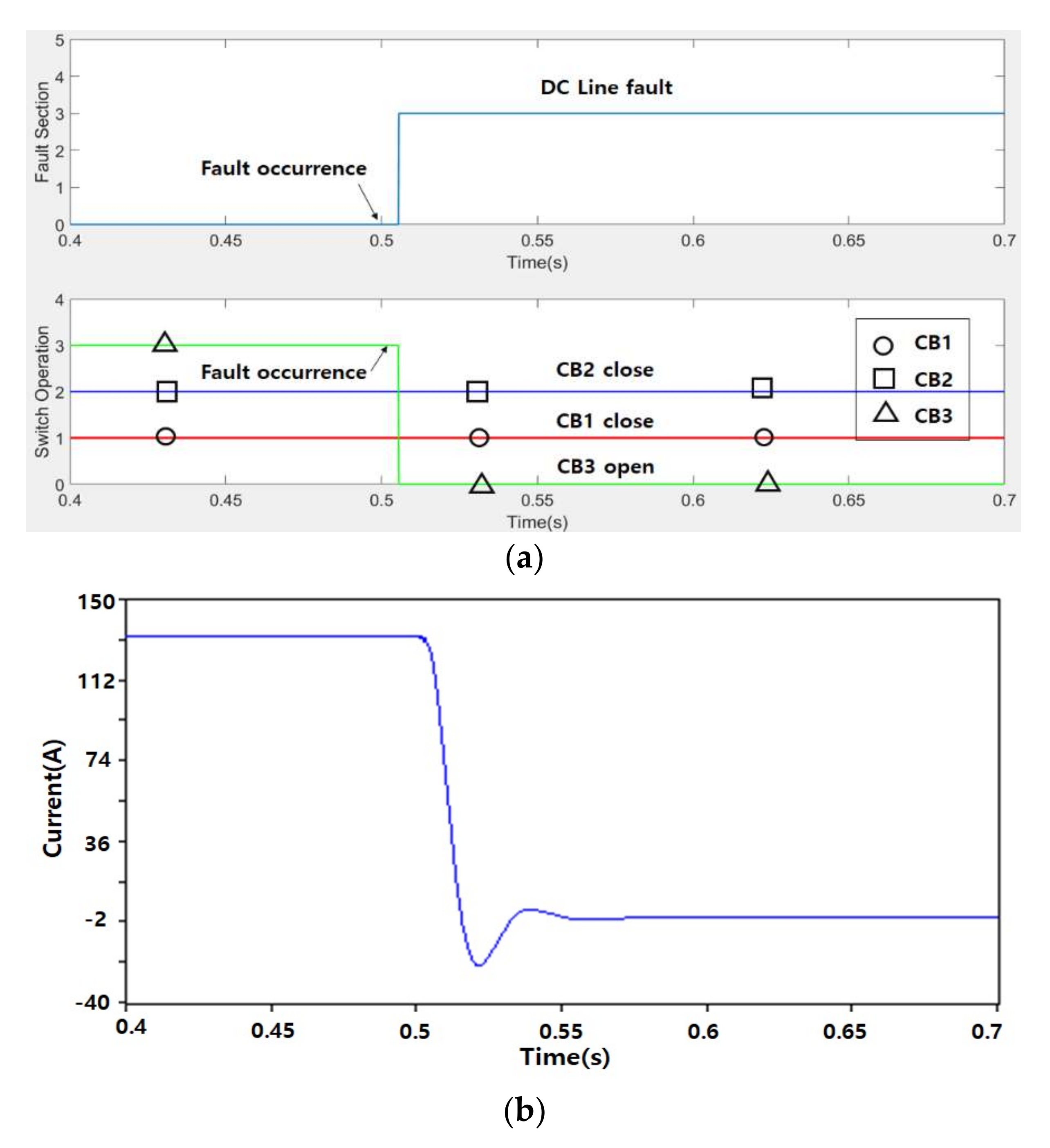
4.3.1. Simulation Results of Cases 1–6

Cases 1–6 are cases of ptp faults.

Table 4. Maximum value of I_{wave_rms1}(t) and I_{wave_rms2}(t) at Cases 1–6.

Case	Maximum Value of Iwave_rms1(t)	Maximum Value of Iwave_rms2(t)
Case 1	460	11,800
Case 2	199	13,930
Case 3	1394
Case 4	848
Case 5	549
Case 6	900

shows the maximum value of I_{wave_rms1}(t) and I_{wave_rms2}(t) calculated by simulations at Cases 1–7. I_{wave_rms2}(t) in Cases 3–6 are not presented because this value is not used to judge the fault section in Cases 3–6. In these Cases, a comparison of I_{wave_rms1}(t) calculated by (14) in Cases 1, 2, 4, and 6 is shown in Figure 11. Cases 3 and 5 are not presented because Case 4 is a representative case of DC line faults. Among the conditions in Figure 10, according to the condition of I_{wave_rms1}(t) < α (=500), Cases 1 and 2 are judged to be AC/DC side faults or PV side faults, and Cases 4 and 6 are DC line faults or DC bus faults. Figure 12 compares I_{wave_rms2}(t) for Cases 1 and 2. A fault occurs at 0.5 s, the condition of I_{wave_rms2}(t) > γ (=8000) is satisfied before 0.51 sec, which is the time when the transient is present, and it is judged as a ptp fault.

Figure 13a shows the fault section and CB operation in Case 1. According to the proposed algorithm, the fault section is determined to be the AC/DC side (fault section ①), and only CB1 performs an open operation at 0.5042 s. Figure 13b shows the load current in Case 1. Despite the occurrence of a fault, it can be seen that the normal current flows continuously in the load owing to the PV and load-side capacitor discharge because of the blocking of the fault current injection by the proposed algorithm. Figure 14 shows the simulation results for Case 2. In this case, the fault section is accurately predicted according to the proposed algorithm as a fault on the PV side (fault section ②), and accordingly, CB2 opens at 0.5068 s. From the load current in Figure 14b, it can be seen that the normal current is continuously flowing without blackout or transient because the normal current is injected from the AC/DC converter side.

Figure 15, Figure 16 and Figure 17 show the results of Cases 3–5, which are cases of DC line faults. The difference in Cases 3–5 is the fault distance. As shown in Figure 15a, Figure 16a and Figure 17a, from the simulation results, the fault section is accurately judged as section ③, and only CB3 is opened at 0.5042, 0.5043, and 0.5052 s according to the proposed algorithm. Figure 15b, Figure 16b and Figure 17b show the load current in Cases 3–5. From these figures, it can be seen that the fault still remains even after CB3 is opened, so the discharge current of the capacitor flows to the fault point and no normal current flows in the load.

Figure 18 shows the simulation results for Case 6. As the fault section is shown as ④, it is accurately judged as a DC bus fault, and therefore all CBs are opened. It can be seen that although the normal current is initially supplied to the load owing to the discharge of the load-side capacitor, the current value gradually decreases thereafter.

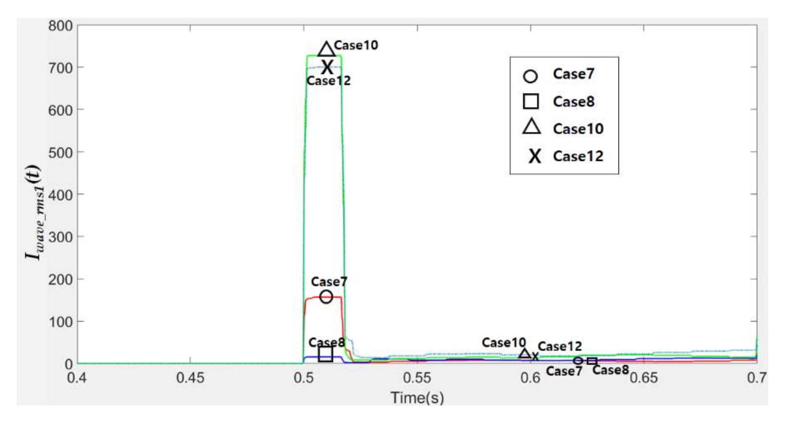
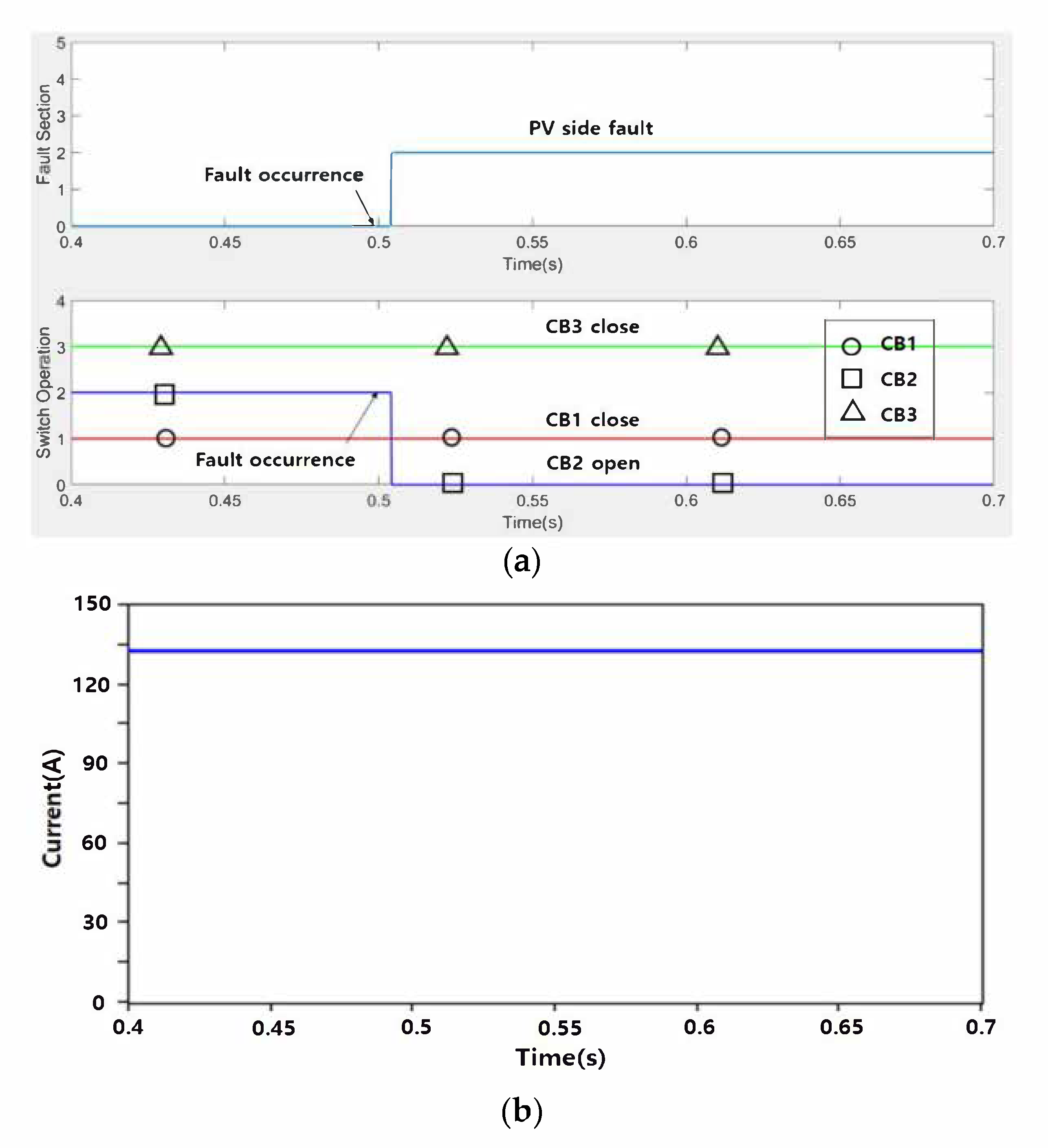
4.3.2. Simulation Results in Cases 7–12

Table 5. Maximum value of I_{wave_rms1}(t) and I_{wave_rms2}(t) at Cases 7–12.

Case	Maximum Value of Iwave_rms1(t)	Maximum Value of Iwave_rms2(t)
Case 7	164	4500
Case 8	27	1920
Case 9	1085
Case 10	727
Case 11	537
Case 12	700

shows the maximum value of I_{wave_rms1}(t) and I_{wave_rms2}(t) in Cases 7–12. I_{wave_rms2}(t), in Cases 9–12, are not presented because this value is not used to judge the fault section. Figure 19 compares the calculation results of I_{wave_rms1}(t) in Cases 7, 8, 10, and 12. The four cases are representative cases according to the fault sections for ptg faults. The algorithm uses the condition of I_{wave_rms1}(t) < α (=500) to determine whether AC/DC side or PV side faults, DC line side faults, or bus faults exist. Because the maximum values of I_{wave_rms1}(t) in Cases 10 and 12 are larger than α as shown in Figure 19 and Table 5, they are judged to be DC line or bus faults. Because the maximum values of I_{wave_rms1}(t) in Cases 7 and 8 are smaller than α as shown in Figure 19 and Table 5, they are judged to be AC/DC side or PV side faults. The judgement of ptp or ptg fault is determined according to the result of I_{wave_rms2}(t) in Figure 20. In Figure 20, these values do not satisfy the condition of I_{wave_rms2}(t) > γ (=8000), so the faults are determined as ptg failures. Therefore, the condition I_{wave_rms1}(t) < β2 (=100) is applied to determine the fault section, and the CB operation is determined.

Figure 21 shows the simulation results for Case 7. Because I_{wave_rms1}(t) is greater than 100, it is judged to be an AC/DC side fault, so the fault section is 1 in the simulation result, and accordingly, only CB1 is opened at 0.5051 s. It can be seen that the normal current is continuously supplied to the load current owing to the capacitor discharge of the DC/DC converter connected to the PV and load.

Figure 22 shows the simulation results for Case 8. Because I_{wave_rms1}(t) is less than 100, it is judged as a PV-side fault, and only CB2 is opened at 0.504 s. It can also be seen that the normal load current is supplied through the AC/DC converter from the AC side.

Figure 23, Figure 24 and Figure 25 show the simulation results of Cases 9–11, which are cases of DC line faults. As shown in Figure 23a, Figure 24a and Figure 25a, it can be seen that the fault section was accurately determined as DC line fault (fault section ③) according to the proposed algorithm, and only CB3 opened at 0.504, 0.5043, and 0.505 s, respectively. After CB3 opened, because a ptg fault occurred, only one of the two polarities of the DC line is in a fault state, and the other polarity is in the normal state. Therefore, it can be seen that a normal current in Figure 23b, Figure 24b and Figure 25b is initially supplied to the load current due to capacitor discharge, but the current value gradually decreases thereafter.

Figure 26 shows the simulation results for Case 12. From the simulation results, it can be seen that all CBs are opened by determining the DC bus fault. As with the result of Case 6, it can be seen that although the normal current is initially supplied to the load current owing to the capacitor discharge, the current value gradually decreases thereafter.

In the simulation results, a comparison with any previous method was not performed. This is because a previous conventional method has not been established, and the results of previous studies determining the fault section and studying the CB operation also do not exist.

5. Conclusions

In this paper, a new protection method is proposed using wavelet transform in an LVDC microgrid. First, the fault section in the LVDC microgrid was divided into four areas: AC/DC converter side, PV side, DC line side, and DC bus side, and the direction and characteristics of the fault current were analyzed at each fault section. Based on these analyses, a new protection method was proposed using the WT in an LVDC microgrid. The proposed method receives currents from three CBs located on an LVDC microgrid as input and calculates the sum of these currents. Using this value, WT at levels 2 and 8 with db4 as the mother wavelets is performed, and I_{wave_rms1}(t) and I_{wave_rms2}(t) are calculated by (14) and (15) using detail coefficients. Using these values, the fault sections (AC/DC converter side, PV side, DC line side, and DC bus side) were determined, and the CB operations were determined for each fault section.

To verify the proposed method, an LVDC microgrid was modelled using the EMTP/ATPDraw, and the proposed algorithm was implemented using MATLAB. Various simulations were performed according to the fault sections and fault types. The simulation results showed that the fault section was accurately determined, and the corresponding CB operations were performed.

The method performed in this study is suitable only for low-impedance fault cases. In the future, we will develop a protection method that considers high-resistance faults in an LVDC microgrid.

References

1. Elia, S.; Santantonio, A. Fire Risk in MTBF Evaluation for UPS System. Adv. Electr. Electron. Eng. 2016, 14, 189–194. [Google Scholar] [CrossRef]
2. Elia, S.; Santini, E.; Tobia, M. Comparison between Different Electrical Configurations of Emergency Diesel Generators for Redundancy and Reliability Improving. Period. Polytech. Electr. Eng. Comput. Sci. 2018, 62, 144–148. [Google Scholar] [CrossRef] [Green Version]
3. Bracci, D.; Elia, S.; Ruvio, A. A study on a high-reliability electromechanical undervoltage relay immersed in natural ester oil: Application in mutual aid system for gensets using. In Proceedings of the IEEE International Conference on Dielectric Liquids ICDL 2019, Rome, Italy, 23–27 June 2019. [Google Scholar]
4. Boccaletti, C.; Elia, S.; Salas, M.E.F.; Pasquali, M. High reliability storage systems for genset cranking. J. Energy Storage 2020, 29, 101336. [Google Scholar] [CrossRef]
5. D’Orazio, A.; Elia, S.; Santini, E.; Tobia, M. Succor System and Failure Indication for the Starter Batteries of Emergency Gensets. Period. Polytech. Electr. Eng. Comput. Sci. 2020, 64, 412–421. [Google Scholar] [CrossRef]
6. Emhemed, A.A.S.; Burt, G.M. An Advanced Protection Scheme for Enabling an LVDC Last Mile Distribution Network. IEEE Trans. Smart Grid 2014, 5, 2602–2609. [Google Scholar] [CrossRef] [Green Version]
7. Emhemed, A.A.S.; Fong, K.; Fletcher, S.; Burt, M.G. Validation of Fast and Selective Protection Scheme for an LVDC Distribution Network. IEEE Trans. Power Deliv. 2017, 32, 1432–1440. [Google Scholar] [CrossRef] [Green Version]
8. Shamsoddini, M.; Vahidi, B.; Razani, R.; Nafisi, H. Extending protection selectivity in low voltage DC microgrids using compensation gain and artificial line inductance. Electr. Power Syst. Res. 2020, 188, 106530. [Google Scholar] [CrossRef]
9. Noh, C.-H.; Kim, C.-H.; Gwon, G.-H.; Khan, M.O.; Jamali, S.Z. Development of protective schemes for hybrid AC/DC low-voltage distribution system. Int. J. Electr. Power Energy Syst. 2019, 105, 521–528. [Google Scholar] [CrossRef]
10. Ravyts, S.; Broeck, G.V.d.; Hallemans, L.; Vecchia, M.D.; Driesen, J. Fuse-Based Short-Circuit Protection of Converter Controlled Low-Voltage DC Grids. IEEE Trans. Power Electron. 2020, 35, 11694–11706. [Google Scholar] [CrossRef]
11. Saleh, K.A.; Hooshyar, A.; El-Saadany, E.F. Hybrid Passive-Overcurrent Relay for Detection of Faults in Low-Voltage DC Grids. IEEE Trans. Smart Grid 2017, 8, 1129–1138. [Google Scholar] [CrossRef]
12. Shamsoddini, M.; Vahidi, B.; Razani, R.; Mohamed, Y.A.R.I. A novel protection scheme for low voltage DC microgrid using inductance estimation. Int. J. Electr. Power Energy Syst. 2020, 120, 105992. [Google Scholar] [CrossRef]
13. Oh, Y.-S.; Kim, C.-H.; Gwon, G.H.; Noh, C.H.; Bukhari, S.B.A.; Haider, R.; Gush, T. Fault detection scheme based on mathematical morphology in last mile radial low voltage DC distribution networks. Int. J. Electr. Power Energy Syst. 2019, 106, 520–527. [Google Scholar] [CrossRef]
14. Jamali, S.Z.; Bukhari, S.B.A.; Khan, M.O.; Mehmood, K.K.; Mehdi, M.; Noh, C.-H.; Kim, C.-H. A High-Speed Fault Detection, Identification, and Isolation Method for a Last Mile Radial LVDC Distribution Network. Energies 2018, 11, 2901. [Google Scholar] [CrossRef] [Green Version]
15. Salehi, M.; Taher, S.A.; Sadeghkhani, I.; Shahidehpour, M. A Poverty Severity Index-Based Protection Strategy for Ring-Bus Low-Voltage DC Microgrids. IEEE Trans. Smart Grid 2019, 10, 6860–6869. [Google Scholar] [CrossRef]
16. Bhargav, R.; Bhalja, B.R.; Gupta, C.P. Novel Fault Detection and Localization Algorithm for Low-Voltage DC Microgrid. IEEE Trans. Ind. Inform. 2020, 16, 4498–4511. [Google Scholar] [CrossRef]
17. Noh, C.; Kim, C.; Gwon, G.; Oh, Y. Development of fault section identification technique for low voltage DC distribution systems by using capacitive discharge current. J. Mod. Power Syst. Clean Energy 2018, 6, 509–520. [Google Scholar] [CrossRef] [Green Version]
18. Wang, D.; Emhemed, A.; Burt, G. A novel protection scheme for an LVDC distribution network with reduced fault levels. In Proceedings of the IEEE Second International Conference on DC Microgrids (ICDCM), Nuremburg, Germany, 27–29 June 2017. [Google Scholar]
19. Lee, J.-W.; Kim, W.-K.; Oh, Y.-S.; Seo, H.-C.; Jang, W.-H.; Kim, Y.S.; Park, C.-W.; Kim, C.-H. Algorithm for Fault Detection and Classification Using Wavelet Singular Value Decomposition for Wide-Area Protection. J. Electr. Eng. Technol. 2015, 10, 729–739. [Google Scholar] [CrossRef] [Green Version]
20. Bhuvnesh, R.; Shaik, A.G. Wavelet-alienation based protection scheme for multi-terminal transmission line. Electr. Power Syst. Res. 2018, 161, 8–16. [Google Scholar]
21. Adly, A.R.; Aleem, S.H.A.; Algabalawy, M.A.; Jurado, F.; Ali, Z.M. A novel protection scheme for multi-terminal transmission lines based on wavelet transform. Electr. Power Syst. Res. 2020, 183, 106286. [Google Scholar] [CrossRef]
22. Leal, M.M.; Costa, F.B.; Campos, J.T.L.S. Improved traditional directional protection by using the stationary wavelet transform. Int. J. Electr. Power Energy Syst. 2019, 105, 59–69. [Google Scholar] [CrossRef]
23. Gautam, N.; Ali, S.; Kapoor, G. Detection of fault in series capacitor compensated double circuit transmission line using wavelet transform. In Proceedings of the International Conference on Computing, Power and Communication Technologies (GUCON), Greater Noida, India, 28–29 September 2018. [Google Scholar]
24. Gururaja Rao, H.V.; Prabhu, N.; Mala, R.C. Wavelet transform-based protection of transmission line incorporating SSSC with energy storage device. Electr. Eng. 2020, 102, 1–12. [Google Scholar] [CrossRef]
25. Mishra, D.P.; Samantaray, S.R.; Joos, G.A. Combined Wavelet and Data-Mining Based Intelligent Protection Scheme for Microgrid. IEEE Trans. Smart Grid 2016, 7, 2295–2304. [Google Scholar] [CrossRef]
26. Seo, H.C. New Protection Scheme Based on Coordination with Tie Switch in an Open-Loop Microgrid. Energies 2019, 12, 4756. [Google Scholar] [CrossRef] [Green Version]
27. Seo, H.C. Novel Protection Scheme considering Tie Switch Operation in an Open-Loop Distribution System using Wavelet Transform. Energies 2019, 12, 1725. [Google Scholar] [CrossRef] [Green Version]
28. Seo, H.C.; Rhee, S.B. Novel adaptive reclosing scheme using wavelet transform in distribution system with battery energy storage system. Int. J. Electr. Power Energy Syst. 2018, 97, 186–200. [Google Scholar] [CrossRef]
29. Sabug, L., Jr.; Musa, A.; Costa, F.; Monti, A. Real-time boundary wavelet transform-based DC fault protection system for MTDC grids. Int. J. Electr. Power Energy Syst. 2020, 115, 105475. [Google Scholar] [CrossRef]
30. Duan, J.; Li, H.; Lei, Y.; Tuo, L. A novel non-unit transient based boundary protection for HVDC transmission lines using synchrosqueezing wavelet transform. Int. J. Electr. Power Energy Syst. 2020, 115, 105478. [Google Scholar] [CrossRef]
31. Mitra, B.; Chowdhury, B.; Willis, A. Protection coordination for assembly HVDC breakers for HVDC multiterminal grids using wavelet transform. IEEE Syst. J. 2019, 14, 1069–1079. [Google Scholar] [CrossRef]
32. Psaras, V.; Tzelepis, D.; Vozikis, D.; Adam, G.; Burt, G. Non-unit protection for HVDC grids: An analytical approach for wavelet transform-based schemes. IEEE Trans. Power Deliv. 2020, 36, 2634–2645. [Google Scholar] [CrossRef]
Figure 1. Configuration of an LVDC microgrid.
Energies 15 00283 g001
Figure 2. Comparison of the current flow in the steady state and in a fault in section ①.
Energies 15 00283 g002
Figure 3. Comparison of the current flow in the steady state and in a fault in section ②.
Energies 15 00283 g003
Figure 4. Comparison of the current flow in the steady state and in a fault in section ③.
Energies 15 00283 g004
Figure 5. Comparison of the current flow in the steady state and in a fault in section ④.
Energies 15 00283 g005
Figure 6. Equivalent circuit at fault on the DC side of the AC/DC converter.
Energies 15 00283 g006
Figure 7. Equivalent circuit at fault on the DC/DC converter connected to PV.
Energies 15 00283 g007
Figure 8. Decomposition tree for WT [28].
Energies 15 00283 g008
Figure 9. System configuration of proposed new protection method.
Energies 15 00283 g009
Figure 10. Flow chart of new protection method.
Energies 15 00283 g010
Figure 11. Comparison of Iwave_rms1(t) in Cases 1, 2, 4, and 6.
Energies 15 00283 g011
Figure 12. Comparison of Iwave_rms2(t) in Cases 1 and 2.
Energies 15 00283 g012
Figure 13. Simulation results of Case 1: (a) Fault section and CB operation and (b) Load current.
Energies 15 00283 g013
Figure 14. Simulation results of Case 2: (a) Fault section and CB operation and (b) Load current.
Energies 15 00283 g014
Figure 15. Simulation results of Case 3: (a) Fault section and CB operation and (b) Load current.
Energies 15 00283 g015aEnergies 15 00283 g015b
Figure 16. Simulation results of Case 4: (a) Fault section and CB operation and (b) Load current.
Energies 15 00283 g016
Figure 17. Simulation results of Case 5: (a) Fault section and CB operation and (b) Load current.
Energies 15 00283 g017
Figure 18. Simulation results of Case 6: (a) Fault section and CB operation and (b) Load current.
Energies 15 00283 g018
Figure 19. Comparison of Iwave_rms1(t) in Cases 7, 8, 10, and 12.
Energies 15 00283 g019
Figure 20. Comparison of Iwave_rms2(t) in Cases 7 and 8.
Energies 15 00283 g020
Figure 21. Simulation results of Case 7: (a) Fault section and CB operation and (b) Load current.
Energies 15 00283 g021
Figure 22. Simulation results of Case 8: (a) Fault section and CB operation and (b) Load current.
Energies 15 00283 g022
Figure 23. Simulation results of Case 9: (a) Fault section and CB operation and (b) Load current.
Energies 15 00283 g023
Figure 24. Simulation results of Case 10: (a) Fault section and CB operation and (b) Load current.
Energies 15 00283 g024
Figure 25. Simulation results of Case 11: (a) Fault section and CB operation and (b) Load current.
Energies 15 00283 g025
Figure 26. Simulation results of Case 12: (a) Fault section and CB operation and (b) Load current.
Energies 15 00283 g026