Abstract
With the rise of the electric vehicle market share, many logistic companies have started to use electric vehicles for goods delivery. Compared to the vehicles with an internal combustion engine, electric vehicles are considered as a cleaner mode of transport that can reduce greenhouse gas emissions. As electric vehicles have a shorter driving range and have to visit charging stations to replenish their energy, the efficient routing plan is harder to achieve. In this paper, the Electric Vehicle Routing Problem with Time Windows (EVRPTW), which deals with the routing of electric vehicles for the purpose of goods delivery, is observed. Two recharge policies are considered: full recharge and partial recharge. To solve the problem, an Adaptive Large Neighborhood Search (ALNS) metaheuristic based on the ruin-recreate strategy is coupled with a new initial solution heuristic, local search, route removal, and exact procedure for optimal charging station placement. The procedure for the evaluation in EVRPTW with partial and full recharge strategies is presented. The ALNS was able to find 38 new best solutions on benchmark EVRPTW instances. The results also indicate the benefits and drawbacks of using a partial recharge strategy compared to the full recharge strategy.
1. Introduction
The Electric Vehicle Routing Problem (EVRP) aims to determine a set of least-cost electric delivery routes from a depot to a set of geographically scattered customers, subject to side constraints [1]. The problem is a special case of the well-known Vehicle Routing Problem (VRP), in which the delivery is performed by the conventional Internal Combustion Engine Vehicles (ICEVs). The application of VRP in several real-life optimization problems has led to the definition of many problem variants over the years [2,3]. As the EU tends to decrease Greenhouse Gas (GHG) emissions in the transport sector by 40% by 2030, [4], new actions and regulations related to the use of cleaner transport modes have been proclaimed [5]. Here, Electric Vehicles (EVs) come to the fore, as compared to ICEVS, they have several advantages: (i) they do not have local GHG emissions; (ii) produce minimal noise; (iii) can be powered from renewable energy sources; and (iv) are independent of fluctuating oil prices [6,7,8]. In this paper, the focus will be on the Battery Electric Vehicles (BEVs), which have batteries mounted inside the vehicle. Compared to ICEVSs, delivery BEVs also have a significant drawback: limited driving range, usually in 160–240 km range [9]. To achieve a similar driving range as ICEVs (480–650 km [10]), BEVs have to visit a Charging Station (CS) to replenish their energy. Another drawback of BEVs is a relatively high purchase price, which can lead to a significant loss of value of the car in the first years of its use [11]. As consumer heterogeneity and differences in ambient temperature influence the cost-effective BEV range, Plug-in Hybrid EVs (PHEVs) could come to the fore as they are suitable for drivers with a high average daily traveled distance or large variance in the traveled distance [12].
In the delivery process, visits to CSs have to be accounted for within two aspects: (i) distance, time, and energy needed to travel to and from the CS, and (ii) recharging time at CS. The basic variant of the EVRP problem is the Electric Vehicle Routing Problem with Time Windows and Full Recharge at CSs (EVRPTW-FR) [1], which considers the following constraints and assumptions: (i) vehicles have equal load capacities; (ii) vehicles have equal battery capacities; (iii) energy level never drops below zero; (iv) each customer has to be visited within its time window (only once); (v) each customer has a demand (the amount of goods) and service time; (vi) linear recharging time at CS up to the full battery capacity; and (vii) linear relation between energy consumed, distance traveled, and travel time. The bi-objective function consists of the minimization of the total number of vehicles (primary objective) and the minimization of the total routing costs (secondary objective), which are usually expressed as total traveled distance, total energy consumed, total travel time, total time, GHG emissions, recharging costs, and so forth [1,13,14,15,16]. Such an objective function is contradictory, as with fewer vehicles, the secondary routing costs increase, and vice versa.
Depending on the additional constraints added to the problem, several EVRP variants emerged. As most of today’s vehicle fleets include only ICEVs, the BEVs are gradually integrated into the existing fleet because the transition to a solely BEV fleet is a challenging economic task. Therefore, the most natural extension of the problem is the mixed-fleet EVRPTW [17,18,19], where a fleet of different vehicle types (BEVs, ICEVs, and hybrid EVs) with varying load and battery capacities is used for the delivery. Another important variant of the problem is the EVRPTW with Partial Recharge (EVRPTW-PR) [20,21,22], which instead of the Full Recharge (FR), considers Partial Recharge (PR) at CSs. Using the PR strategy could improve the solution quality, as less time could be spent on recharging, and most of the energy could be replenished during the lower energy network load. As today, multiple charging technologies are present: (i) battery swap stations, (ii) slow, (iii) fast, and (iv) rapid charging, variants of the EVRPTW that consider different charger types and CSs have also been introduced [16,23,24]. The other important variants of the problem consider nonlinear charging function [25,26], simultaneous CS placement and routing [21,27,28,29], waiting times at CSs [30,31], and so forth.
The EVRP is an Non-deterministic Polynomial (NP) hard problem, meaning that it currently cannot be solved in polynomial time, but it can be verified. Therefore, the exact procedures are capable of solving only small-sized problem instances (up to 50 customers), with a relatively long execution time [22]. To efficiently solve the problem, a great number of heuristic, metaheuristic, and hybrid procedures were proposed [7,32]. Usually, for each variant of the problem, a metaheuristic with specially defined heuristic procedures is proposed. Most researchers apply some form of the ALNS metaheuristic to solve the problem [7,16,17,18,20,21,33]. The ALNS method is based on the ruin-recreate principle, where throughout the search, the destroy-and-repair operators are applied based on their previous performance values [34]. The use of versatile destroy-and-repair operators helps to diversify the search and escape the local optima. The other applied metaheuristic methods include a genetic algorithm [19], tabu search [1,35], variable neighborhood search [1,24,28], simulated annealing [1,20,23], and so forth. To intensify the search, commonly, the Local Search (LS) operators are used within the metaheuristic [1,21,36], as well as exact procedures to determine the optimal CS placement [16,21].
One important aspect of the search method is the search strategy in terms of feasibility. This refers to the strategy of searching in the infeasible or feasible solution space. The feasible solution space represents solutions that satisfy all problem constraints. In recent literature reviews [7,32] it was noted that the best known solutions (BKSs) to EVRPTW problems on benchmark instances are mostly achieved by methods including an infeasible search strategy [1,17,18,19,21]. The reason lies in the fact that in problems with narrow feasible solution space, escaping local optima requires a large jump in the solution space, while in the infeasible solution space, this jump can be expressed as a couple of small moves that lead to the same feasible solution. Appropriately, the secondary objective function with the infeasible search strategy should include penalties for constraint violations [21].
The other important aspect of any method used to solve a VRP is the move evaluation. Most of the methods during the search change the current solution, which can be interpreted as moves in the solution space. These moves often occur in LS, and destroy-and-repair phases. As such moves are typically applied very often during the search, the evaluation of moves should be as fast as possible, in the best case, in constant time . The evaluation of the move represents the change of the value in the objective function, by which the good moves can be distinguished from bad ones. Regarding the efficient evaluation of the move, the problem is not the load capacity change, but rather, the change of the travel time; more precisely, the change in the start times at each customer or CS (henceforth, both are referred to as the user), which are nonlinear due to the fixed time windows. In related Vehicle Routing Problems with Time Windows (VRPTW), for most of the basic operators, the move evaluation in can be done by using the technique of traveling back in time to the latest feasible point when a violation occurs, and specially defined concatenation operators based on both the forward and backward user variables [37,38]. In EVRPTW, this efficient evaluation is even harder to do, as the charging amount at preceding CSs, also affects start times for users further down the route. Schneider et al. [1], for the move evaluation in EVRPTW-FR, proposed a similar technique as the one for the VRPTW problem with the complexity, where B is the number of users between the route change position and the last CS in the route. Goeke et al. [17], for EVRPTW-FR, proposed the use of surrogate functions to evaluate changes in the solution with complexity (for basic operators) and latter exact evaluation of best moves with complexity. Schiffer and Walhter [21] proposed forward and backward variables and concatenation operators for the Electric Location Routing Problem with Time Windows and Partial Recharging (ELRPTW-PR) with an evaluation done in .
In this paper, the EVRPTW-FR and EVRPTW-PR variants are addressed. The ALNS proposed by the Ref. [21] for ELRPTW-PR is modified and applied to solve both observed problems. The contributions of the paper are the following:
- (i)
- New BKSs on several benchmark instances for both EVRPTW-FR and EVRPTW-PR;
- (ii)
- new heuristic for the creation of the feasible initial EVRPTW-FR solution;
- (iii)
- slightly modified forward and backward variables of Schiffer and Walther [21] for EVRPTW-PR that also include determination of charging amounts at CSs;
- (iv)
- new forward variables for EVRPTW-FR; and
- (v)
- comparison between FR and PR strategy in goods delivery performed by BEVs.
The rest of the paper is organized into 5 sections. In Section 2, the description of mathematical models for both EVRPTW-FR and EVRPTW-PR is given, together with the description of benchmark instances. In Section 3, the ALNS metaheuristic used to solve both problems is presented, while in Section 4 the results of the ALNS on benchmark instances are presented. In Section 5, a short discussion about differences between PR and FR strategy is given, while in Section 6, concluding remarks are given.
2. Model and Materials
In this section, EVRPTW-FR and EVRPTW-PR problems are mathematically modeled as Mixed Integer Linear Programs (MILPs) on the complete directed graph. At the end of the section, the benchmark test instances used for the comparison to the other methods from the literature are described.
2.1. EVRPTW-FR
The EVRPTW-FR problem can be modeled as a MILP program on the complete directed graph G, where customers are modeled as graph vertices, and paths between customers are modeled as graph arcs [1,20,39]. Let be a set of geographically scattered customers that need to be served, and let F be a set of CSs. In order to allow multiple visits to the same CS, a virtual set of CSs is defined, where represents the maximal number of virtual CSs (visits) to a single CS. Vertices 0 and denote the depot instances, and every route begins at vertex 0, and ends at vertex . Graph G is defined as , where A is the set of arcs . The binary variable (Equation (1)) is equal to 1 if arc is traversed in the solution, and 0 otherwise. The arc value represents the arc distance, represents the time needed to traverse the arc, and represents the energy consumption on the arc. The distance matrix representing the shortest path between each vertex (user) is computed in advance in the preprocessing step. The hierarchical objective function consists, first of vehicle number minimization (Equation (2)), and then the total traveled distance minimization (Equation (3)). Each BEV has a load capacity of C and battery capacity of Q. Recharge time is computed as a linear function value of recharged capacity with an inverse recharge rate of g. The energy consumption on the arc is computed as a linear function value of arc distance, , where r is the energy consumption rate. Each vertex i has a service time , load demand and time window . CSs and depots have the time window , that is, working hours. Beside the decision variable, three more decision variables are used: —start time of service, —remaining load capacity, and —remaining battery capacity. Equations (4)–(6) ensure arc connectivity and only one visit to each customer, Equations (7)–(9) ensure travel time and time window feasibility, and Equations (10)–(13) ensure arc load and battery constraints. For a detailed description, the reader is referred to Schneider et al. [1].
2.2. EVRPTW-PR
The EVRPTW-PR can be modeled as an extension of the MILP for the EVRPTW-FR [20]. Here, only the differences are highlighted. First of all, a new decision variable is added, which represents the remaining battery capacity on the departure from CS i, given by Equation (14). The remaining battery capacity after recharging is somewhere in between the remaining battery capacity with charging at previous CSs and full battery capacity Q. The equations that changed are the ones for the ensurance of CSs’ exit arcs travel time and remaining battery capacity (15) and (16). The only change is that instead of charging to full capacity, Q, the vehicle is charged up to the decision variable, .
2.3. Materials
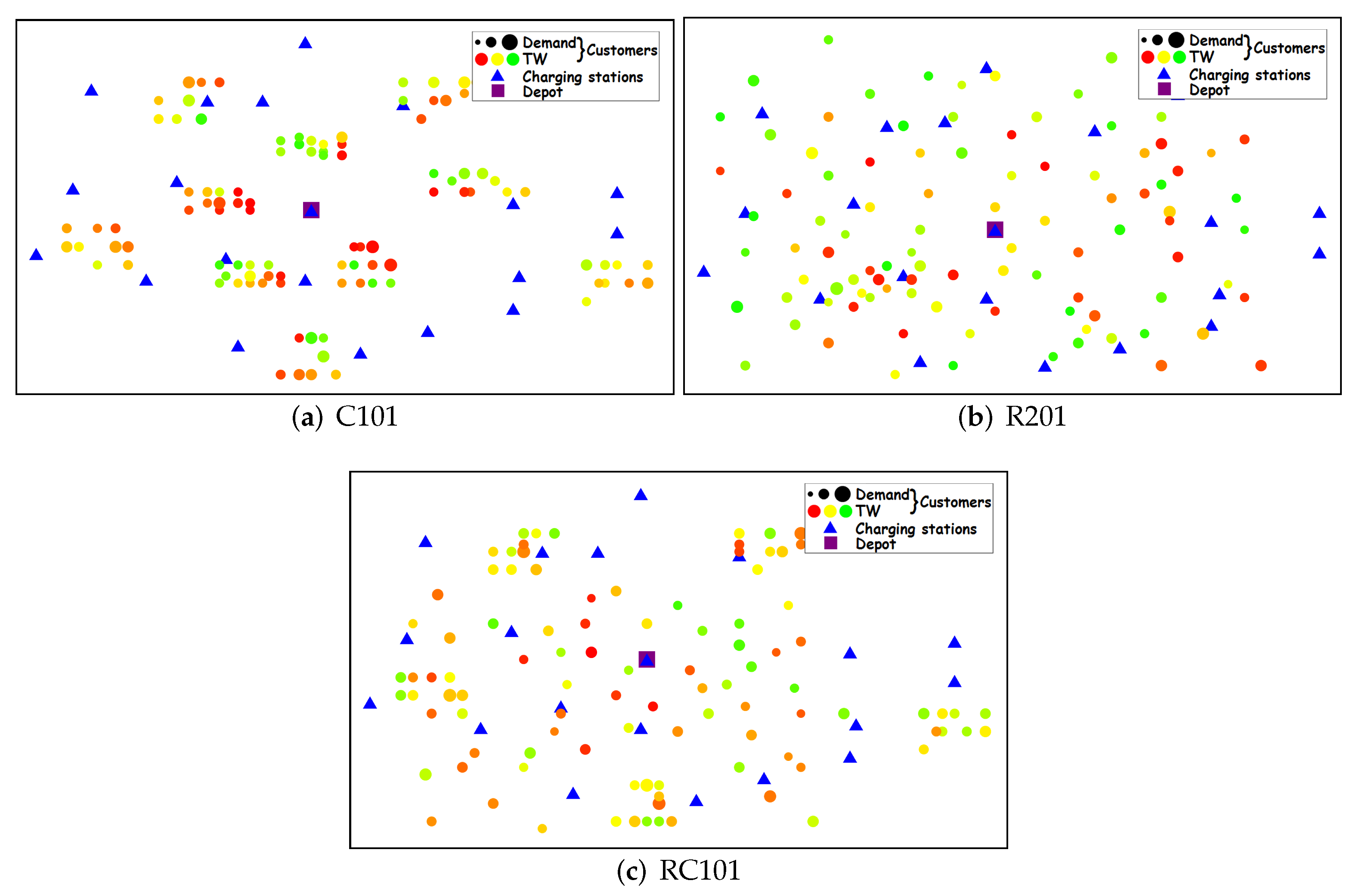
The materials include EVRPTW benchmark instances which consist of: (i) 56 large instances, each with 100 customers and 21 CSs, and (ii) 36 small instances, with 5, 10, and 15 customers per instance. The example of three instances is presented in Figure 1, where each customer is presented as a filled circle with two attributes: (i) size, which represents the demand of a customer—the greater the demand, the larger the circle, and (ii) color, from red to green, with red representing customers that close sooner (need to be visited sooner) and green representing customers that close later. The depot is represented with the purple rectangle, while the CSs are represented with blue triangles. In all instances, the Euclidean distance is used for distance computation. Each customer in an instance is directly reachable from the depot regarding the time windows, while regarding the energy, at maximum, two CSs are needed to visit each customer. Depending on the geographical distribution of the customers, instances are divided into three groups: clustered customer distribution (C) (example in Figure 1a), random customer distribution (R) (example in Figure 1b), and a mixture of both (RC) (example in Figure 1c). Additionally, the instances are divided into two groups based on the scheduling horizon: short scheduling horizon with narrow time windows (1) (examples in Figure 1a,c), and long scheduling horizon with wide time windows (2) (example in Figure 1b). For example, in instance named R201, R stands for random customer distribution, 2 for wide time windows, and 01 represents the instance number.
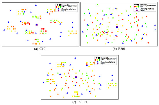
Figure 1.
Examples of EVRPTW instances.
Vehicle battery capacity Q, vehicle load capacity C, energy consumption rate r, and recharge rate g per instance group are presented in Table 1. It can be seen that instance groups with wider time windows have larger vehicle load and battery capacities, which consequently results in a lower number of vehicles per instance.

Table 1.
EVRPTW instances—group values.
3. Methodology
In this section, the ALNS metaheuristic is coupled with an exact procedure to solve the EVRPTW problems. Most of the algorithm framework is adopted from Schiffer and Walther [21] for the ELRPTW-PR and given by Algorithm 1. The basic idea of the method is to allow for searching in the infeasible search space. Therefore, the secondary objective function for solution s is given by Equation (17), as the sum of vehicle costs and penalties. represents the total cost of the vehicle v; , , and represent penalty (violation) values, respectively, load capacity, time windows, and battery capacity; and , and represent penalty coefficients [1,21].
Due to the infeasible search strategy, three solution instances were tracked during the search: (i) Temporal solution that stores good solution found in previous iterations (can be infeasible), (ii) the best solution that stores the best solution so far (can be infeasible), and (iii) the best feasible solution so far. In each iteration, the current solution s is destroyed and repaired with selected operators. If the cost function of a new solution s is within percentage of the , the LS procedure is performed. Additionally, if the cost function of new solution s after the LS procedure is within an percentage of the , the exact procedure that determines optimal CS positions is performed. Afterwards, an update of the solution instances occurs: (i) if a new solution s is better than the current temporal solution , s is set as ; (ii) if a new solution s is better than the best solution , s is set as ; (iii) if a new solution s is feasible and better than the best feasible solution so far , s is set as . During the search, several criteria were checked: (i) The criterion for the application of the route removal algorithm (line 4) (not used in the original ALNS for ELRPTW-PR [21]), (ii) criterion for the update of values related to the used destroy-and-repair operators (line 24), (iii) criterion for the update of penalty coefficients (line 27), and (iv) overall method finish criterion (line 3). All criteria are expressed as the reached number of iterations. To intensify the search, LS and exact procedure are used, while to diversify the search, the destroy-repair strategy is used. The scoring and selection mechanisms for destroy-and-repair operators are adapted from Keskin et al. [20]. The control of intensification and diversification phases is done by the adaptive update of penalty coefficients: multiplied by if in the last iterations, a penalty in best solution occurred, or divided by if in the last iterations, a penalty in the best solution did not occur.
| Algorithm 1 Adaptive large neighborhood search method. |
|
3.1. Initial Solution
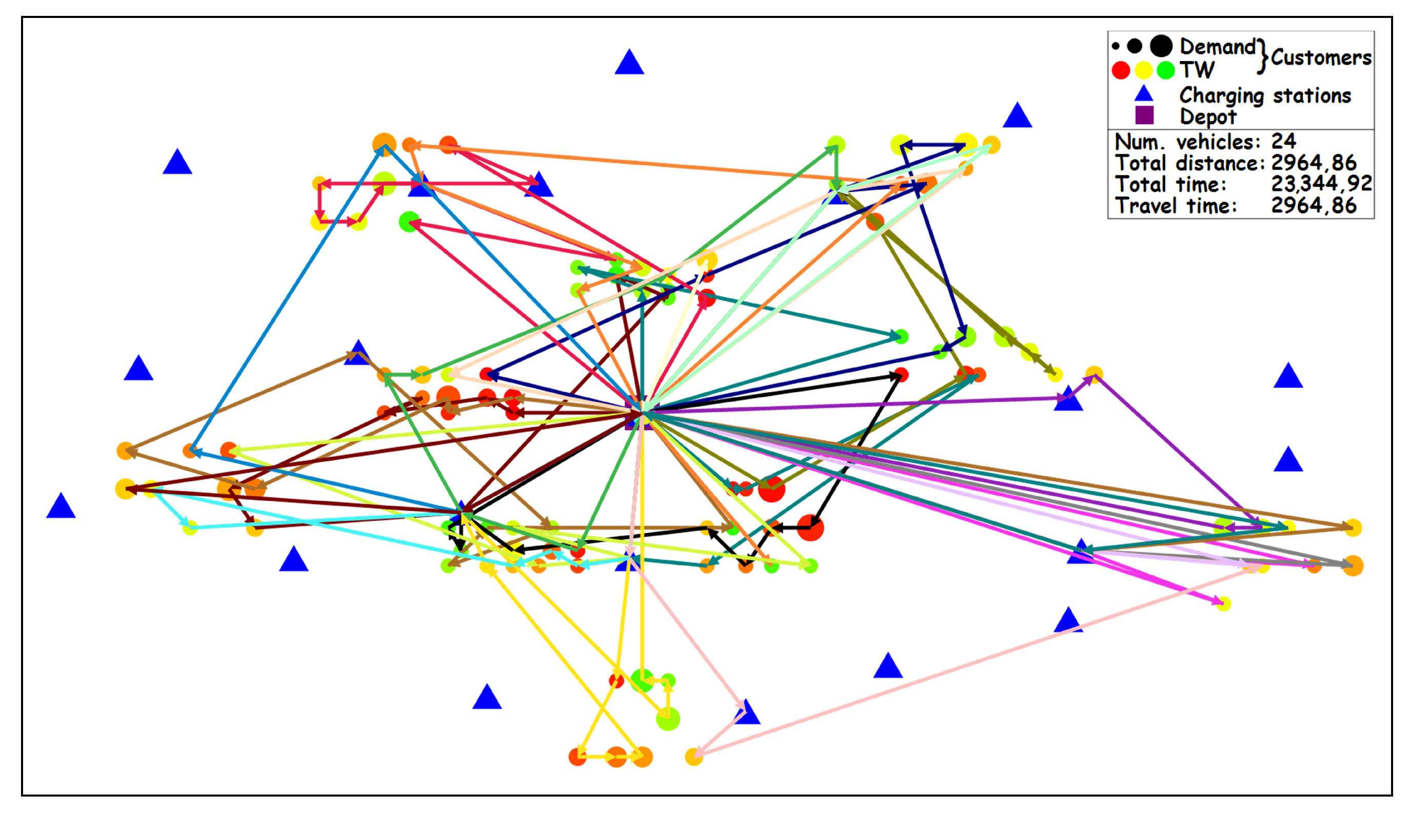
The initial solution is constructed by a new Greedy Time-Oriented Nearest Neighbor Heuristic (GTONNH) given by Algorithm 2. Vehicle routes are constructed in a serial way by adding customers, one by one, that satisfy all problem constraints: vehicle load capacity, customer time window, depot time window, and vehicle battery capacity. If none of the unserved customers could be added to the current vehicle route, the current vehicle route is closed, added to the solution s, and a new vehicle route is opened. The proposed procedure is based on the procedure of Felipe et al. [23], but it has two different parts. First, instead of adding the nearest CS when a vehicle cannot visit a customer due to the violation of battery capacity, a Multiple Best CS Insertion (MBCSI) procedure is performed to insert multiple CSs in the route to make it completely feasible (including the last visit to the depot). The MBCSI is based on the Best Station Insertion (BSI) method [20] with a FR strategy at each CS, but it additionally takes multiple CSs insertions into account to make the solution completely feasible. Second, in each iteration, the best customer with possible CS insertions (move M) is determined. The cost of a move is computed by Equation (18) [40], which takes into account an insertion distance increase (), total time increase , and spare time (time between the arrival time at customer and late time window) with , and coefficients controlling the ratios between them. The result of the GTONNH heuristic is, if possible, is a completely feasible EVRPTW-FR solution.
The example of the initial solution on instance C101 produced by GTONNH is presented in Figure 2. Each vehicle route is represented with different line colors. In total, 24 vehicles were produced, with a total traveled distance of .
| Algorithm 2 Greedy time-oriented nearest neighbor heuristic. |
|
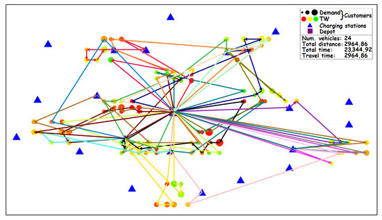
Figure 2.
GTONNH—Initial solution on instance C101.
3.2. Penalty Functions
As already mentioned, the penalties of the solution s are computed as the sum of penalties per each vehicle v in the solution s. Changes (moves) in the solution are frequently performed during the LS and destroy-repair phases, that is, to remove one customer from one place in the solution to another. The evaluation of these changes should be as fast as possible. The strategy of using concatenation operators for evaluation [41] is based on the principle that any route can be represented as the sum of its partial routes, meaning that a new route can be evaluated as the sum of two partial routes and a change of a customer schedule between them.
The load penalty is the easiest to compute, as it does not depend on the start time or the charging amount. If a vehicle route v is represented as a sequence of users , the vehicle load penalty can be computed by Equation (19) as the amount of total vehicle overload. The evaluation of load penalty between partial routes and can be done in for most of the basic move operators [42], given by the Equation (20). This requires tracking two forward variables for each user in route: rest load capacity (without over-penalization) and load violation .
In this paper, concatenation operators and variables regarding time windows and battery capacity are presented for EVRPTW-FR and EVRPTW-PR, based on the ones for ELRPTW-PR [21]. As EVRPTW-PR can be considered as a special case of the ELRPTW-PR, only small changes in the variables for EVRPTW-PR were needed, that is, that do not consider charging while serving the customer, while for EVRPTW-FR, new forward variables were proposed. Additionally, variables to determine charging schedules in both variants were added. As the proposed original approach is complex and hard to follow, in this paper, an additional description is given to ease the understanding.
3.2.1. EVRPTW-PR
The first important aspect of the approach presented by Schiffer and Walther [21] is to express all variables in the unit of time [22]. The energy consumed on a path is expressed as time needed to recharge the consumed energy. The battery capacity Q is also expressed as the time needed to fully charge the battery. The second important aspect is the so-called shifting rules [37]—traveling back in time to the latest feasible point in time when a violation occurs. This helps to not over-penalize violations. The description of forward variables is given in Table 2 with corresponding expression given by Equations (21)–(27).
Table 2.
Forward variables—EVRPTW-PR.
First of all, variables are propagated in forward fashion from the first depot in route to the last depot in route, that is, from user i to user j. The two basic variables are tracked: and , representing the earliest start time at user j by charging the minimum and maximum amount at preceding CSs. The shifted variants used to not over-penalize violations are expressed as and . The goal is to, whenever possible, use slack (spare) time for charging at previous CS. The spare time occurs when the vehicle arrives at a customer before the early time window and has to wait. The represents the time needed to charge the battery to the fullest with the assumption that minimum charging and spare charging was already performed. Sometimes, the whole amount of the spare time cannot be used for charging, because it would mean charging over the battery capacity Q. Therefore, the spare time is limited by the difference in time between charging minimum and maximum . The next important variable is the minimum charging time that has to be added at previous CS to be able to reach user j without the battery capacity (fuel) violation. This is perhaps the most important variable that allows the evaluation of basic moves in . If all spare times are used for recharging, then the additional charging that needs to be performed will linearly increase the start time at user j. Of course, if this additional amount exceeds the vehicle battery capacity Q at some point, the violation will be accounted for, but still, the start time at the user will need to increase by the corresponding additional recharging time.
The variable represents the minimum additional amount that has to be added at previous CSs, but it does not determine the charging amount at each CS. If the partial route up to j is feasible, this means that multiple feasible CS schedules can possibly be determined, which would produce the same arrival time at user j. To know the exact charging amount, at each CS, the original approach is improved with variables that track the charging amount at CSs, given by Equations (28)–(32). The charging time at CS is computed as the sum of spare time and additional charging time . By storing these values in the latest CS before user j, , as slack charging time and additional charging time , the exact charging schedule can be determined. Consequently, the cumulative charging in CSs and the cumulative recharging time corresponding to the used fuel amount (energy consumed) can also be computed. In some cases, where large spare times occur as vehicles have to wait for the start of the service, the vehicle could charge more than what is needed for traversing the route with the smallest charging amount possible. This occurs when condition is satisfied, as the sum of the full battery capacity and recharge amount at CSs is larger than the charging amount needed for traversing the route. On such occasions, if needed, a post-optimization procedure could be applied to determine a different charging schedule that decreases the charging amount at CSs.
The computation of forward time window violation is given by Equation (33), as the amount of time after the late time window. The computation of fuel violation is given by Equation (34) as the difference between and . The violation occurs when the sum of additional charging time added to the latest CS in route is greater than the maximum possible charging time at the latest CS.
Initial values of all forward variables at the depot are set to 0, .
To have an efficient move evaluation, beside the forward variables, the backward variables and penalties also have to be determined. The backward variables are presented in the Appendix A. The minimum functions are replaced by maximum functions, and is swapped by . The main idea is to propagate variables backwards, from the last depot in route to the first depot in route, that is, from user j to user i.
Concatenation operators for EVRPTW-PR are given by Equations (35)–(37). As these operators are not adequately described in the original paper, here, a more detailed explanation is given. For the concatenation of two partial routes and , first, the forward variables are propagated to user y, based on the forward variables of user x. Then, the time window of concatenated routes is computed by Equation (35) as the sum of forward time window violation of partial route , backward time window violation of partial route , and an additional two parts, noted with brackets (1) and (2). The first bracket (1) in Equation (35) represents the forward time window violation at user y consisting of the time window violation due to the late arrival at user y (bracket in Equation (35)) reduced by the over-penalization value equal to the forward fuel penalty at user y (bracket in Equation (35)). The second bracket (2) in Equation (35) represents the violation of the latest arrival time at user y, computed as the difference between the earliest feasible begin time (bracket in Equation (35)) and the latest arrival time with minimum charging amount , further reduced by the over-penalization value equal to the backward fuel penalty at user y (bracket in Equation (35)). As it can be seen, the general idea is to compute the time window violation in a typical way but to reduce it by both forward and backward fuel violations, to reduce the time window over-penalization.
The fuel violation is computed by Equation (36) as the sum of forward fuel violation of route , backward fuel violation of route , forward fuel violation at user y and additional value representing a case when the total route energy exceeds overall battery capacity. The value in bracket (3) in Equation (36) represents the additional charging time at user y if maximum charging is performed in both forward and backward directions. The value of D helps to reduce the over-penalization and differs depending on whether the user y is a CS, or not. In case the user y is not a CS, the overall difference is further reduced by possible spare charging time (bracket 4 in Equation (37)) at user y. The spare time for charging is computed as the sum of the time between and and the time between and (bracket in Equation (37)), and limited by the total spare time between the latest minimum start time and the earliest minimum start time at user y (bracket in Equation (37)). The computed spare time cannot be larger than H if user y is not a CS. If user y is a CS, then the spare time (bracket 5 in Equation (37)) that can be used for charging cannot be larger than the maximum charging time or the time violation between minimum forward and backward charging (bracket 6 in Equation (37)). The spare value (bracket 5 in Equation (37)) is computed as spare time between and reduced by the time window violation between maximum forward and backward charging .
Although not discussed by Schiffer and Walther [21], it is important to note that the used procedure does not compute an exact value of the violation, but rather it approximates the sum of the time window and fuel violations. The approximated fuel and time window values can differ significantly from the corresponding exact values, but their sum is close to the exact value. The reason is that it is hard to distinguish whether the time window violation is caused by the travel time or too much charging at CS. The important part of the procedure is that it never underestimates evaluation, especially for feasible moves.
3.2.2. EVRPTW-FR
For EVRPTW-FR, a similar approach as in EVRPTW-PR is applied. All the variable names are similar to the ones for the EVRPTW-PR, but instead of PR, the FR at each CS is considered, that is, the whole value of is used. The new forward variables are computed by Equations (38)–(42). The variable accounts for the additional recharging time, which here directly corresponds to the fuel violation. The slack times are always zero, as there is no spare time to charge the vehicle any further. The forward shifted variables, time window penalties and fuel penalties remain the same as in EVRPTW-PR, as well as all backward variables and penalties. The backward variables remain the same because the solution to the FR strategy in the second partial route , is somewhere in between, the backward latest minimum and maximum arrival time , depending on the charging amount in the forward direction. The time window concatenation operator remains the same, while the fuel concatenation operator is given by the Equation (43) without the value of D that helps to reduce the over-penalization in the PR variant. These equations represent the idea of concatenating two partial routes, the first one with the forward FR strategy and the second one with the backward PR strategy.
As in EVRPTW-FR, the latest start time for FR strategy is somewhere in between , the approximated violation can significantly differ from the exact one, but it still gives a good representation value to differ bad from good moves. Therefore, in this paper, we use a restricted move list that stores best moves during the search phase of each LS operator. At the end of each LS operator, moves are evaluated exactly with complexity, and the best one is selected.
3.3. Destroy-and-Repair Operators
The used destroy operators are the following: Worst removal [34], Related removal [43], Shaw removal [44], and CS vicinity [17]. The Related removal and Shaw removal operators consider removing customers that are close in some sense, while the Worst removal operator removes customers that incur the highest costs. CS vicinity operator removes a CS and all customers in a defined radial vicinity form it. The number of removed customers is selected at random in the interval, where is the number of customers in instance, and and are threshold percentage values. For the repair of the solution the Last-In First-Out (LIFO) strategy is used, meaning that the customers are inserted back in the solution based on their removal order [18,21]. In each iteration, four insertions are evaluated: (i) customer-only insertion; (ii) customer with preceding CS; (iii) customer with succeeding CS; and (iv) customer with both preceding and succeeding CS.
Additionally, a route removal algorithm is applied at certain points during the search. The algorithm removes one route at random and applies a similar ALNS framework as in Algorithm 1 to find a solution with a lower number of vehicles. The criteria for route removal tends to apply the route removal procedure more frequently at the beginning of the search and then gradually reduce its calls towards the end of the search.
3.4. Local Search and Optimal CS Placement
To improve the solution generated by destroy-and-repair operators, the following local search operators are used: Intra relocate, Intra exchange, Or-opt, Intra station in, Intra station out, Inter relocate, Inter exchange, Inter cross exchange (), and Inter 2-Opt* [7,45,46,47,48].
As CS configuration significantly influences the solution quality, after the local search, sometimes the optimal CS placement is performed. The applied algorithm is based on the forward labeling algorithms for the elementary shortest path problem with resource constraints for both the FR and PR strategy [22]. The used variables and equations are presented by Desaulniers et al. [22]. The basic idea is to remove CS visits in the route and then generate a limited search tree by extending the fixed route with CSs (paths). To reduce the search space, the dominance rules are applied between paths to discard paths that are always worse than other paths (dominated by other paths). For the evaluation of paths and dominance comparison, the labeling technique is used.
3.5. Example of a Search Process
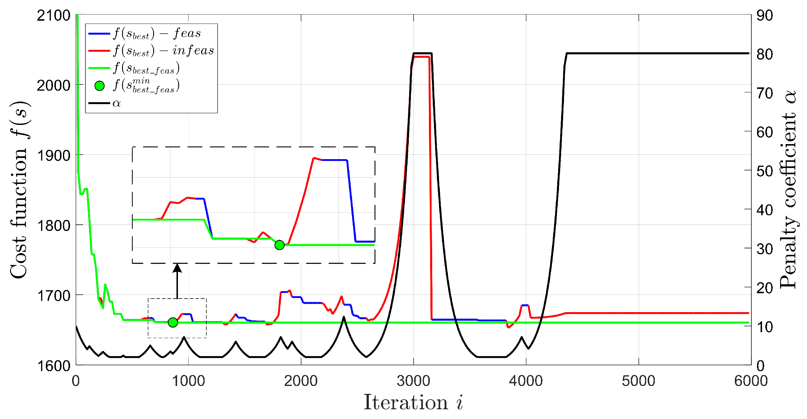
The example of a cost function during the search process when solving EVRPTW-FR on instance R101 is presented in Figure 3. The values of penalty coefficient are plotted with black color and presented on the right y axis. On the left y axis are the values of the cost function for the best solution (blue line for the feasible part and red line for the infeasible part), and best feasible solution (green line). The first occurrence of the best overall feasible solution is represented with a green circle. The update value of penalties is , and the penalties are updated every iterations. The cost value of the initial solution is . It can be seen that the feasible solution is rapidly improved at the beginning of the search, with occasional spikes. These spikes represent that the feasible solution with a lower number of vehicles is found and that it is accepted although it has a worse cost function value. When the best solution is infeasible but accepted due to the acceptance criteria (red lines), the penalty coefficient increases, while the opposite occurs when the best solution is feasible. In the zoomed part, it can be seen that allowing infeasible solutions can lead to better feasible solutions. Additionally, as the minimum best feasible solution is relatively quickly found (), in the rest of the search, the infeasible solutions are accepted, and penalties are updated to perhaps find a better solution.
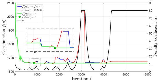
Figure 3.
Cost function in search process—R101—EVRPTW-FR.
The example of applied destroy-and-repair operators on instance C101, together with the example of operators selection probabilities are presented in Appendix B.
4. Results
In this section, the proposed ALNS method is run on benchmark EVRPTW instances and compared to the BKSs from the literature. The ALNS is implemented as a single-thread code in the C# programming language. All tests were performed on a machine with an Intel E5 processor and 32 GB of RAM. The floating-point precision used for the comparison was set to . Most of the ALNS parameters are similar to the one of Schiffer and Walther [21], except the following: (i) coefficients controlling ratios in GTONNH—, , , (ii) total number of iterations 10,000, (iii) number of restricted LS moves , and (iv) lower and upper percentage threshold for the number of customers removed . The text files containing results of ALNS on benchmark EVRPTW instances are available https://www.fpz.unizg.hr/zits/?page_id=1424 (accessed on 9 December 2021).
4.1. EVRPTW-PR
The results of distance minimization in EVRPTW-PR are presented in Table 3. The ALNS was run 10 times on each instance. The results are compared to the BKSs of Hierman et al. [19] (HIER), Keskin et al. [20] (KESK) and Schiffer and Walther [21] (SCHI). Here, we have to note that some BKSs reported by SCHI have a possibly wrong number of vehicles. The authors stated that they compared their results to the results of KESK [20] but did not use the BKS values presented in the paper; rather, they used some different reference values which are not available in the literature. Therefore, we tried to correct the number of vehicles reported by SCHI to make the comparison reliable. Further on, three columns are used to represent BKSs values: name N, vehicle number K, and total traveled distance d. For the ALNS, the following columns are presented: average vehicle number , best vehicle number , the difference in best vehicle number between BKS and ALNS, average total traveled distance , best total traveled distance , total traveled distance relative difference and percentage relative difference between BKS and ALNS, total time of the best solution , recharging amount of the best solution , number of CSs in the best solution m, and average execution time in minutes. The relative percentage difference was computed as . It is important to note that in relative distance computation, and , only the solutions in which the ALNS produced the minimum number of vehicles were considered, because otherwise, with a higher number of vehicles, the total traveled distance decreases which then produces a wrong comparison. Lastly, the initial solution values produced by GTONNH are presented in the last two columns: initial vehicle number , and initial total traveled distance . The summary of the results is presented in the last two rows as averaged and summed values. All rows in which the ALNS produced a better solution regarding the vehicle number or the total traveled distance are bolded.
Table 3.
EVRPTW-PR distance—results.
In 29 out of 56 instances, the ALNS found a better solution, with in total 9 vehicle less, and average relative percentage difference in the total traveled distance, meaning that even if the lower number of vehicles is found, the ALNS finds a good user configuration in terms of distance minimization. The average value of the average vehicle number has a lower value than the average of the BKSs vehicle number, indicating the good average performance of the ALNS. The sum of the total time in all instances consists of: travel time—%, service time—%, waiting times—% and charging time—%. As it can be seen, most of the total time is spent on service, while the least time is spent on charging and waiting. On average, 10 CSs are visited per instance and per vehicle route. Additionally, on average, vehicle leaves the CS with the rest battery capacity equal to % of full battery capacity. In terms of an average execution time, the ALNS execution time of min is comparable to HIER ( min) and KESK ( min), but worse than SCHI ( min).
As expected, GTONNH produced feasible initial solutions that are far from the best ones, as an initial feasible solution is hard to achieve. In the total sum of vehicle number, GTONNH produced % vehicle more, with also an increase in the total traveled distance by %.
The results also differ depending on the instance group. It can be seen that on instance groups with shorter time windows (, and ), which also have a lower battery capacity Q, a larger number of vehicles is produced. The , and especially R instances, are harder to solve than C instances due to the larger feasible solution space. This is especially the case in and instance groups, where the execution time significantly increases due to the larger number of customers per route and frequent application of LS and exact CS placement procedure.
To see the influence of integrating BEVs in the goods delivery, the results are compared to the BKSs on Solomon VRPTW instances, downloaded from https://www.sintef.no/projectweb/top/vrptw/solomon-benchmark/ page (accessed on 9 December 2021). In total, the BKSs on VRPTW instances contain 405 vehicles and produce the total traveled distance of 57,186.88. Although the direct comparison is not entirely correct as some customers in VRPTW instances have relaxed time windows in EVRPTW instances [1], still some general conclusion could be drawn, that even with the relaxed time windows, the EVRPTW-PR produced % more vehicles and increased total traveled distance by %.
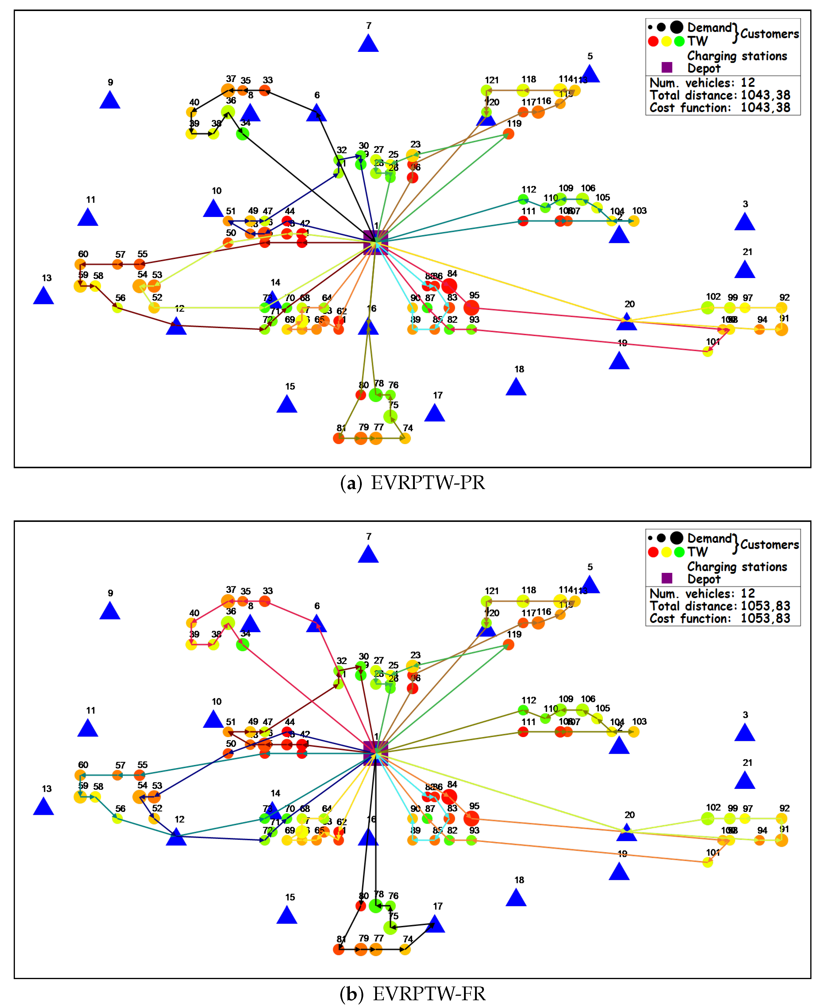
The example of BKS on EVRPTW-PR C101 instance is presented in Figure 4a. In total, 12 vehicles are presented, each with different color, with the total traveled distance of . To compare the recharge strategies, additionally user IDs are added above circles in the Figure 4.
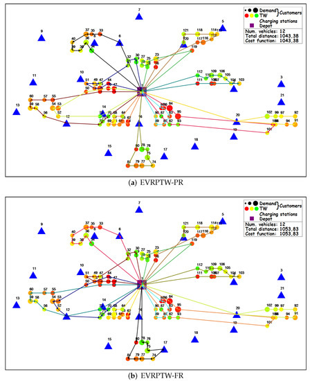
Figure 4.
C101: BKSs.
4.2. EVRPTW-FR
The results of distance minimization in EVRPTW-FR are presented in Table 4. The ALNS was again run 10 times, and the same columns as in the EVRPTW-PR variant are used, except the columns for GTONNH, as it has the same values per instance as in the PR variant. The results are compared to the BKSs of: Schneider et al. [1] (SCHN), Goeke et al. [17] (GOEK), Hierman et al. [18] (HIE1), Hierman et al. [19] (HIE2), Keskin et al. [20] (KESK) and Schiffer et al. [21] (SCHI). It can be seen that ALNS was not able to reduce the number of vehicles on four instances: , , and . Nevertheless, nine new BKSs (bold font) are found for instances: , , , , , , , and . The total traveled distance is lower than in BKSs, due to the higher number of vehicles.
Table 4.
EVRPTW-FR distance—results.
Compared to the FR strategy, it can be seen that PR strategy produced 18 vehicles less, with also decrease in the sum of the total traveled distance (%) and the sum of the total time (%). As a result, a PR strategy uses 48 CSs more, but actually charges less, as a recharge amount is % lower than the one for the FR. The total time in all instances consists of the following percentages: travel time—%, service time—%, waiting times—% and charging time—%. Here again, it can be seen that the charging time with the FR strategy is greater than the charging time with the PR strategy. The average execution time for FR strategy is min. The produced time is slightly higher than the one in the PR strategy due to the additional evaluation of best moves exactly in the LS. Compared to the BKSs of VRPTW instances, the ALNS in EVRPTW-FR produced 39 vehicles more (%) and increased total traveled distance by %.
The example of BKS on EVRPTW-FR C101 instance is presented in Figure 4b, with in total 12 vehicles and total traveled distance of .
To show the difference between the FR and PR strategies, one route is selected for the comparison. It is important to note, that the optimization procedure in most of the cases produces different customer and CS schedules for routes in different EVRPTW variants, which makes the direct comparison between routes non applicable. But here, there are some routes that have similar customer schedule but differ in CS schedule. This happened as routes with FR and PR strategies on clustered instances overlap in grater extent than, for example, routes on random instances. The comparison is conducted for route 1—dark green route in EVRPTW-PR (Figure 4a) and black route in EVRPTW-FR (Figure 4b). The following rows are presented in Table 5 and Table 6: user ID (ID), time window (TW), service time (ST), remaining load capacity (RL), arrival distance (AD), arrival time (AT), start time of service (BT), remaining battery capacity (RB), charging time (CT) and recharged capacity (RC). Color of the user’s ID matches the color of the user’s circle in Figure 4. It can be seen that the PR strategy has two visits to the CS 16, while the FR strategy has only one visit to CS 17. The fuel and time related variables differ between the variants, while the remaining load capacity variable has the same values. The arrival distance at the depot (vehicle total traveled distance) is lower for PR than for the FR strategy, as well as the total recharge amount (). Although less time is spent on charging, the arrival time at the depot (vehicle total time) is actually higher for the PR strategy than the FR strategy. Usually, this is not the case, but here it happened as vehicle visits a CS immediately before the depot. To further show the difference PR and FR strategies, the route with the PR strategy is evaluated as a route with a FR strategy. The rows are presented at the end of the Table 6. It can be seen that there is no change at the first CS, as the vehicle is recharged to full capacity in both strategies. The only difference is in the second visited CS, where in the PR strategy, the vehicle is recharged by only a small amount needed to finish the route, while in the FR strategy, the vehicle is recharged to the fullest (% of the full battery capacity), resulting in an infeasible arrival time at the depot (violation of the depot late time window). The evaluation of a route with a FR strategy as a route with PR strategy would produce the same solution as the FR strategy, as the almost whole spare time at CS 17 () can be used for charging to the fullest.
Table 5.
Values in route 1—FR.
Table 6.
Values in route 1—PR.
4.3. Evaluation Test
As already highlighted, the evaluation of a change in the route with FR and PR strategy can be done in for most of the basic operators, but FR requires additional exact evaluation. As in the original research for ELRPTW-PR, the difference between exact and approximated violation values was not reported; here, a small test was conducted.
To validate the evaluation variables and operators, the testing was performed on instance [20] with the total number of iterations set to . The results are presented in Table 7 as a difference between approximated evaluation and exact evaluation. The positive values represent an overestimation of penalties, while the negative values represent underestimation. Column Feas/Infeas represents either a completely feasible move or an infeasible move (evaluated exactly). It can be seen that operators for the PR strategy never underestimate violations as column Min in Total is zero in all cases. Although the time window and fuel by itself can be underestimated, their sum is not, meaning that the underestimation of time windows is compensated with fuel violation. On average, the penalty violations are overestimated by the value of , even for the completely feasible moves where the value is .
Table 7.
Evaluation.
For the FR strategy, the mean total violations are even lower than in PR strategy, with the value of . For completely feasible moves, there was not an underestimation of total violation, and the mean value of violation is . As it can be seen, in the FR strategy, the underestimation of total violations occur up to , and also the overestimation values are greater, almost doubled compared to the PR strategy. This is the main reason why the latter exact evaluation of the best moves was used in the LS procedure. Interestingly, the fuel violation is never underestimated.
5. Discussion
The selection of the recharging strategy depends on the delivery problem characteristics and decision-makers. In the following paragraphs, the results of the paper regarding the used recharging strategy are summarized.
- With the PR strategy, greater savings can be achieved, but in real-life application, it is harder to implement as drivers need to visit CSs more frequently and perform time-precise charging with a high possibility of leaving a CS without a fully charged battery.
- Maintaining the energy reserve in the PR strategy to overcome the so-called range anxiety [15,49]—a fear that the vehicle range will not be enough to complete the designated route. The reason is that the amount of the energy recharged at the CS is usually only enough to reach the next CS or depot, which is not flexible enough for the application in real-life where the travel time is time-dependent [50], as well as waiting times that can occur at CSs which prolong delivery time [30].
- On the other hand, significant savings can be achieved by the PR strategy, as the total number of vehicles decreased by % and the total traveled distance decreased by compared to the FR strategy. Additional savings could also be achieved by PR strategy as the amount of energy recharged during the day at public or private CSs is almost 30% less than the amount of energy recharged with the FR strategy. In the PR strategy, the minimal amount of energy could be recharged during the day when electricity costs are higher, and the rest of the energy could be recharged during the night.
- The PR strategy also helps to reduce the battery degradation and to prolong the battery life [51] as it escapes charging at a CSs with high SoC values (in numerical tests, it was shown that on average, the vehicle leaves a CS with the SoC value of %. Additionally, if a more realistic non-linear charging process that prolongs charging time after approx. 80% of the SoC value is considered [25], the FR strategy would lead to a higher number of infeasible solutions than the PR strategy.
- Comparison between BKSs on VRPTW instances and the best ALNS solutions for FR and PR variants indicates that integration of BEVs in the delivery processes increases the total vehicle number by at least % and the total traveled distance by at least %. Additional analysis should be conducted to validate if the reduction of transportation costs by BEVs can compensate for the increase in the vehicle number and total traveled distance.
There are several research directions left for future research. First, the evaluation of moves in the EVRPTW-FR could perhaps be done in without the need for additional evaluation, by the use of a bidirectional exact procedure [22]. The second direction is the extension of the proposed methodology on the EVRPTW problem with different charger types at CSs [16]. The third direction is the consideration of dynamic traffic conditions on the road network in terms of the time-dependent travel time [52], as well as different secondary objectives: total time, travel time, recharging costs, recharging amount, and so forth.
6. Conclusions
In this paper, the delivery of goods with electric vehicles was observed through the solution of the EVRPTW problem, which aims to determine the minimum number of vehicles and the minimum total distance traveled needed to perform the delivery. Two recharging strategies were considered: FR and PR. For the creation of the initial solution, a new GTONNH heuristic is proposed, which produces a feasible solution with a relatively high number of vehicles due to the narrow feasible solution space. The route removal, local search and exact procedures were integrated within the ALNS framework to further intensify the search and lead to better solutions. The proposed ALNS metaheuristic uses the approximation of changes in the solution, which results in evaluation of moves for the PR strategy. The FR strategy also uses evaluation of moves, but additional exact evaluation is performed on best moves.
On 56 benchmark EVRPTW instances, the proposed ALNS metaheuristic was able to find 29 new BKSs for EVRPTW-PR and 9 BKSs for EVRPTW-FR. The PR strategy was able to reduce the total vehicle number, total distance traveled, total time and total recharging amount compared to the FR strategy, at the expense of the increase in the number visited CSs. The PR strategy turned out to be more robust regarding the battery degradation costs, non-linear charging function, and daily charging costs, but it has to have a high compliance rate to be efficient in the real-life application. Compared to the BKSs on VRPTW instances, which do not consider delivery with BEVs, the total number of vehicles increased by at least 5% in EVRPTW problems, and the additional cost-effectiveness of BEVs application for goods delivery should be investigated.
Author Contributions
Conceptualization, T.E. and T.C.; methodology, T.E.; software, T.E.; validation, T.E.; resources, T.C.; writing—original draft preparation, T.E.; writing—review and editing, T.E.; visualization, T.E.; supervision, T.C.; project administration, T.C.; funding acquisition, T.C. All authors have read and agreed to the published version of the manuscript.
Funding
This research was funded by the University of Zagreb, as a part of grants for basic financing of scientific and artistic activities in the academic year 2020/2021 within two projects: Innovative control strategies for sustainable mobility in smart cities and Optimization of the line transport timetables for the case of electric vehicles: a proof of concept. The APC was funded by the University of Zagreb, Faculty of Transport and Traffic Sciences. Additionally, the research has been partially supported by other two sources: Croatian Science Foundation under project IP-2018-01-8323 and project KK.01.1.1.01.0009 (DATACROSS) within the activities of the Centre of Research Excellence for Data Science and Cooperative Systems supported by the Ministry of Science and Education of the Republic of Croatia.
Institutional Review Board Statement
Not applicable.
Informed Consent Statement
Not applicable.
Data Availability Statement
EVRPTW benchmark instances: https://data.mendeley.com/datasets/h3mrm5dhxw/1 (accessed on 9 December 2021); EVRPTW-FR/PR BKSs values found by the proposed ALNS metaheuristic https://www.fpz.unizg.hr/zits/?page_id=1424 (accessed on 9 December 2021).
Conflicts of Interest
The authors declare no conflict of interest. The funders had no role in the design of the study; in the collection, analyses, or interpretation of data; in the writing of the manuscript, or in the decision to publish the results.
Abbreviations
The following abbreviations are used in this manuscript:
| BEV | Battery electric vehicle |
| BKS | Best known solution |
| BSI | Best station insertion |
| CS | Charging station |
| ELRPTW-PR | Electric location routing problem with time windows and partial recharging |
| EV | Electric vehicle |
| EVRP | Electric vehicle routing problem |
| EVRPTW | Electric vehicle routing problem with time windows |
| EVRPTW-FR | Electric vehicle routing problem with time windows and full recharge |
| EVRPTW-PR | Electric vehicle routing problem with time windows and partial recharge |
| FR | Full recharge |
| GHG | Greenhouse gas |
| GTONNH | Greedy time-oriented nearest neighbor heuristic |
| ICEV | Internal combustion engine vehicle |
| LIFO | Last-in first-out |
| LS | Local search |
| MBCSI | Multiple best charging station insertion |
| MILP | Mixed integer linear program |
| NP | Non-deterministic polynomial |
| PHEV | Plug-in hybrid electric vehicle |
| PR | Partial recharge |
| SoC | State of charge |
| VRP | Vehicle routing problem |
| VRPTW | Vehicle routing problem with time windows |
Appendix A
The used backward variables are presented in Table A1 and are computed by Equations (A1)–(A7). The backward time window and fuel violations are given by Equations (A8) and (A9). The initial values for backward variables related to the time of the last user in route are set to the late time window, , while the fuel related variable is set to zero, .
Table A1.
Backward variables—EVRPTW-PR.
Table A1.
Backward variables—EVRPTW-PR.
| Symbol | Description |
|---|---|
| Latest start time at user i with charging minimum amount as possible before i | |
| Latest start time at user i with charging maximum amount possible at preceding CSs with the assumption that minimum charging was performed before preceding CS | |
| Time needed to charge to maximum at user i with charging minimum amount as possible before i | |
| Slack time at user i | |
| Additional charging time at user i that has to be added at preceding CSs | |
| Shifted latest start time at user i when violation occurs with charging minimum amount as possible before i | |
| Shifted latest start time at user i when violation occurs with charging maximum amount possible at preceding CS with assumption that minimum charging was performed before preceding CS |
Appendix B
The selection probabilities of the operators change depending on their performance. The example of how probabilities change for used operators in EVRPTW-PR on instance C101 is presented in Figure A1. The update of operator probabilities occurs every iterations. As it can be seen, different operators are preferred in different stages of the search. The related and CS vicinity destroy operators show lower probabilities than worst and Shaw destroy operators. The probability of related operator increased in the last phase, showing its benefits in the cases when the search is near the best found local optima. The sequential insertion operator is preferred in the early stages of the search when more frequently, better solutions are found. But later on, when the search gets stuck in the local optima, the perturbed variant shows its benefits.
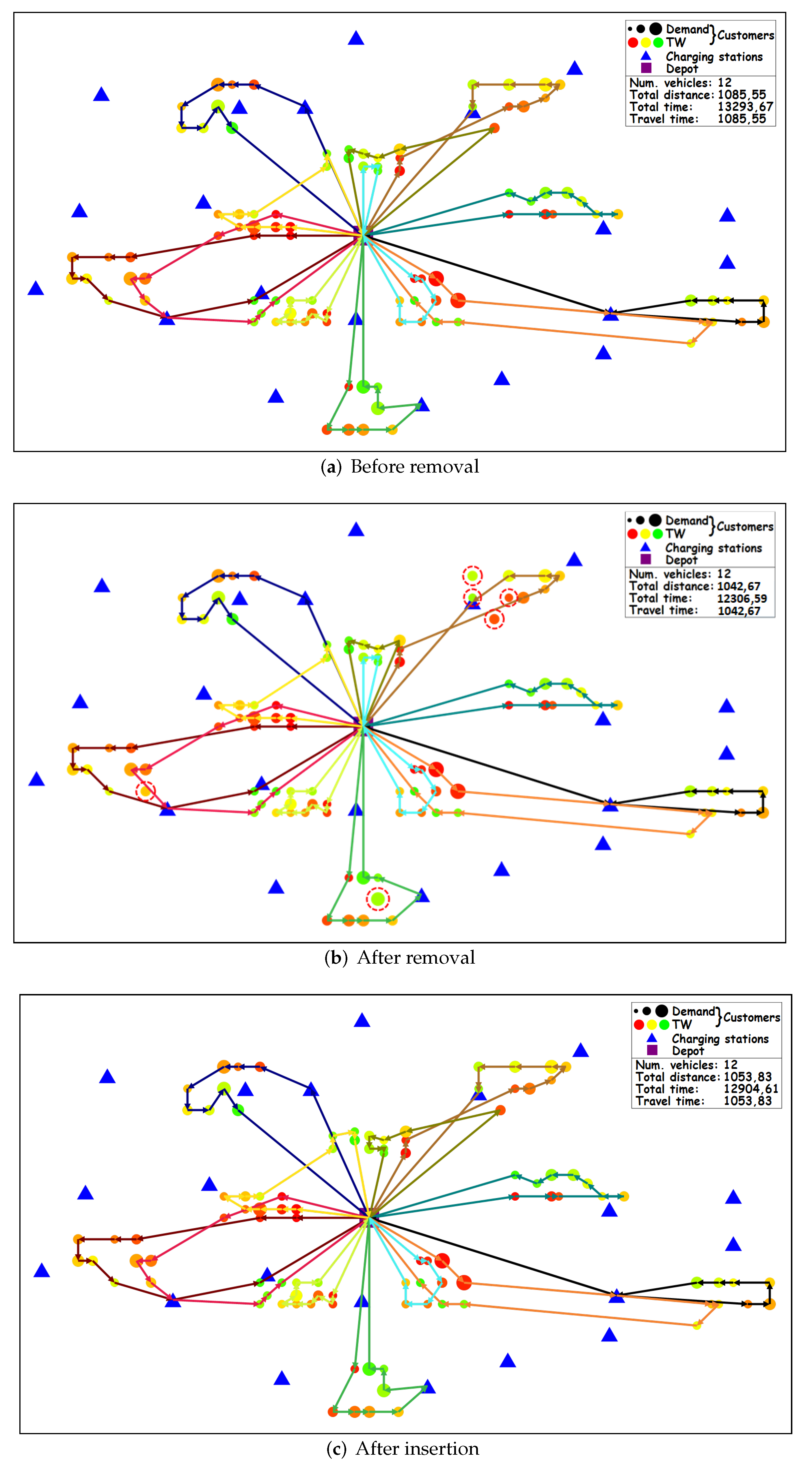
The example of the ALNS heuristic on the C101 instance and EVRPTW-FR problem is presented in Figure A2. The vehicle number remained the same, while the distance traveled decreased from before removal to after insertion. The removed customers are presented with red dashed circles.

Figure A1.
Example of operator probabilities: C101 -EVRPTW-PR.
Figure A1.
Example of operator probabilities: C101 -EVRPTW-PR.
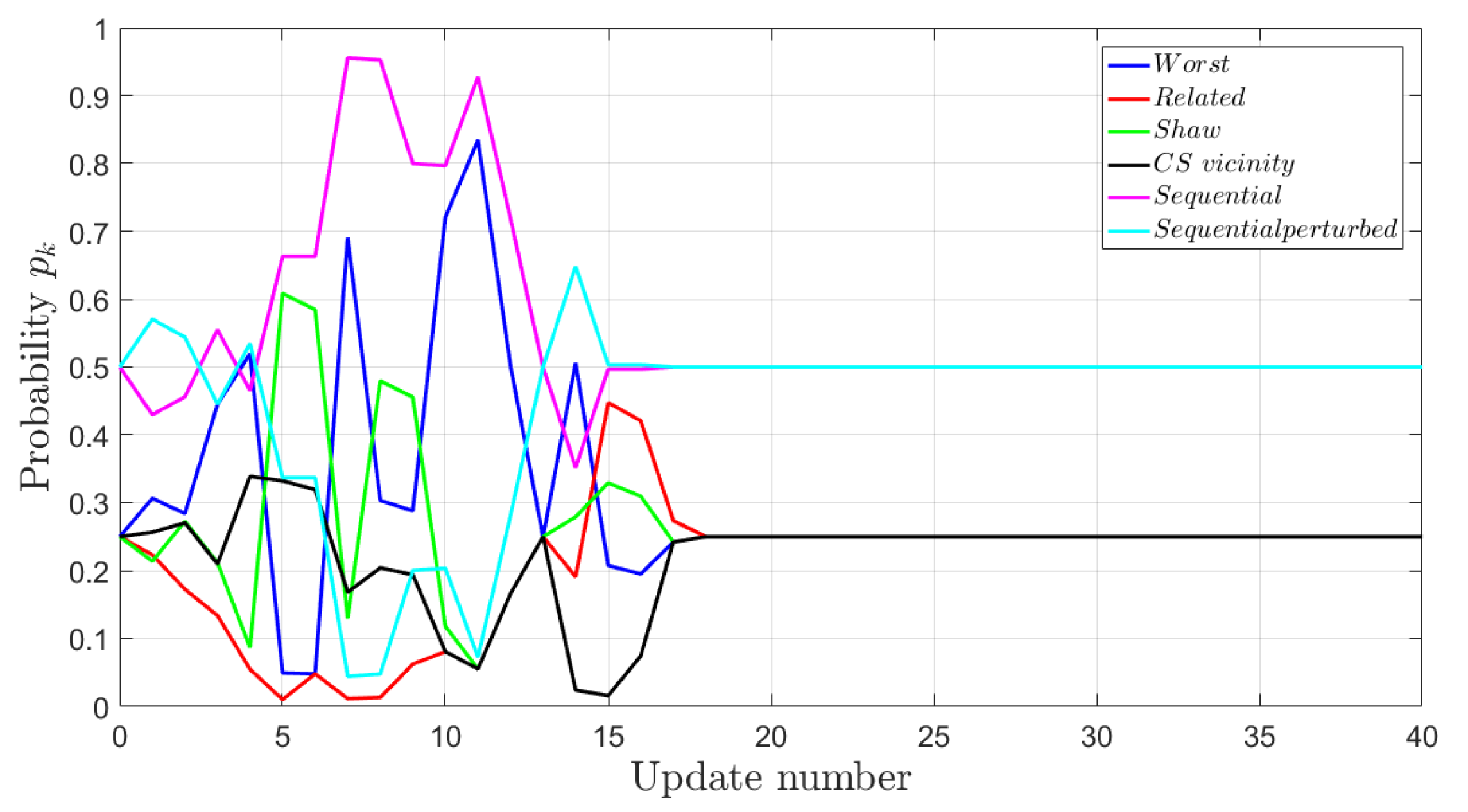
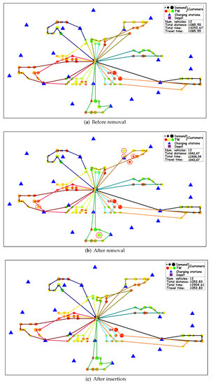
Figure A2.
ALNS example: C101—EVRPTW-FR.
Figure A2.
ALNS example: C101—EVRPTW-FR.
References
- Schneider, M.; Stenger, A.; Goeke, D. The Electric Vehicle-Routing Problem with Time Windows and Recharging Stations. Transp. Sci. 2014, 48, 500–520. [Google Scholar] [CrossRef] [Green Version]
- Vidal, T.; Crainic, T.G.; Gendreau, M.; Prins, C. Heuristics for multi-attribute vehicle routing problems: A survey and synthesis. Eur. J. Oper. Res. 2013, 231, 1–21. [Google Scholar] [CrossRef]
- Toth, P.; Vigo, D. (Eds.) The Vehicle Routing Problem; Society for Industrial and Applied Mathematics: Philadelphia, PA, USA, 2001. [Google Scholar]
- WEEA. Greenhouse Gas Data—Emissions Share by Sector in EU28. 2015. Available online: http://www.eea.europa.eu/data-and-maps/data/data-viewers/greenhouse-gases-viewer (accessed on 31 August 2020).
- European Commission. Effort Sharing: Member States’ Emission Targets. 2009. Available online: https://ec.europa.eu/clima/policies/effort_en (accessed on 7 February 2021).
- Davis, B.A.; Figliozzi, M.A. A methodology to evaluate the competitiveness of electric delivery trucks. Transp. Res. Part E Logist. Transp. Rev. 2013, 49, 8–23. [Google Scholar] [CrossRef]
- Erdelić, T.; Carić, T. A Survey on the Electric Vehicle Routing Problem: Variants and Solution Approaches. J. Adv. Transp. 2019, 2019, 1–48. [Google Scholar] [CrossRef]
- Moon, S.; Lee, D.J. An optimal electric vehicle investment model for consumers using total cost of ownership: A real option approach. Appl. Energy 2019, 253, 113494. [Google Scholar] [CrossRef]
- Feng, W.; Figliozzi, M. An economic and technological analysis of the key factors affecting the competitiveness of electric commercial vehicles: A case study from the USA market. Transp. Res. Part C Emerg. Technol. 2013, 26, 135–145. [Google Scholar] [CrossRef]
- Young, K.; Wang, C.; Wang, L.Y.; Strunz, K. Electric Vehicle Battery Technologies. In Electric Vehicle Integration into Modern Power Networks; Garcia-Valle, R., Peças Lopes, J.A., Eds.; Springer: New York, NY, USA, 2013; pp. 15–56. [Google Scholar] [CrossRef]
- Wróblewski, P.; Lewicki, W. A Method of Analyzing the Residual Values of Low-Emission Vehicles Based on a Selected Expert Method Taking into Account Stochastic Operational Parameters. Energies 2021, 14, 6859. [Google Scholar] [CrossRef]
- Hao, X.; Lin, Z.; Wang, H.; Ou, S.; Ouyang, M. Range cost-effectiveness of plug-in electric vehicle for heterogeneous consumers: An expanded total ownership cost approach. Appl. Energy 2020, 275, 115394. [Google Scholar] [CrossRef]
- Bräysy, O.; Gendreau, M. Vehicle Routing Problem with Time Windows, Part I: Route Construction and Local Search Algorithms. Transp. Sci. 2005, 39, 104–118. [Google Scholar] [CrossRef] [Green Version]
- Macrina, G.; Pugliese, L.D.P.; Guerriero, F.; Laporte, G. The green mixed fleet vehicle routing problem with partial battery recharging and time windows. Comput. Oper. Res. 2019, 101, 183–199. [Google Scholar] [CrossRef]
- Barco, J.; Guerra, A.; Muñoz, L.; Quijano, N. Optimal Routing and Scheduling of Charge for Electric Vehicles: Case Study. Math. Probl. Eng. 2013, 2017, 8509783. [Google Scholar] [CrossRef] [Green Version]
- Keskin, M.; Çatay, B. A matheuristic method for the electric vehicle routing problem with time windows and fast chargers. Comput. Oper. Res. 2018, 100, 172–188. [Google Scholar] [CrossRef]
- Goeke, D.; Schneider, M. Routing a mixed fleet of electric and conventional vehicles. Eur. J. Oper. Res. 2015, 245, 81–99. [Google Scholar] [CrossRef]
- Hiermann, G.; Puchinger, J.; Ropke, S.; Hartl, R.F. The Electric Fleet Size and Mix Vehicle Routing Problem with Time Windows and Recharging Stations. Eur. J. Oper. Res. 2016, 252, 995–1018. [Google Scholar] [CrossRef] [Green Version]
- Hiermann, G.; Hartl, R.F.; Puchinger, J.; Vidal, T. Routing a mix of conventional, plug-in hybrid, and electric vehicles. Eur. J. Oper. Res. 2019, 272, 235–248. [Google Scholar] [CrossRef] [Green Version]
- Keskin, M.; Çatay, B. Partial recharge strategies for the electric vehicle routing problem with time windows. Transp. Res. Part C Emerg. Technol. 2016, 65, 111–127. [Google Scholar] [CrossRef]
- Schiffer, M.; Walther, G. An Adaptive Large Neighborhood Search for the Location-routing Problem with Intra-route Facilities. Transp. Sci. 2018, 52, 331–352. [Google Scholar] [CrossRef]
- Desaulniers, G.; Errico, F.; Irnich, S.; Schneider, M. Exact Algorithms for Electric Vehicle-Routing Problems with Time Windows. Oper. Res. 2016, 64, 1388–1405. [Google Scholar] [CrossRef]
- Felipe, Á.; Ortuño, M.T.; Righini, G.; Tirado, G. A heuristic approach for the green vehicle routing problem with multiple technologies and partial recharges. Transp. Res. Part E Logist. Transp. Rev. 2014, 71, 111–128. [Google Scholar] [CrossRef]
- Masmoudi, M.A.; Hosny, M.; Demir, E.; Genikomsakis, K.N.; Cheikhrouhou, N. The dial-a-ride problem with electric vehicles and battery swapping stations. Transp. Res. Part E Logist. Transp. Rev. 2018, 118, 392–420. [Google Scholar] [CrossRef] [Green Version]
- Montoya, A.; Guéret, C.; Mendoza, J.E.; Villegas, J.G. The electric vehicle routing problem with nonlinear charging function. Transp. Res. Part B Methodol. 2017, 103, 87–110. [Google Scholar] [CrossRef] [Green Version]
- Froger, A.; Mendoza, J.E.; Jabali, O.; Laporte, G. Improved formulations and algorithmic components for the electric vehicle routing problem with nonlinear charging functions. Comput. Oper. Res. 2019, 104, 256–294. [Google Scholar] [CrossRef] [Green Version]
- Yang, J.; Sun, H. Battery swap station location-routing problem with capacitated electric vehicles. Comput. Oper. Res. 2015, 55, 217–232. [Google Scholar] [CrossRef]
- Hof, J.; Schneider, M.; Goeke, D. Solving the battery swap station location-routing problem with capacitated electric vehicles using an AVNS algorithm for vehicle-routing problems with intermediate stops. Transp. Res. Part B Methodol. 2017, 97, 102–112. [Google Scholar] [CrossRef]
- Schiffer, M.; Walther, G. The electric location routing problem with time windows and partial recharging. Eur. J. Oper. Res. 2017, 260, 995–1013. [Google Scholar] [CrossRef]
- Keskin, M.; Laporte, G.; Çatay, B. Electric Vehicle Routing Problem with Time-Dependent Waiting Times at Recharging Stations. Comput. Oper. Res. 2019, 107, 77–94. [Google Scholar] [CrossRef]
- Kullman, N.D.; Goodson, J.; Mendoza, J.E. Dynamic Electric Vehicle Routing: Heuristics and Dual Bounds; HAL. 2018. Working Paper or Preprint. Available online: https://hal.archives-ouvertes.fr/hal-01928730 (accessed on 20 December 2021).
- Schiffer, M.; Schneider, M.; Walther, G.; Laporte, G. Vehicle Routing and Location Routing with Intermediate Stops: A Review. Transp. Sci. 2019, 53, 319–343. [Google Scholar] [CrossRef]
- Demir, E.; Bektaş, T.; Laporte, G. An adaptive large neighborhood search heuristic for the Pollution-Routing Problem. Eur. J. Oper. Res. 2012, 223, 346–359. [Google Scholar] [CrossRef]
- Ropke, S.; Pisinger, D. An Adaptive Large Neighborhood Search Heuristic for the Pickup and Delivery Problem with Time Windows. Transp. Sci. 2006, 40, 455–472. [Google Scholar] [CrossRef] [Green Version]
- Sassi, O.; Cherif-Khettaf, W.R.; Oulamara, A. Iterated Tabu Search for the Mix Fleet Vehicle Routing Problem with Heterogenous Electric Vehicles. In Modelling, Computation and Optimization in Information Systems and Management Sciences; Le Thi, H.A., Pham Dinh, T., Nguyen, N.T., Eds.; Springer International Publishing: Cham, Switzerland, 2015; pp. 57–68. [Google Scholar]
- Schiffer, M.; Walther, G. Strategic planning of electric logistics fleet networks: A robust location-routing approach. Omega 2018, 80, 31–42. [Google Scholar] [CrossRef]
- Nagata, Y.; Bräysy, O.; Dullaert, W. A penalty-based edge assembly memetic algorithm for the vehicle routing problem with time windows. Comput. Oper. Res. 2010, 37, 724–737. [Google Scholar] [CrossRef]
- Schneider, M.; Sand, B.; Stenger, A. A note on the time travel approach for handling time windows in vehicle routing problems. Comput. Oper. Res. 2013, 40, 2564–2568. [Google Scholar] [CrossRef]
- Erdoğan, S.; Miller-Hooks, E. A Green Vehicle Routing Problem. Transp. Res. Part E Logist. Transp. Rev. 2012, 48, 100–114. [Google Scholar] [CrossRef]
- Solomon, M.M. Algorithms for the Vehicle Routing and Scheduling Problems with Time Window Constraints. Oper. Res. 1987, 35, 254–265. [Google Scholar] [CrossRef] [Green Version]
- Vidal, T.; Crainic, T.G.; Gendreau, M.; Prins, C. A hybrid genetic algorithm with adaptive diversity management for a large class of vehicle routing problems with time-windows. Comput. Oper. Res. 2013, 40, 475–489. [Google Scholar] [CrossRef]
- Kindervater, G.A.P.; Savelsbergh, M.W.P. Vehicle routing: Handling edge exchanges. In Local Search in Combinatorial Optimization; Aarts, E., Lenstra, J.K., Eds.; Princeton University Press: Princeton, NJ, USA, 2018; pp. 337–360. [Google Scholar] [CrossRef]
- Pisinger, D.; Ropke, S. A general heuristic for vehicle routing problems. Comput. Oper. Res. 2007, 34, 2403–2435. [Google Scholar] [CrossRef]
- Shaw, P. Using Constraint Programming and Local Search Methods to Solve Vehicle Routing Problems. In Principles and Practice of Constraint Programming—CP98; Maher, M., Puget, J.F., Eds.; Springer: Berlin/Heidelberg, Germany, 1998; pp. 417–431. [Google Scholar]
- Osman, I.H. Metastrategy simulated annealing and tabu search algorithms for the vehicle routing problem. Ann. Oper. Res. 1993, 41, 421–451. [Google Scholar] [CrossRef]
- Savelsbergh, M.W.P. The Vehicle Routing Problem with Time Windows: Minimizing Route Duration. ORSA J. Comput. 1992, 4, 146–154. [Google Scholar] [CrossRef] [Green Version]
- Or, I. Traveling Salesman-Type Combinatorial Problems and Their Relation to the Logistics of Regional Blood Banking; Northwestern University: Evanston, IL, USA, 1976. [Google Scholar]
- Potvin, J.Y.; Rousseau, J.M. An Exchange Heuristic for Routeing Problems with Time Windows. J. Oper. Res. Soc. 1995, 46, 1433–1446. [Google Scholar] [CrossRef]
- Sweda, T.M.; Dolinskaya, I.S.; Klabjan, D. Adaptive Routing and Recharging Policies for Electric Vehicles. Transp. Sci. 2017, 51, 1326–1348. [Google Scholar] [CrossRef]
- Figliozzi, A.M. The time dependent vehicle routing problem with time windows: Benchmark problems, an efficient solution algorithm, and solution characteristics. Transp. Res. Part E Logist. Transp. Rev. 2012, 48, 616–636. [Google Scholar] [CrossRef]
- Pelletier, S.; Jabali, O.; Laporte, G.; Veneroni, M. Battery degradation and behaviour for electric vehicles: Review and numerical analyses of several models. Transp. Res. Part B Methodol. 2017, 103, 158–187. [Google Scholar] [CrossRef]
- Erdelić, T.; Carić, T.; Erdelić, M.; Tišljarić, L.; Turković, A.; Jelušić, N. Estimating congestion zones and travel time indexes based on the floating car data. Comput. Environ. Urban Syst. 2021, 87, 101604. [Google Scholar] [CrossRef]
Publisher’s Note: MDPI stays neutral with regard to jurisdictional claims in published maps and institutional affiliations. |
© 2022 by the authors. Licensee MDPI, Basel, Switzerland. This article is an open access article distributed under the terms and conditions of the Creative Commons Attribution (CC BY) license (https://creativecommons.org/licenses/by/4.0/).