Short-Circuit Fault Current Modeling of a DC Light Rail System with a Wayside Energy Storage Device

Abstract

This paper proposes a simulation model to calculate short-circuit fault currents in a DC light rail system with a wayside energy storage device. The simulation model was built in MATLAB/Simulink using the electrical information required to define a comprehensive DC traction power rail system. The short-circuit fault current results obtained from the simulation model were compared with hand calculation results obtained using EN 50123-1 guidance. The relative error was 1.02%, which validates the model. A case study was carried out for a 1500 V DC light rail system. In the case study, a method was proposed to assess the DC protection and the withstand and breaking capacity of the DC circuit breakers for maximum current and distant faults. A traction power modeling simulation was conducted for the 1500 V DC light rail system to calculate the maximum load current in the analyzed electrical sections. It is concluded that the proposed simulation model and fault methodology can be used for DC protection settings calculations and DC circuit breaker rating analysis.

1. Introduction

In a direct current (DC) rail system, the electrical power is transmitted from the alternating current (AC) grid substations to the AC/DC traction substations using overhead lines or cables. From the traction substations, the electrical power is distributed to the trains using the conductor rail or overhead contact system (OCS) and running rails. The DC traction main components are a high voltage (HV) supply cable/line, AC and DC switchgear, a transformer/rectifier, negative and positive feeders, a conductor rail or an overhead contact system, isolation facilities, and rails. The number of DC substations, the location, and the rating is determined by traction power modeling studies with input from the train operator and infrastructure engineer [1,2].

One of the significant challenges in designing a DC system is implementing a safe and reliable protection system. The main objectives of protection in the railway system are as follows:

• to isolate/disconnect the faulted circuits from the electrical supplies;
• to minimize the disruption to train services by disconnecting only the affected circuit;
• to prevent damage to infrastructure and traction power equipment;
• to prevent and reduce the risk of electric shock for the public and railway staff.

The short-circuit fault current in an AC railway system has lower values than in a DC railway system. Typical values of the fault currents for different AC and DC railway systems are presented below [3]:

• 25 kV AC rail return or booster transformer systems—the short-circuit fault current has a maximum value of 6 kA;
• 25 kV AC rail return ‘booster-less’ systems—the short-circuit fault current has a maximum value of 8.5 kA;
• 2 × 25 kV autotransformer systems—the short-circuit fault current is limited to 12 kA using fault limiting reactors;
• 3.3 kV DC and 1.5 kV DC—the short-circuit fault current can have values of more than 50 kA.

Due to the high value of the DC short-circuit fault current, the circuit breaker (CB) disconnection time must be short to prevent damage to the infrastructure and traction equipment. Conventionally, self-acting circuit breakers are installed in DC substations where the minimum short-circuit current is used as the setting value for the overcurrent device. If the short-circuit fault current is above the setting value, the circuit breaker will fast trip. The main issue with setting the protection value of the direct acting overcurrent protection (DAOC) is that the maximum train load current may have close values to the minimum short-circuit current. Simple short-circuit calculations may not provide accurate and optimal results for protection settings. A solution to this problem may be to use simulation tools that model the entire DC railway system.

Currently, an increasing number of research studies are focused on modeling DC traction power systems for fault and protection analysis. Different methods and approaches are used to provide an electrical model that can accurately simulate the traction power system. Selected studies that present electrical models, input parameters, assumptions, and impacts on traction power supply when a short-circuit fault occurs are presented below.

In [4], the authors propose a state space average model of a 750 V DC traction power system. The purpose of the model is to simulate short-circuit and open-circuit faults in the urban railway network. The proposed model consists of a third rail and running rails modeled as an equivalent resistance and inductance. A value of 15 Ωkm for the rail-to-earth resistance was used. The substation was modeled as a DC source with the output voltage constant. This is an oversimplification that will have a significant impact on the shape and magnitude of the fault current. The proposed model does not include HV source impedance, track feeder cables, or cross bonds. The open circuit fault (arc fault) was modeled by adding a serial resistance between the third rail and the running rail with a value of 1 MΩ. The short-circuit fault (bolted fault) was modeled by adding a serial resistance between the third rail and the running rail with a value of 1 μΩ. The values used for fault resistance are on the pessimistic side if we compare them with values used by other studies. The fault location was assumed at a distance of 4 km. The open-circuit fault had a value of 3 kA, and the short-circuit fault had a maximum value of 20 kA.

The paper [5] is focused on the implication of the fault current on the public safety. The fault current and potentially dangerous touch voltages are discussed. The authors used a simplified 635 V DC model with a proposed characteristic for the transformer/rectifier. The transformer/rectifier was modeled as an equivalent voltage source in series with a resistance. The rails and OCS were modeled as longitudinal resistance with shunt conductance to the ground for the rails. HV source impedance and rail/OCS inductance were not considered in the proposed model. The ground fault in the substation provided a fault current of 11 kA. The simulation results show that the over-current protection is not sufficient to disconnect distant ground fault currents due to the low magnitude of the fault current.

In [6] the model of transformer rectifier for urban railway transit is analyzed in detail to simulate close fault currents. The proposed model considers of three-winding transformer connected to two bridges to form 12-pulse rectifier. Tensor analysis was used to reformulate circuit equations and linear interpolation was used to determine the switching time. It was shown that the inductance of AC side and inductance on DC side has a significant effect on short circuit transient current. For a fault located 50 m from the substation (2 MVA transformer rectifier) the peak of the short-circuit current has a value of 33 kA.

The authors propose a mathematical method to simulate DC railway traction system for load analysis and substation fault modes [7]. Contact line and running rails are modeled as a resistance. A voltage regulation characteristic is proposed for the rectifier but it is not clear how this was implemented in the model. The equivalent circuit of the railway power network shows the substation as a constant voltage source. In the paper, no value was provided for rail-to-earth resistance. The short-circuit fault was modeled between the contact line and earth with a resistance of 0.1 Ω. In a short-circuit fault study the contact line and running rail inductance has a significant impact on the fault current. The use of a constant voltage source to model the DC substation is an over simplification which may yield inaccurate results. The paper does not provide fault current results or any specific analysis on the fault subject.

The paper [8] presents an analysis of the DC short-circuit current, protection settings, guidance for design and selection of the DC circuit breakers. A simulation model of the AC supply, rectifier and subway traction network is proposed. The DC circuit breaker topology is present with emphasis on selection and design of DC circuit breaker taking into consideration DC protection.

In [9], the authors propose a DC railway model based on MATLAB/Simulink (MathWorks) to model distant fault short circuits. The substation was modeled using MATLAB/Simulink blocks for a three-phase source, a three-phase transformer, and a rectifier. An S-function is proposed to build the impedance model for the third rail system. Simulation results are presented for a distant fault (2.88 km) with and without the skin effect of the short-circuit current. The skin effect impedance was derived using Maxwell’s equations. With the skin effect, the short circuit current had a value of 1.1 kA, and without the skin effect, it had a value of 1.9 kA. The authors do not provide a full list of parameters used for simulation, and it is not possible to determine why the fault currents had such low values.

In [10], the authors conducted field tests on a Portland 825 V DC light rail system. Two types of field tests were conducted: the frame fault and the ground fault. For a diode grounded system, the frame fault peak current was 10 kA. In a floating ground configuration (grounding diode disconnected), the frame fault current magnitude was 300 A. Equations are proposed for the ground fault to determine the step and touch potential. Based on the test conducted, the grounding diodes were disconnected at all substations locations, as they would be damaged in the event of a ground fault. A rail-to-earth voltage relay is recommended for ground fault detection.

A MATLAB/Simulink model was proposed for a DC traction power supply system in [11]. The model uses predefined Simulink blocks: a three-phase source, a zigzag phase-shifting transformer, a three-phase transformer, and a universal bridge for the rectifier. At the output of the system, an RL filter (MATLAB/Simulink block) was used at the output of the 24-pulse rectifier unit. The simulated and measured external characteristics of the 24-pulse rectifier unit were compared and showed good convergence. The “PI line section” block from MATLAB/Simulink was used to model the traction power network. The peak of the short-circuit current had a value of 14.9 kA for close faults and 4 kA for distant faults. It was shown that close short-circuit faults can cause large transient peak fault currents and a high rate of increase in fault currents.

In [12], real data on short-circuit fault and load current values, measured on the tram network of Turin, Italy, are presented. The peak of the short-circuit current for distant bolted faults had a value of 3.6 kA with a current rate of increase of 60 A/ms. Trams equipped with a variable speed drive (rheostatic control) had a peak load current of 450 A and a current rate of increase of 4 A/ms. Trams equipped with a variable frequency drive had a peak load current of 1.1 kA and a current rate of increase of 1.5 A/ms. The maximum current threshold to protect the cable overload was set in the range of 3600 A to 4100 A. The current rate of increase recognition threshold was set to 30 A/ms, and the maximum rate of increase threshold was set to 120 A/ms.

The paper [13] focuses on grounding faults and rail potential in a DC traction power supply system. The grounding fault was a short circuit between contact line and OCS structures with a resistance of a few ohms to tens of ohms. The main issue in detecting grounding faults is that the load current of the train has higher values than the grounding fault current. The grounding fault is detected by measuring the potential between the rail and the substation grounding mesh. Train load current and rail potential measurements were conducted for seven substations in the East Japan Railway area. For the Tokyo substation (1.5 kV DC), it was shown that the 10 min rectifier load current had peak values of 10 kA with a maximum rail potential of 40 V. A simplified simulation model with constant voltage sources was proposed to calculate the rail potential. The rail-to-earth resistance was assumed to be 10 Ω·km. It was shown that the rail potential at the substation can become positive, which contradicts the general belief that it is negative.

In conclusion, many improvements could be made when simulating a DC traction power railway system for fault current and protection analysis. The simulation model needs to include the following parameters for an accurate representation of the DC railway system:

• the contact system, running rail resistance, and inductance;
• HV source impedance;
• the transformer and rectifier, modeled separately as different components;
• the positive and negative track feeders’ resistance and inductance;
• rail-to-earth resistance;
• cross bonds;
• short-circuit resistance;
• temperature, which is an important factor that needs to be considered when calculating the resistance and inductance.

The scope of this paper is to present a simulation tool that incorporates all of the requirements needed to model fault currents in a DC railway system to assist in the protection and fault assessment of traction power equipment. The accuracy of the model is affected by the accuracy of the input data used for the simulation. The main contributions of the paper are as follows:

• a technical description of short-circuit fault current and protection concepts;
• a proposal for a simulation tool and its application in the design of DC railway systems;
• a presentation of the main equations used to calculate the input data for the simulation tool;
• a discussion of the results from the case study conducted—an application of the developed tool to assess the withstand/breaking capacity of the circuit breakers and to conduct protection analysis.

This paper is structured as follows: In Section 2, the technical aspects of the short-circuit fault current and protection is discussed with respect to a DC light rail system. Section 3 describes the implementation of the DC light rail system in MATLAB/Simulink together with mathematical equations and typical input data used in the proposed model. The MATLAB/Simulink model was validated following European Standard (EN) 50123-1 guidance. In Section 4, a case study is considered to assess the withstand and breaking capacity of the Alstom DC circuit breaker for maximum currents and distant faults. A protection analysis was conducted, considering the protection of the direct acting overcurrent and the current rate of increase. To assist with the protection assessment, traction power modeling was conducted in Modeltrack software [14,15]. Findings and conclusions are presented in Section 5.

2. Technical Description of Short-Circuit Fault Current and Protection in DC Light Rail System

2.1. Short-Circuit Fault Current

In a DC light rail system, the fault short-circuit current value is subject to the following.

1.

Fault Location

○

Close fault: A close fault is a short-circuit fault between the 1500 V DC positive busbar and the negative busbar at the substation considered for analysis. This fault type provides a maximum value for the short-circuit current.

○

Distant fault: A distant fault is a short-circuit fault between the contact wire and the rail.

2.

Fault Impedance

○

Bolted fault: A bolted fault is a short-circuit with no arc resistance or impedance and provides the highest short-circuit current.

○

Arc fault: An arc fault is a short-circuit with arc resistance and impedance. The arc short-circuit fault current has a lower value than the bolted short-circuit fault current.

The short-circuit fault current terminology according to the European Standard (EN) 50123-1 [16] is described below:

1.

The short-circuit current $({\mathrm{I}}_{\mathrm{SS}})$ is the prospective sustained current that results from a short-circuit.

2.

The peak of the short-circuit current $\left({\hat{\mathrm{I}}}_{\mathrm{SS}}\right)$ is the peak prospective value of the short-circuit current under transient conditions.

3.

The direct current circuit breaker (DCCB) is a switching device capable of carrying and breaking the short-circuit current.

4.

The circuit time constant (t_c) is the value of the ratio of inductance over the resistance of the circuit.

5.

The track time constant of the line (T_c) includes the contact line (catenary wire and contact wire) and the return circuit (running rails).

6.

The rated track time constant of a switching device (T_Nc) is the capability of a switching device to break the inductive short-circuit current.

7.

The rated short-circuit current (I_Nss) is the maximum value of the prospective sustained short-circuit current that the device is rated.

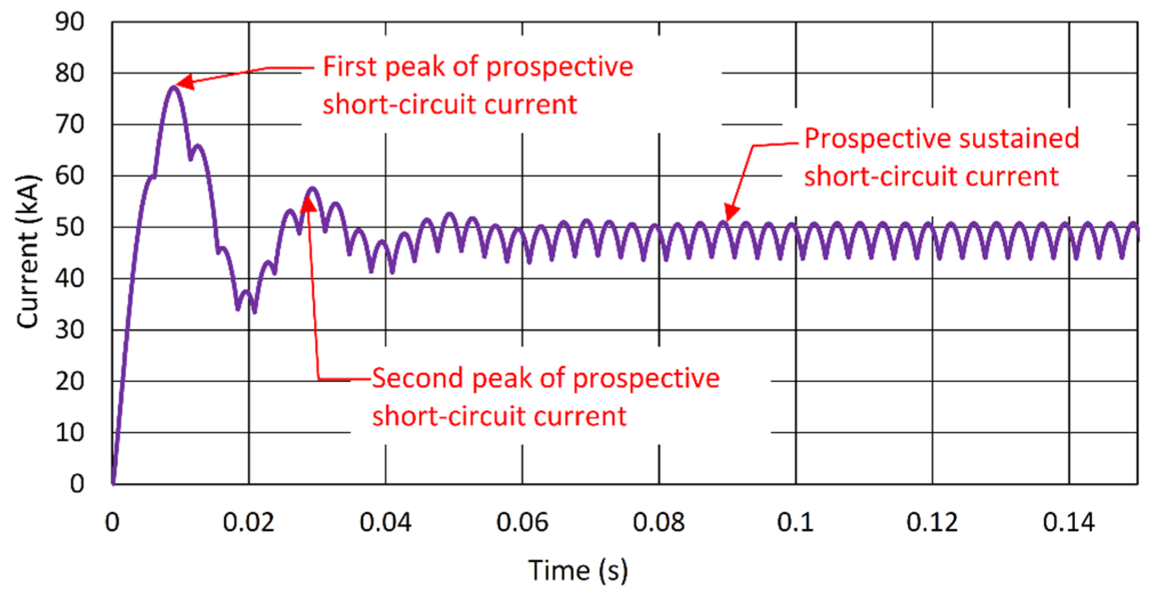
Figure 1 presents the short-circuit fault current in a 1500V DC rail system, measured at the DC circuit breaker of the transformer rectifier unit (TRU). The bolted fault was modeled in MATLAB/Simulink between the DC positive busbar and the negative busbar. The first peak of the short-circuit current had the highest value of the current and started to decay after 10 ms. The steady state of the short-circuit fault current was achieved after 60 ms.

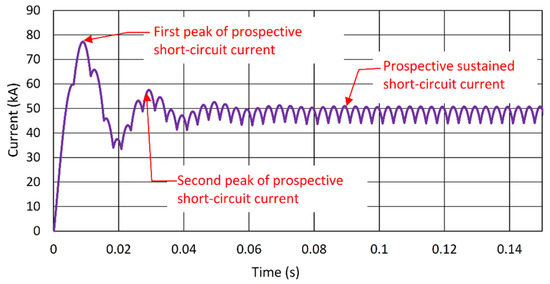
Figure 1. Bolted short-circuit fault current simulation results.

2.2. DC Protection

The role of the protection system is to isolate faulted circuits from all the electrical supplies in the event of a fault or abnormal operating condition [17]. The main type of protection used in a DC system are discussed below:

• Direct acting overcurrent protection (DAOC): DC high speed current limiting circuit breakers (fitted with a direct acting device) are used as main fault protection for the line feeder circuits [17]. The DC circuit breakers can detect and clear the fault between 15 and 20 ms. The setting parameter for the direct acting device is the minimum fault current that can be obtained from hand calculations [16] or fault modeling.
• Current rate of increase (di/dt) protection: To reduce unnecessary tripping and to discriminate between load and fault current, current rate of increase (di/dt) protection is used. The method is based on the fast rate of increase of the fault current wave compared with the load current. A fault current has a rate of increase of above 40 A/ms, where a load current is typical below 20 A/ms [12]. The load current rate of increase can be obtained from traction power modeling or assumed. The short-circuit fault current rate of increase can be calculated [16] or modeled with the help of specialized software.
• Frame leakage protection: DC substations use a floating ground, which means that the DC switchgear and rectifier cubicle are insulated from the ground. In the event of an insulation failure inside the DC switchgear or rectifier cubicle, the frame leakage detection will initiate the opening of all circuit breakers [17]. In practice, the minimum ground fault current setting value used for the frame leakage protection is 25 A.
• Over-voltage and under-voltage protection: Voltage relays are used to detect high-voltage or low-voltage conditions. The over-voltage and under-voltage limits used for relays settings can be sourced from EN 50,163 [18].

3. MATLAB/Simulink Modeling of the DC System with a Wayside Energy Storage Device

A light rail 1500 V DC traction power system was assumed for modeling purposes in MATLAB/Simulink (MathWorks). The power was distributed to trains from 1500 V DC substations using the overhead contact system. The current returns from trains to substations use train wheels and running rails. Because the rails are not perfectly insulated from the ground, some of the current will return to substations using ground and buried metalwork. This current is referred to earth leakage current or “stray current”.

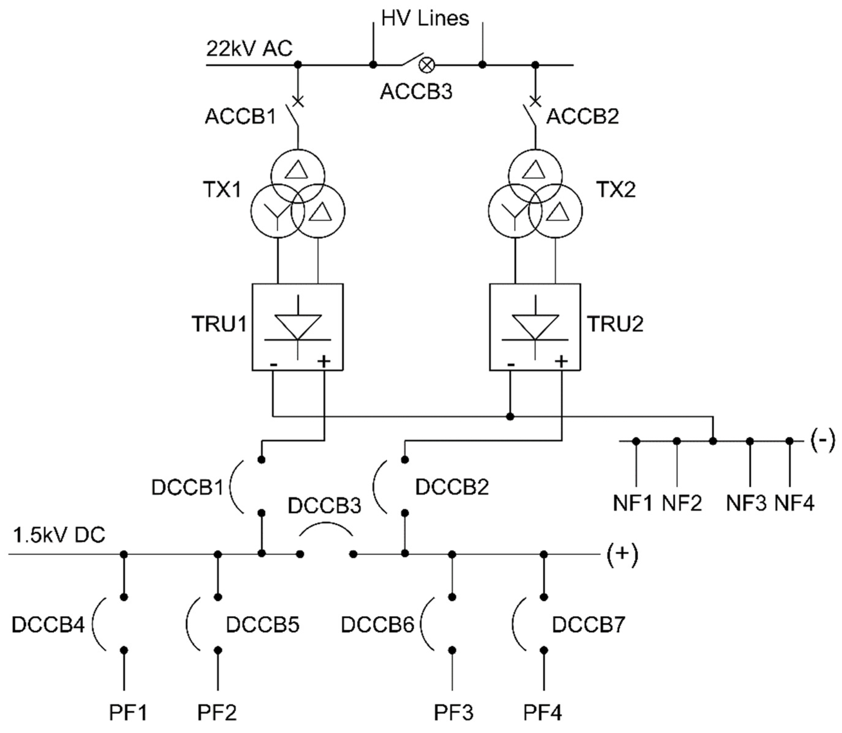
Figure 2 presents a typical 1500 V DC substation feeding arrangement. The substation is connected to the 22 kV AC distribution network operator (DNO) via HV lines. The OCS is fed from the substation transformer rectifier unit via DC circuit breakers and positive feeder cables (PF). In a normal feeding arrangement, the DC substation is equipped with two or more TRUs that feed in parallel with the OCS. The substation negative busbar is connected to the running rail via return negative feeders (NF). As there is no connection between the substation negative busbar and the ground, the system return is “floating”. The main reason that the negative return system is isolated from the ground is to minimize the earth leakage current and protect the buried metalwork. This may create touch potential issues along the route, as the rail-to-earth potential may rise. To provide a fault clearance path and to reduce rail-to-earth voltage, voltage limiting devices (VLDs) are installed along the route and at stations. EN 50122-1 provides guidance regarding touch potential limits [19]. British Standard (BS) 7671 provides guidance related to the touch potential clearance area [20].

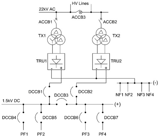
Figure 2. DC substation feeding arrangement.

In a DC traction power system, a trackside paralleling hut (TPH) is used to improve line voltage and to provide switching points between electrical sections. The TPH runs parallel with multiple tracks, and this reduces the longitudinal system impedance.

Figure 3 presents a TPH with a wayside energy storage device (WESD). The WESD with supercapacitors charges from the regenerative braking trains and boosts the line voltage when the line voltage is below a threshold value.

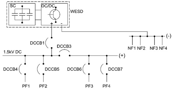
Figure 3. Trackside paralleling hut with a WESD.

The 1500V DC traction power system was divided in the following blocks to be modeled in MATLAB/Simulink:

• The substation block was divided into an HV source, a transformer, a rectifier, a positive feeder, and a negative feeder.
• A trackside paralleling hut block was equipped with a wayside energy storage device.
• OCS, running rails, and the earth block were also modeled.

3.1. Modeling of the Substation

The HV source was modeled in MATLAB/Simulink using a sinusoidal ideal voltage source. The AC voltage [21] is calculated as in Equation (1):

$$V=A \sin \left(\omega t+\varnothing \right)$$

(1)

where ∅ is the phase angle in radians, f is the frequency in Hz and ω is calculated as in Equation (2):

$$\omega =2\pi f$$

(2)

A three-phase system with an internal resistance and inductance can be modeled using three ideal voltage sources connected in Y with the neutral connection grounded. The source internal resistance and inductance were calculated from the internal impedance using the X/R ratio and short-circuit current. The short-circuit current and X/R ratio value were provided by the DNO. The ANSI standard IEEE C37.010 provided typical values for the transformer X/R ratios [22]. It is known that the higher the X/R ratio is, the longer the time constant is.

Table 1 presents the typical model input values calculated for the HV source block. The short-circuit current was assumed to be 13 kA, and the X/R ratio was assumed to be 7.

Table 1. HV source block model input values.

Parameter	Unit	Value
Voltage	kV	22
Short-circuit current	kA	13
X/R ratio	-	7
Source resistance (Rc)	Ω	0.1197
Source inductance (Lc)	H	0.0027

The rectifier transformer was modeled using a predefined MATLAB/Simulink three-phase transformer block. The primary transformer winding is connected in Δ, the first secondary winding is connected in Δ, and the second secondary winding is connected in Y. Values for the transformer rated power, voltage, current, and impedance can be sourced from the manufacturer data sheet. The simulation model requires values for the transformer magnetization resistance and inductance [18].

Equations (3) and (4) can be used to calculate per unit resistance and inductance for each winding [23].

$$R_{\left(pu\right)}=\frac{R\left(\Omega \right)}{R_{base}}$$

(3)

$$L_{\left(pu\right)}=\frac{L\left(H\right)}{L_{base}}$$

(4)

The base resistance and inductance can be calculated as in Equations (5) and (6) [23]:

$$R_{base}=X_{base}=\frac{V^2}{P}$$

(5)

$$L_{base}=\frac{X_{base}}{2\pi f}$$

(6)

An assumed magnetization current of 0.2% provides a magnetization resistance of 500 pu for the resistance and inductance.

Table 2 presents the transformer input parameters used for simulation purposes. The magnetization resistance and inductance were calculated with Equations (3)–(6).

Table 2. Transformer input parameters.

Parameter	Unit	Value (HV)	Value (LV1)	Value (LV2)
Rated voltage	V	22,000	581	581
Rated power	kVA	5000	2790	2790
Impedance	Ω	10.77	0.0145	0.0145
Resistance	Ω	0.46	0.00066	0.00066
Inductance	H	0.035	0.000046	0.000046
Connection	-	D	D	Y
Frequency	Hz	50
Magnetization resistance	Ω	44,856.35
Magnetization inductance	H	142.78

A 12-pulse diode rectifier was modeled using diode blocks with internal resistance and diode forward voltage parameters. Each diode was equipped with a capacitor connected in parallel. At the output of the rectifier, a capacitor was connected in parallel to provide a steady voltage. The rectifier parameters were sourced from manufacturer data sheets.

Figure 4 presents the HV source and the transformer rectifier blocks that were modeled in MATLAB/Simulink.

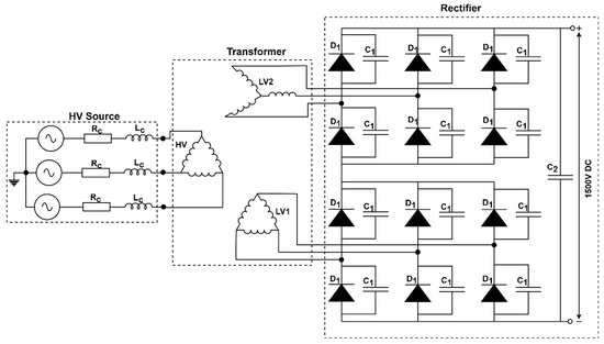
Figure 4. HV source and transformer rectifier modeled in MATLAB/Simulink.

The diode internal resistance and forward voltage was sourced from [24]. The diode parallel capacitor and rectifier output capacitor were sized with a trial-and-error method (Table 3). These values can be sourced from the rectifier manufacturer data sheet.

Table 3. Rectifier input parameters [24].

Parameter	Unit	Value
Rated voltage	V	1500
Rated power	MW	4
Pulse number	-	12
Diode internal resistance (Ri)	mΩ	0.063
Diode forward voltage (D1)	V	1.05
Diode parallel capacitor (C1)	mF	0.0001
Rectifier output capacitor (C2)	mF	0.1

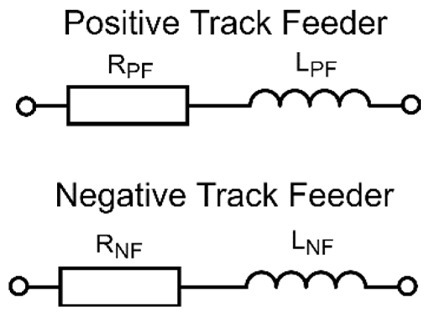
Figure 5 presents the positive and negative feeder blocks that were modeled in MATLAB/Simulink. The positive feeder was modeled using a resistance (R_PF) connected in parallel with an inductance (L_PF). The negative feeder was modeled similarly using a resistance (R_NF) connected in parallel with an inductance (L_NF).

Figure 5. Substation positive and negative feeders modeled in MATLAB/Simulink.

The resistance and inductance for the positive feeder and the negative feeder were sourced at a temperature of 20 °C, based on the manufacturer data sheet. Depending on the geographic area where the traction power system was located, the resistance and inductance were calculated for a temperature between 45 and 60 °C, taking into consideration the traction current.

Table 4 presents the resistance and inductance value calculated for the substation positive feeder cable and the negative feeder cable according to BS IEC 60287-2-1:2015 [25].

Table 4. Positive feeder and negative feeder cable input parameters [26].

Parameter	Unit	Value
Negative feeder cable type	-	1C 300 mm2 3.8/6.6 kV, Al, XLPE/HDPE
Positive feeder cable type	-	1C 500 mm2 3.8/6.6 kV, Al, XLPE/HDPE
Initial temperature	°C	20
Final temperature	°C	45
Negative feeder resistance at final temperature (RNF)	Ω/km	0.12
Negative feeder inductance at final temperature (LNF)	H/km	0.000315
Positive feeder resistance at final temperature (RPF)	Ω/km	0.071
Positive feeder inductance at final temperature (LPF)	H/km	0.000305

3.2. Trackside Paralleling Hut with Wayside Energy Storage Device

The trackside paralleling hut was modeled similar to the substation block described in Section 3.1. The trackside paralleling hut was equipped with a positive and negative busbar to provide a paralleling point and supply continuity from the WESD to the tracks. The WESD was modeled with the MATLAB/Simulink supercapacitor block and Cuk converter arrangement standards described in [27].

To protect the WESD from a high fault current, the maximum load/fault current was limited to 3000 A. Resistance and inductance ‘RL’ MATLAB/Simulink blocks were connected in series with the WESD. The resistance was calculated as 0.523 Ω, and the inductance was assumed to be 6 mH.

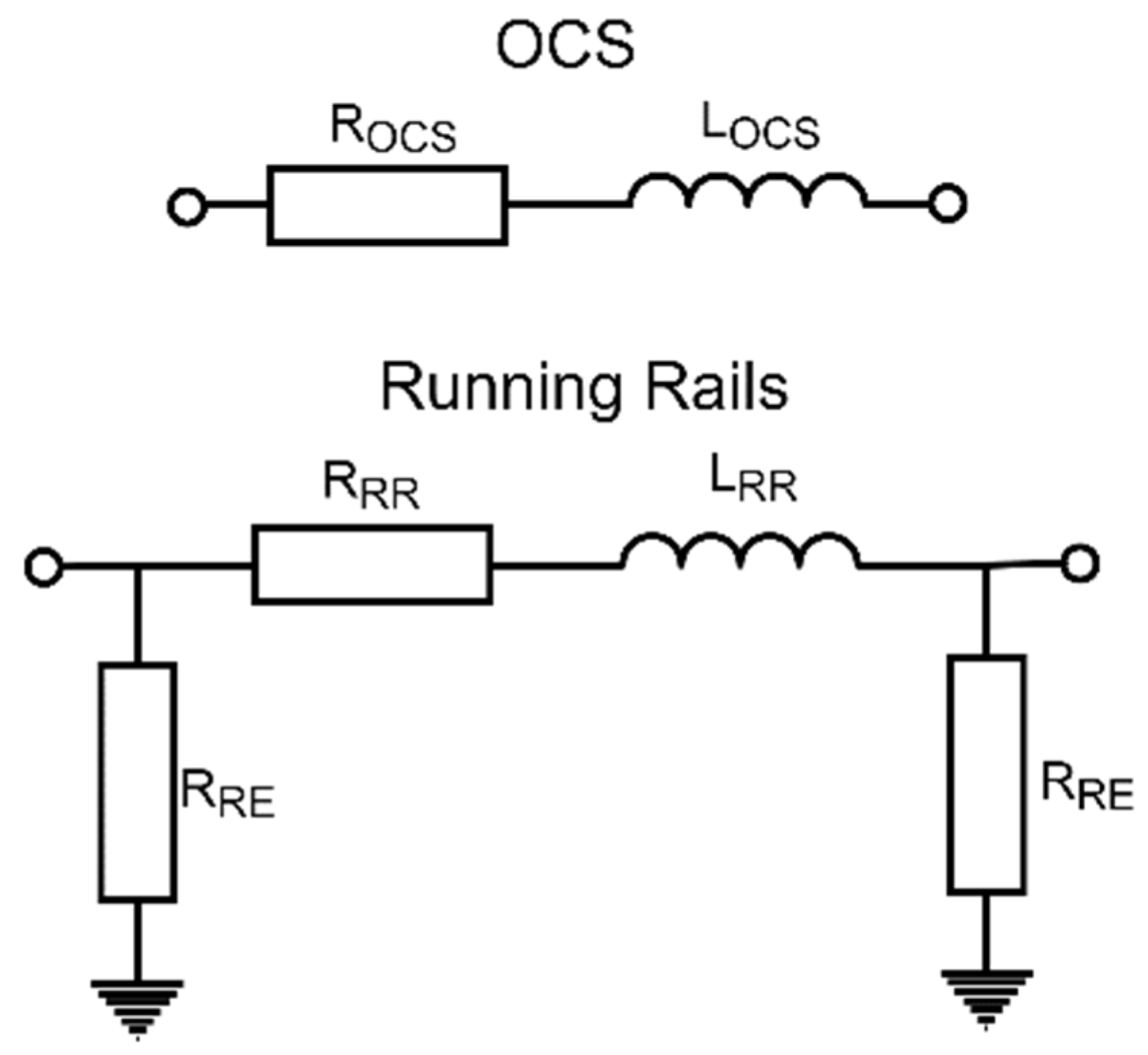
3.3. Modeling of the OCS, Running Rail, and Earth

The OCS was modeled using a resistance connected in parallel with an inductance. Typical OCS resistance (R_OCS) and inductance (L_OCS) values (Ω/km and H/km) were sourced at a temperature of 20 °C, based on the manufacturer data sheet. Depending on the geographic area where the traction power system was located, the resistance and inductance were calculated for a temperature between 45 and 60 °C, taking into consideration the traction current. The contact wire wear was normally assumed to be 30% of the new contact wire.

The track feeders, the OCS, and the rail inductance L (mH/km) can be calculated as in Equation (7):

$$L=0.2\left(ln\frac{2000}{R}-0.75\right)$$

(7)

where R is the radius of the conductor, measured in meters:

$$R=\sqrt{\frac{A}{\pi }}$$

(8)

The running rail resistance (R_RR) and inductance (L_RR) were modeled like the OCS. The wear for the rail is normally assumed to be 20% from the top of the rail. A common assumption in traction power modeling projects is that the top of the rail is 1/3 of the rail. The rail-to-earth resistance (R_RE) is approximative 100 Ω·km for a new railway system and drops to 10 Ω·km after a period of usage [13]. For the signaling system to work, the rail-to-earth resistance is normally required to be above 2–3 Ω·km.

Figure 6 presents the OCS and running rails blocks that were modeled in MATLAB/Simulink.

Figure 6. OCS and running rails modeled in MATLAB/Simulink.

Table 5 summarizes the OCS and running rail input parameters. The OCS/rail resistance and inductance at a final temperature of 45 °C were calculated as in [15]. The input parameters for the temperature calculations were similar to the one used in [15].

Table 5. OCS and running rail input parameters.

Parameter	Unit	Value
Running rail type	-	UIC 60
OCS configuration	-	1 × Contact Wire 161 mm2 + 1 × Catenary Wire 181 mm2
Rail wear	%	20
Contact wire wear	%	30
Initial temperature	°C	20
Final temperature	°C	45
OCS resistance at final temperature with wear (ROCS)	Ω/km	0.072
OCS inductance at final temperature with wear (LOCS)	H/km	0.0023
Rail resistance at final temperature with wear (RRR)	Ω/km	0.039
Rail inductance at final temperature with wear (LRR)	H/km	0.0011
Rail to earth resistance (RRE)	Ω.km	10

3.4. Model Validation

A validation was conducted to compare the short-circuit fault current calculated from the proposed MATLAB/Simulink model with the values obtained from hand calculations according to EN 50123-1 [16].

For the validation exercise, the following input data was used:

• a single track 1500 V DC system with a single 4 MW TRU substation (for substation parameters, see Table 2 and Table 3);
• DC substation negative and positive feeders with a length of 50 m (for cable parameters, see Table 4);
• a track length of 1 km (the OCS and running rail resistance are presented in Table 5);
• a bolted fault between the OCS and the running rail that was assumed to be 1 km away from the substation (Figure 7).
  

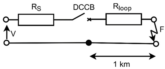  Figure 7. Equivalent circuit of the test model.

Table 6 presents the calculated equivalent source resistance and loop resistance. The loop resistance includes the positive feeder, negative feeder, OCS, and single running rail resistance.

Table 6. Test model input parameters.

Parameter	Unit	Value
DC supply voltage (U)	V	1570
Equivalent source resistance (Rs)	mΩ	41.98
Loop resistance between substation and fault location $(R_{loop})$	mΩ	120.6
Fault location	km	1

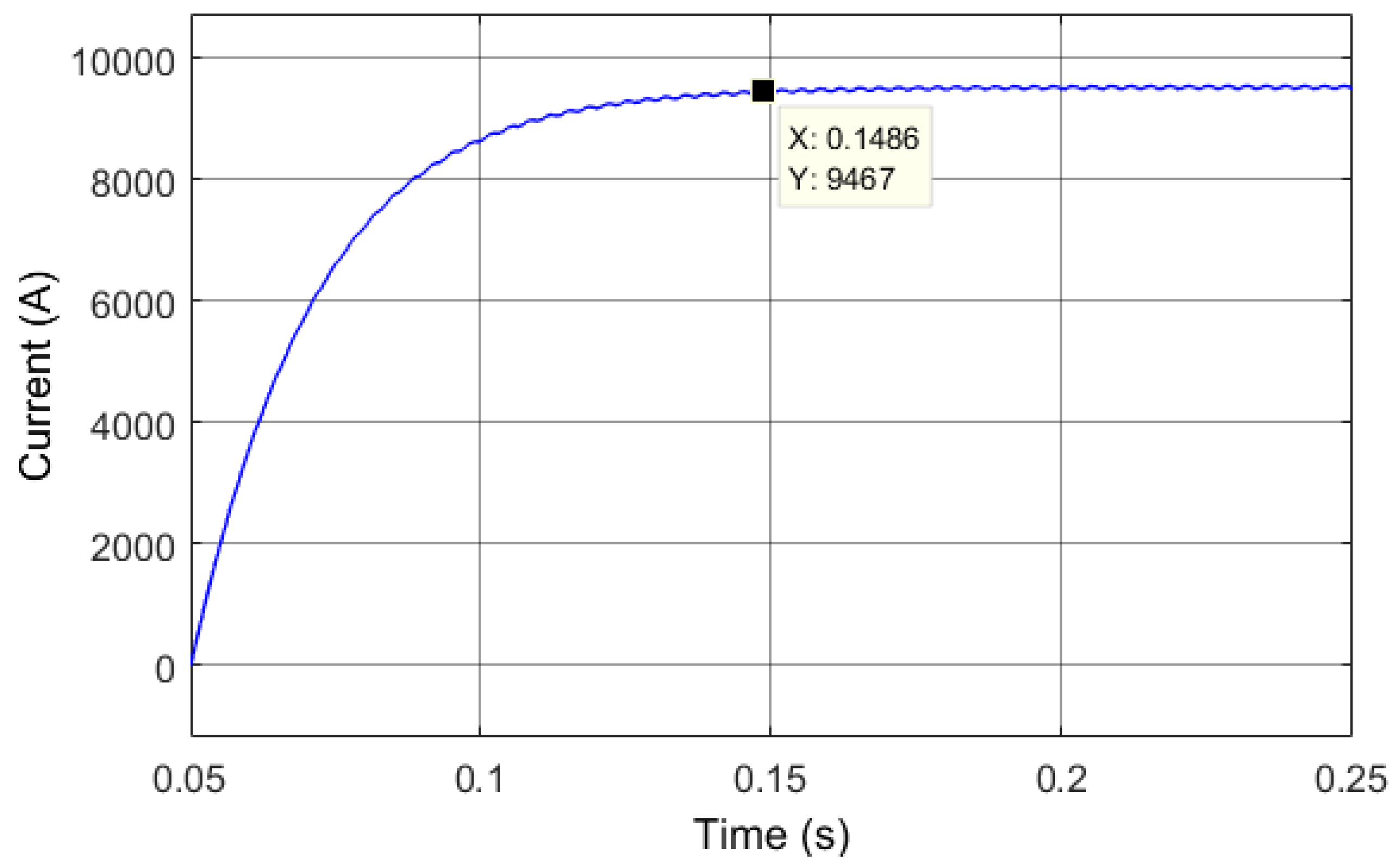
The bolted short-circuit fault current contribution (I_F) from the substation can be calculated with Equation (9):

$$I_F=\frac{U}{R_s+R_{loop}}$$

(9)

Figure 8 presents the MATLAB/Simulink calculation result of the 9.467 kA short-circuit bolted fault current. The fault current is a distant short-circuit fault current simulated to be 1 km from the analyzed substation.

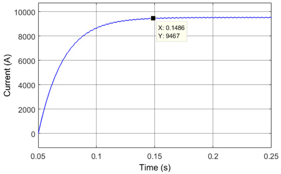
Figure 8. Test model simulation results.

Table 7 presents the simulation and hand calculation results. The approximation error between the two set of the results was calculated. The results below show that the relative error was 1.02% for the modeled short-circuit current, which provides a good validation of the proposed MATLAB/Simulink model.

Table 7. Short-circuit fault current results.

Parameter	Unit	Value
MATLAB/Simulink short-circuit fault current	A	9467
Short-circuit fault current calculated with Equation (9)	A	9660
Relative error	%	1.02

4. Case Study

4.1. Modeling Input Data

This section presents the input data used for traction power modeling in Modeltrack [14,15] and the short-circuit study using the MATLAB/Simulink model described in Section 3.

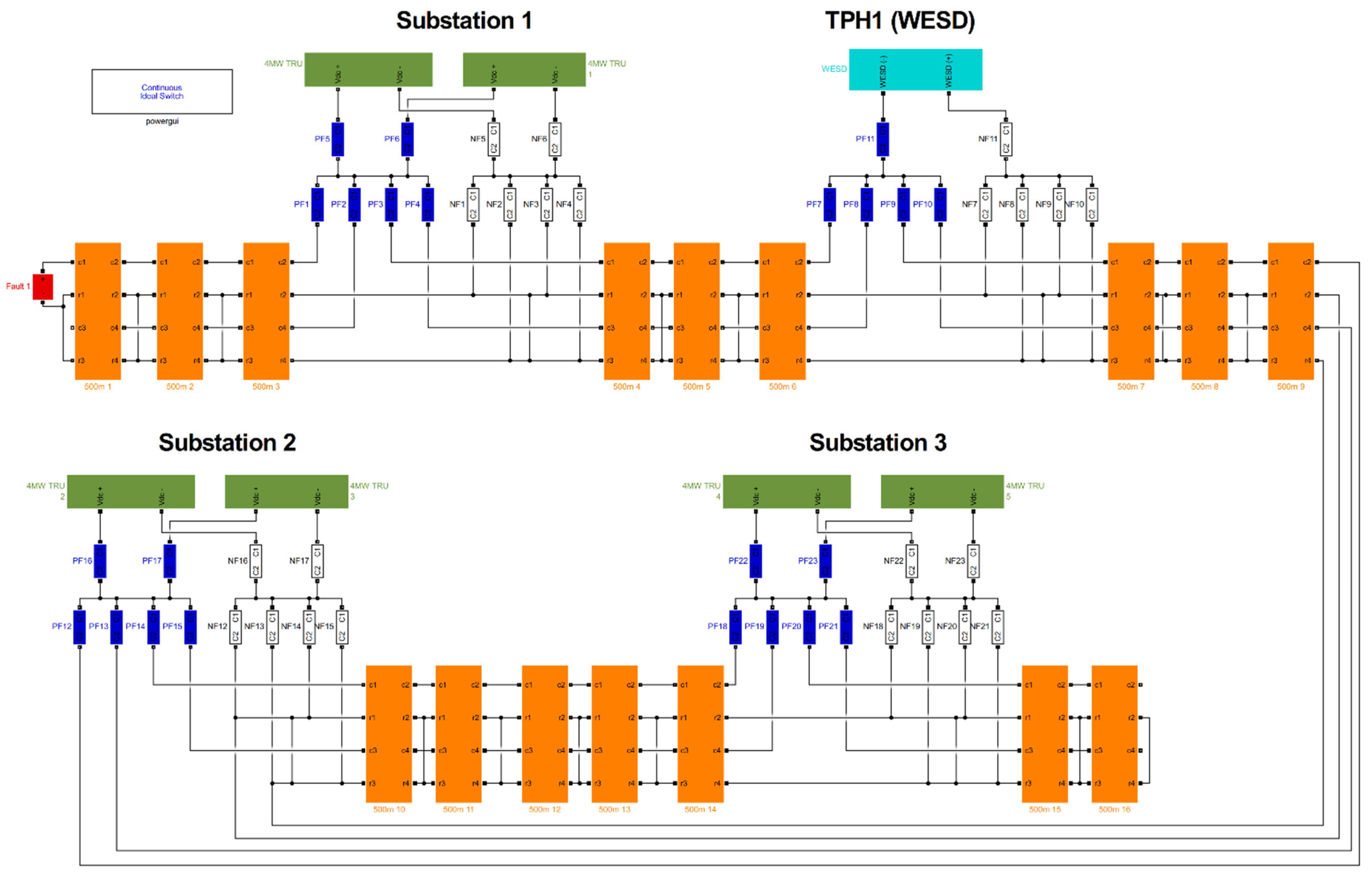
An 8 km light railway 1500V DC traction power system was modeled (Figure 9). DC substations are shown in green, the TPH in turquoise, positive track feeders in blue, negative track feeders in black, the fault block in red, and the OCS and running rail block in orange. The cross bonds are evenly spaced every 500 m. The traction power system blocks are described in Section 3.

Figure 9. MATLAB/Simulink model of the 1500V DC traction power system.

The system consists of three DC substations (Table 8), one TPH with a WESD (Table 9), and six stations (Table 10). Each substation is equipped with a 2 × 4 MW TRU. The WESD has a capacity of 40 MJ and a maximum charging/discharging current of 3000 A.

Table 8. Substation input parameters.

Substation No.	Nominal Voltage (V)	No Load Voltage (V)	TRU No. and Rating (MW)	Location (m)
Substation 1	1500	1570	2 × 4	1500
Substation 2	1500	1570	2 × 4	4500
Substation 3	1500	1570	2 × 4	7000

Table 9. TPH with WESD input parameters.

Parameter	Unit	Value
Location	m	3000
Capacity	MJ	40
Nominal voltage	V	1500
Efficiency (supercapacitor and DC/DC converter)	%	95
Max. charging/discharging current	A	3000
Initial state of charge	%	100

Table 10. Station input parameters.

Station No.	Location (m)	Dwell Time (s)
Station A	0	60
Station B	1500	60
Station C	3000	60
Station D	4500	60
Station E	7000	60
Station F	8000	60

Table 11 present typical train parameters assumed for simulation purposes. A headway of 180 s with a station dwell time of 60 s is assumed.

Table 11. Train input parameters.

Parameter	Unit	Value
Number of units	-	8
Unit length	m	20
Unit weight	tonnes	58
Payload	tonnes	7
Voltage	V	1500
Maximum tractive effort	kN	270
Maximum acceleration rate	m/s2	1
Mean braking service rate	m/s2	1
Davis coefficient k1	-	0.006434
Davis coefficient k2	-	0.025633
Davis coefficient k3	-	12
Rotating mass factor	-	1.08

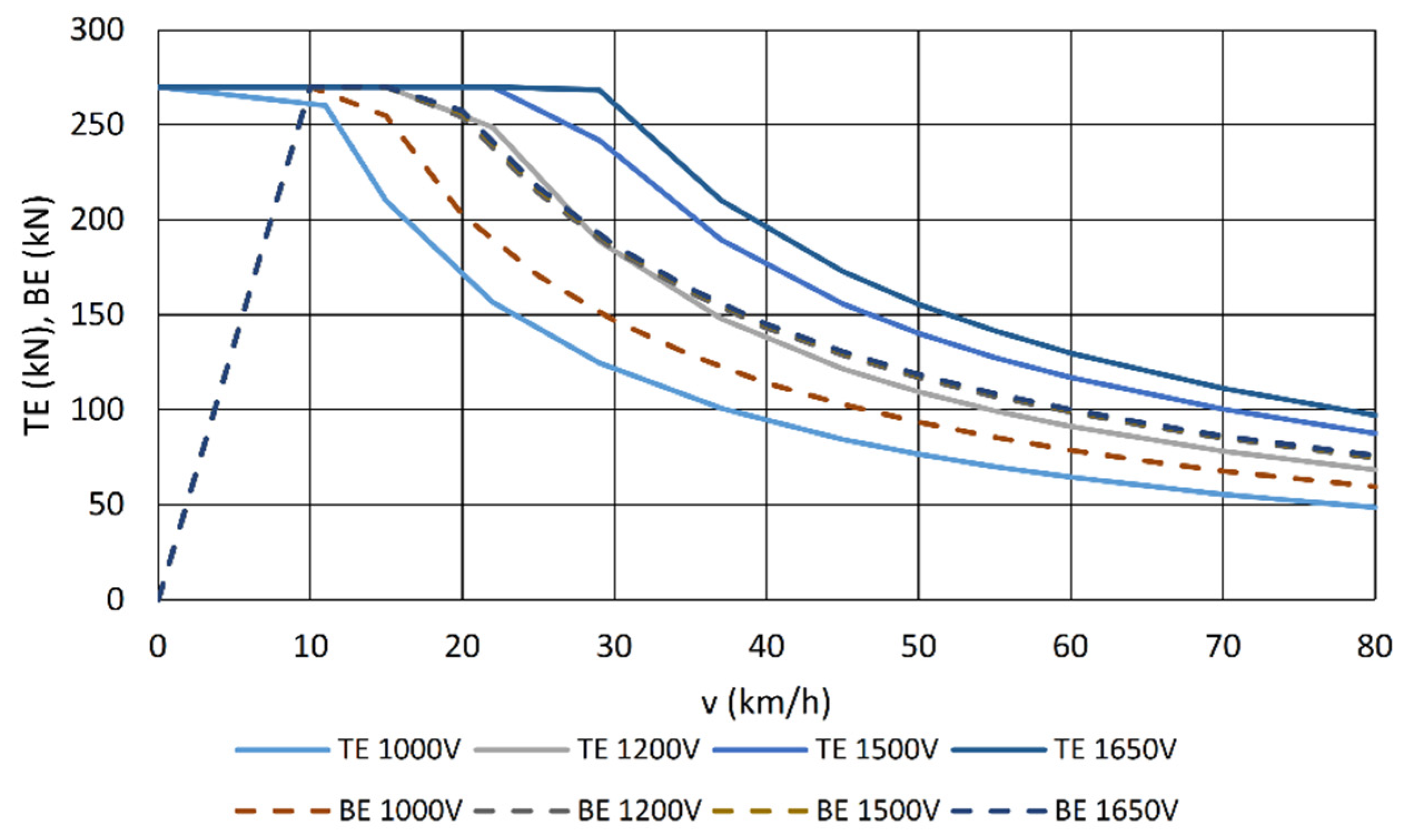
Figure 10 presents assumed train tractive effort (TE) and braking effort (BE) curves as a function of velocity (v). The braking effort curves for 1000 V and 1500 V have similar values, as do those of the braking effort curves for 1200 V and 1650 V. The line voltage difference has a greater impact on the tractive effort curves compared with the braking effort curves.

Figure 10. Train tractive effort and braking effort as a function of velocity.

4.2. Traction Power Modeling Simulation Results

The electrified transportation system model can be divided into two parts: In the first part, the train mechanical calculations were conducted as presented in [14], and the second part consists of the electrical network solver, described in [15].

The simulation results presented in Table 12 show that the highest load current feed to the OCS is from DC Circuit Breaker 4 (DCCB4), Substation 2.

Table 12. Traction power modeling simulation results.

Substation No.	Max. 1 s RMS Current DCCB4 (A)	Max. 1 s RMS Current DCCB5 (A)	Max. 1 s RMS Current DCCB6 (A)	Max. 1 s RMS Current DCCB7 (A)
Substation 1	3000	2888	1998	4022
TPH 1 (WESD)	2612	1559	1947.4	2183
Substation 2	4051	1716	2732	3020
Substation 3	3002	3000	1821	3000

Figure 11 presents the simulation results for Substation 1, DCCB5 and DCCB7.

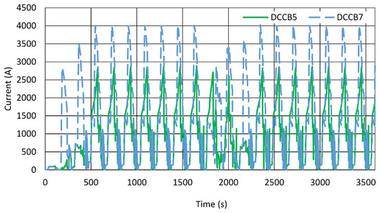
Figure 11. Simulation results for Substation 1—current vs. time feed to the OCS of DCCB5 and DCCB7.

It can be concluded from Table 13 that the highest loaded substation in the system is Substation 1.

Table 13. TRU CB simulation results.

Substation No.	Max. 1 s RMS Current DCCB1 (A)	Max. 1 s RMS Current ACCB1 (A)
Substation 1	4154	356
Substation 2	3909	335
Substation 3	3502	300

4.3. Short-Circuit Fault Current Simulation Results

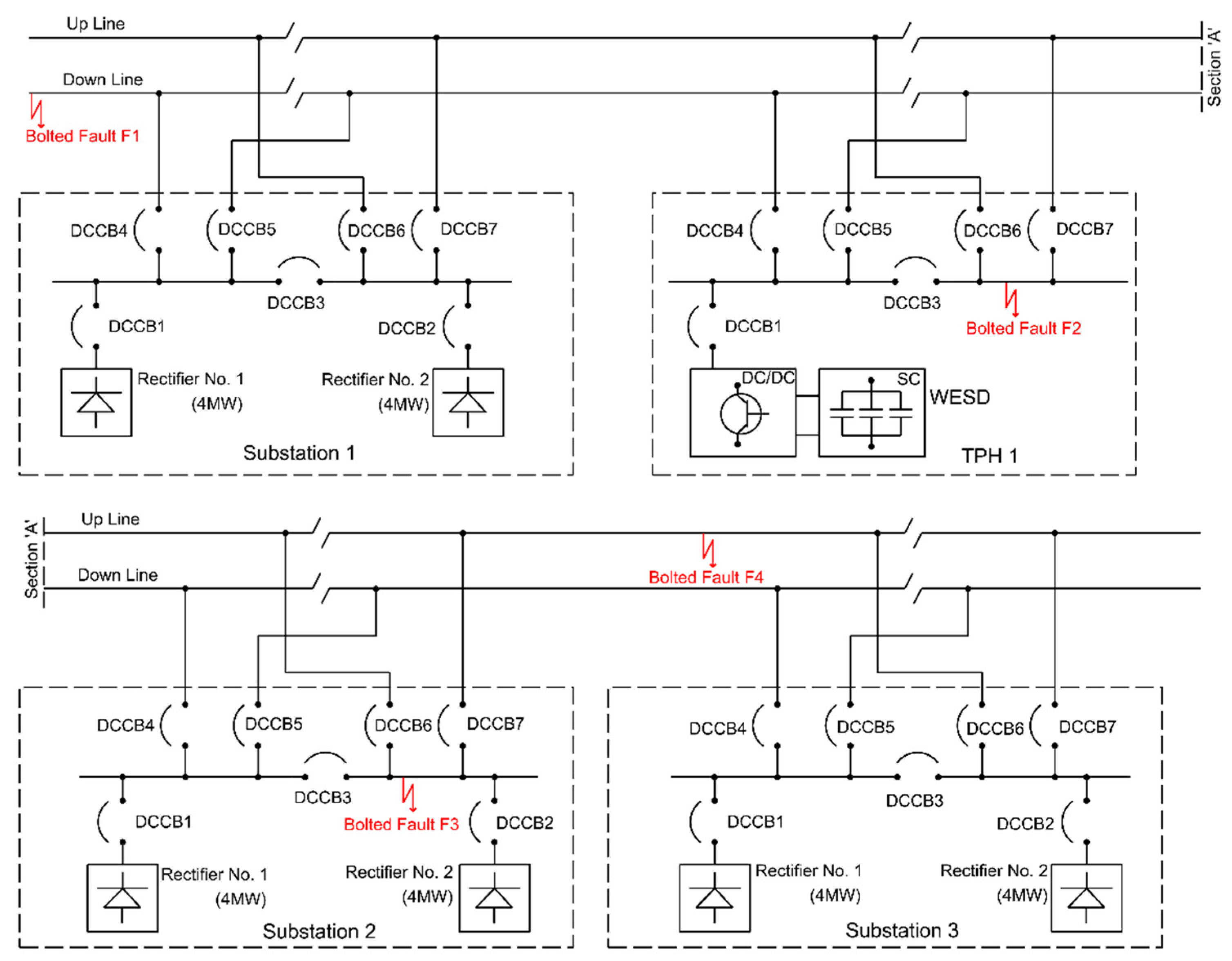
In the MATLAB/Simulink model, four different scenarios were simulated to analyze the magnitude of the fault currents (Figure 12). Each scenario below was modeled individually:

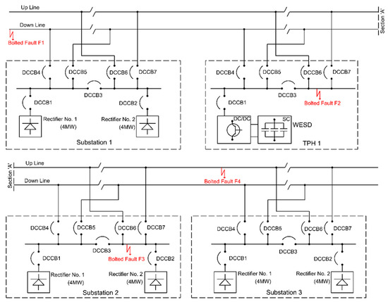
Figure 12. Fault scenarios modeled in MATLAB/Simulink.

• Scenario F1: The F1 scenario assumes a bolted fault between the contact wire and the rail on the down line (at the start of the line).
• Scenario F2: The F2 scenario assumes a bolted fault between the 1500 V DC WESD positive busbar and the negative busbar.
• Scenario F3: The F3 scenario assumes a bolted fault between the 1500 V DC positive busbar and the negative busbar at the Substation 2 busbar.
• Scenario F4: The F2 scenario assumes a bolted fault between the contact wire and the rail on the up line (1.5 km from Substation 2).

In all four scenarios, the DC circuit breakers are closed for all substations and the TPH. This means that each substation TRU feeds the railway system in parallel.

Table 14 presents the maximum short-circuit fault current and the current rate of increase results for the modeled scenarios. The results were chosen to show the fault current on the DC circuit breaker on each side of the fault.

Table 14. Bolted fault simulation results.

Substation No.	DCCB ID	Max. Fault Current (A)	di/dt (A/ms)	Fault Scenario
Substation 1	DCCB1	3905	28	F1
Substation 1	DCCB2	3905	28	F1
Substation 1	DCCB4	9239	66	F1
TPH 1 (WESD)	DCCB4	714	5	F1
TPH 1 (WESD)	DCCB1	2906	40	F2
TPH 1 (WESD)	Busbar	34,530	241	F2
Substation 1	DCCB5	7608	76	F2
Substation 2	DCCB4	8021	83	F2
Substation 2	DCCB2	33,950	999	F3
Substation 2	Busbar	88,270	849	F3
Substation 3	DCCB6	4888	74	F3
TPH 1 (WESD)	DCCB7	4888	74	F3
Substation 2	DCCB7	9163	72	F4
Substation 3	DCCB6	12,280	83	F4

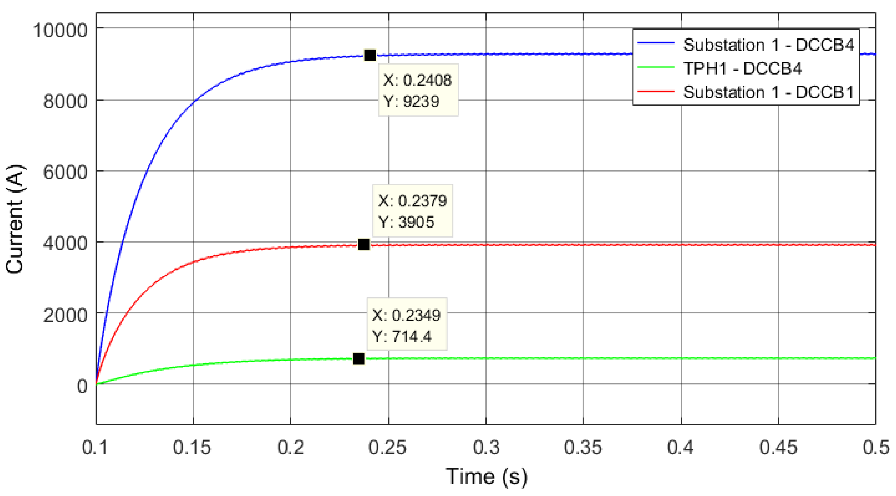
F1 models a bolted fault between the OCS down line and the running rail. Figure 13 shows that the highest current (9.24 kA) was found in DCCB4 of Substation 1. The transformer rectifier unit (DCCB1) of Substation 1 only feeds 3.9 kA. The remainder of the fault current is fed by the second TRU and other substations/TPH WESD in the system.

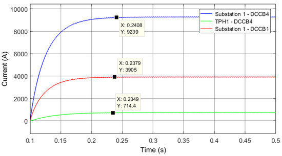
Figure 13. Simulation results of Scenario F1. Fault current (A) vs. time (s) observed with the DCCB4 (Substation 1—blue), DCCB1 (Substation 1—red), and DCCB4 (TPH1—green).

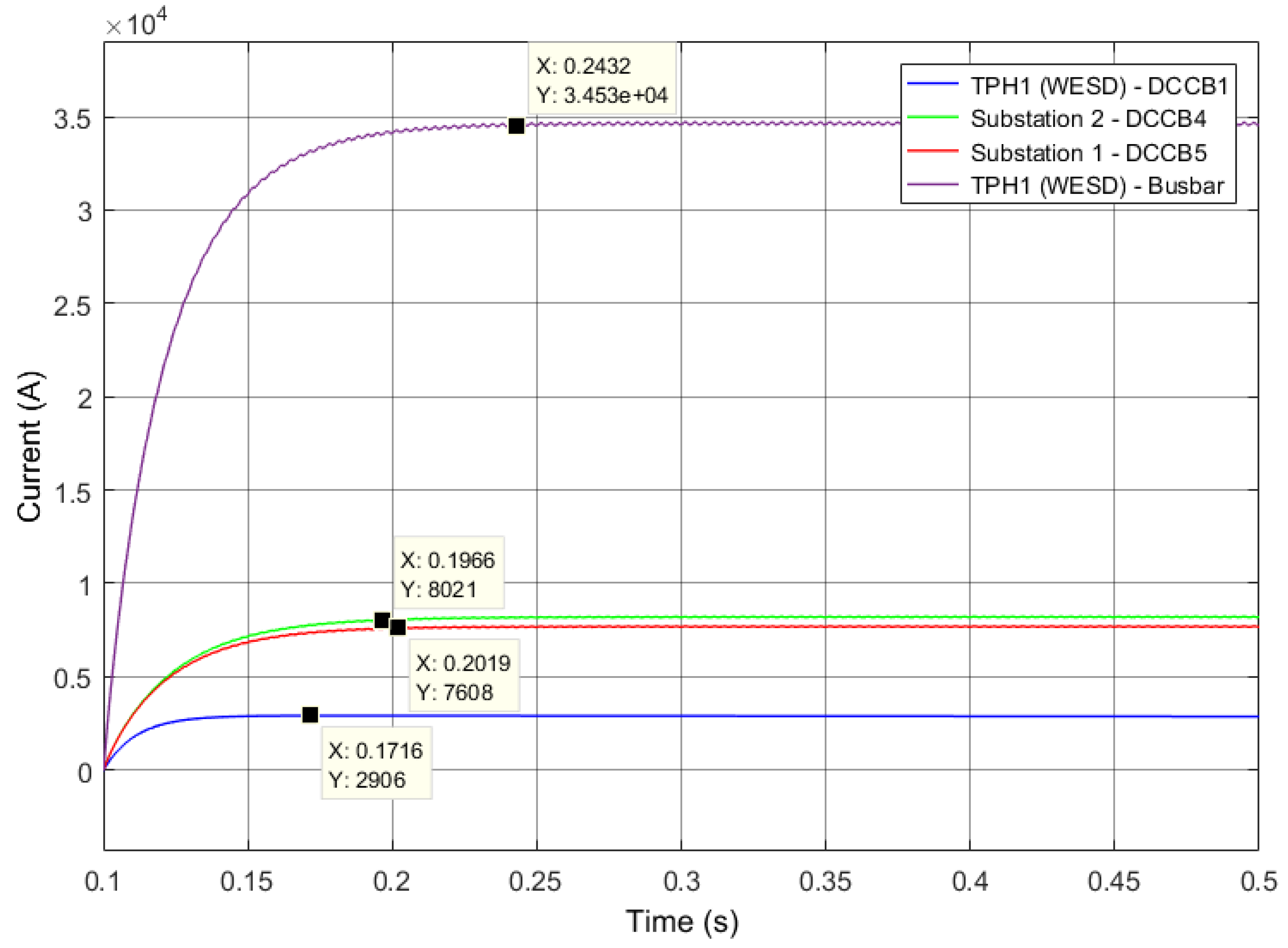
F2 modeled a bolted fault at the TPH DC busbar. Figure 14 shows that the short-circuit maximum value at the DC busbar had a value of 34.5 kA.

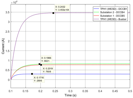
Figure 14. Simulation results of Scenario F2. Fault current (A) vs. time (s) observed with DCCB1 (TPH 1—blue), DCCB4 (Substation 2—green), DCCB5 (Substation 1—red), and TPH1 busbar (violet).

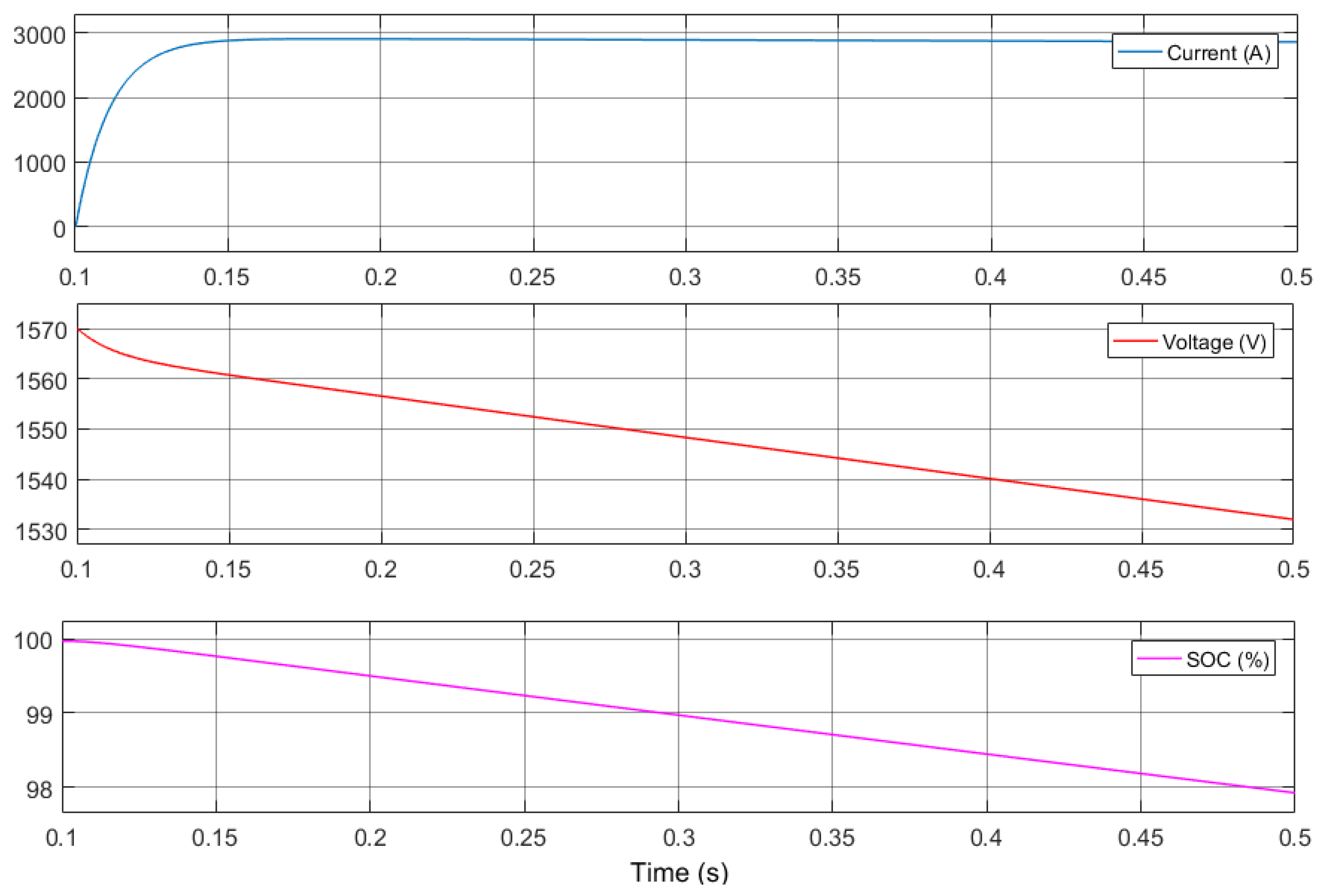
Figure 15 shows that the WESD feeds approximately 3 kA to the fault. The state of charge (SOC) of the WESD SC cells drops at 0.4 s from 100% to below 98%.

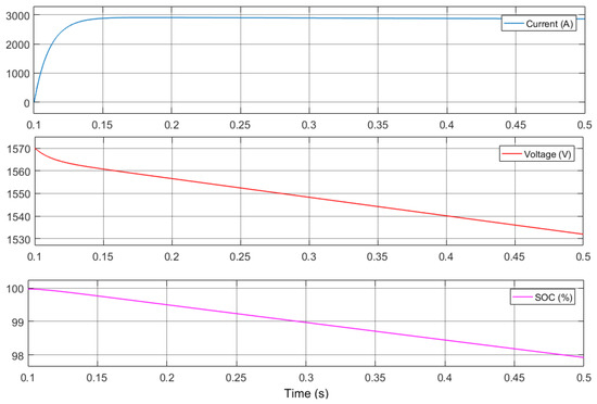
Figure 15. Simulation results WESD Scenario F2. Fault current (A), voltage (V), and SOC (%) vs. time (s).

F3 modeled a bolted fault at the Substation 2 DC busbar. Figure 16 shows that the first peak of the prospective short-circuit current under transient conditions at the Substation 2 DC busbar had a value of 81.58 kA. The prospective sustained current that results from the short-circuit had a value of 88.27 kA at the Substation 2 DC busbar. This difference in fault current values is caused by circuit reactance.

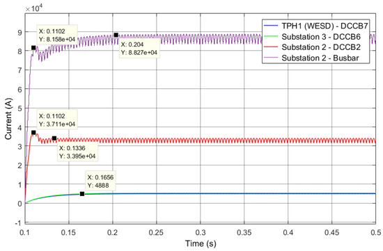
Figure 16. Simulation results of Scenario F3. Fault current (A) vs. time (s) observed with DCCB7 (TPH 1—blue), DCCB6 (Substation 3—green), DCCB2 (Substation 2—red), and the Substation 2 busbar (violet).

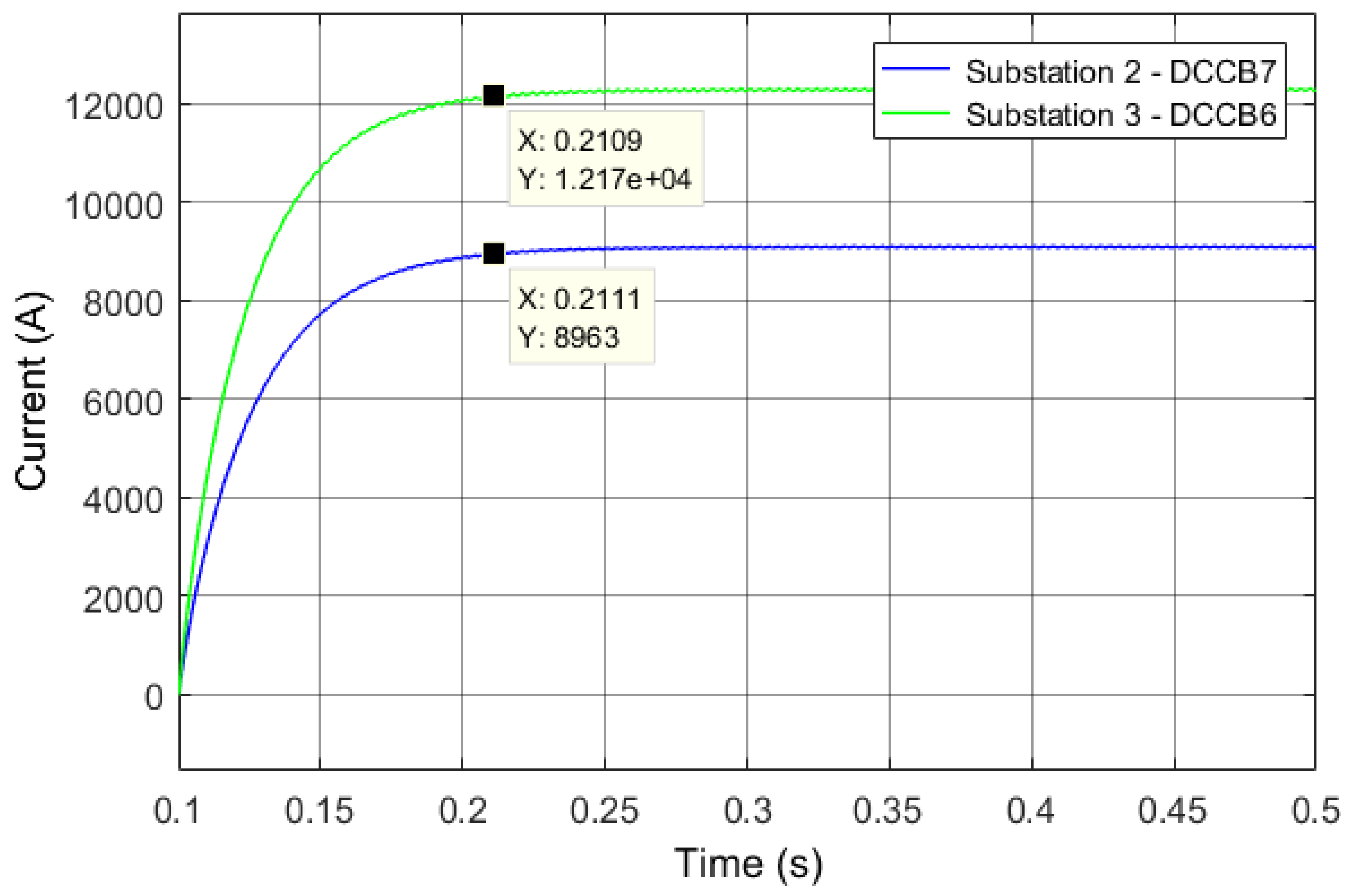
F4 modeled a bolted fault between the OCS up line and the running rail. Figure 17 shows that the highest current (12.17 kA) is fed by the DCCB6 of Substation 3. The DCCB7 of Substation 2 feeds 8.96 kA due to the longer feeding length in relation to the fault (distance from Substation 2 to the fault = 1.5 km; distance from Substation 3 to the fault = 1 km).

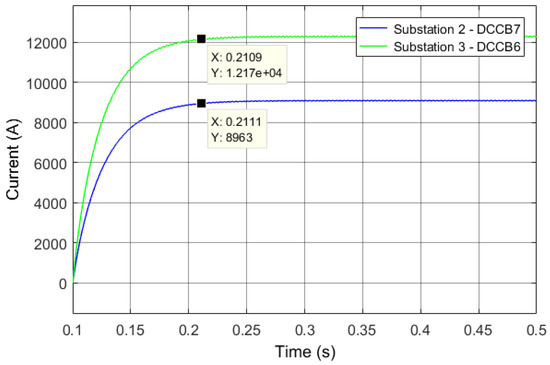
Figure 17. Simulation results of Scenario F4. Fault current (A) vs. time (s) observed with DCCB7 (Substation 2—blue) and DCCB6 (Substation 3—green).

4.4. DC Protection Analysis

Traction power simulations were conducted in Modeltrack to determine the maximum current flowing in each DCCB (Section 4.2). To account for multiple trains accelerating in the same electrical section, an allowance of +20% on top of the maximum instantaneous load current was assumed.

The MATLAB/Simulink model was used to conduct fault current analysis. For protection analysis, the minimum fault current that could be observed with the DCCB track feeders, described in Section 4.3, was calculated. An allowance of −10% was assumed for the minimum calculated DC fault current (Table 15).

Table 15. Track feeder protection analysis.

Sub. No.	DCCB ID	Min. Fault Current (A)	Max. Load Current (A)	DAOC Setting Range (A)	Fault Current Detectable	di/dt (A/ms)	Fault Scenario
Sub. 1	DCCB4	8315	3600	3601 → 8315	Yes	66	F1
Sub. 2	DCCB7	8247	3624	3625 → 8247	Yes	72	F4
Sub. 3	DCCB6	11,052	2185	2186 → 11052	Yes	83	F4

From Table 15, it can be concluded that the direct acting overcurrent protection will trip the DC circuit breaker in an event of a minimum fault current that can be distinguished from the maximum load current. The di/dt protection can be implemented, as the fault current rate of increase is well above 20 A/ms (the assumed maximum current rate of increase for the load current). In [12], the current rate of increase recognition threshold was set to 30 A/ms. The measured train load values for the current rate of increase were below 10 A/ms.

4.5. DC Circuit Breaker Withstand and Breaking Capacity Analysis

The short-circuit fault simulation results in Section 4.3 were used to assess the withstand and breaking capacity of the DC circuit breaker for the maximum current and distant fault. For the fault assessment, it was assumed that the substations are equipped with an Alstom ARC1550 DC circuit breaker. The DC circuit breaker breaking capacity data taken from the manufacturer data sheet is presented in Table 16 [28].

Table 16. Alstom ARC1550 DCCB breaking capacity data [28].

Rated Short-Circuit Current (INss) (kA)	Rated Track Time Constant (TNc) (ms)	Voltage (V)
102	2	1500
68	15	1500
55	30	1500
50	75	1500

Table 17 considers two types of faults (close and distant fault) to assess the impact of the short-circuit fault current on the withstand and braking capability of the Alstom DC circuit breaker. In Scenario F3 (where the fault is located at Substation 2’s DC busbar), the maximum fault current, which considers the contribution from all substations in the system, is 88.27 kA. The track time constant was calculated to be 4.3 ms. If we compare the fault simulation results with the DC circuit breaker manufacturer data, we can observe that, for the 4.3 ms time constant, the DC circuit breaker withstand capability is 97 kA, which means that the DC circuit breaker is correctly rated.

Table 17. DC circuit breaker withstand and breaking capacity assessment.

Fault Scenario	Fault Location	INss ARC1550 (kA)	TNc ARC1550 (ms)	${\widehat{\mathbf{I}}}_{\mathbf{S}\mathbf{S}}(\mathbf{kA})$	TC (ms)
F1	Down Line, 0 km	28.5	87.9	9.2	87.9
F3	Substation 2, DC busbar	97	4.3	88.27	4.3

For the distant fault (F1), the highest fault current was 9.2 kA with a track time constant of 87.9 ms. The track time constant had a higher value in this case because it included the OCS as well as the running rail resistance and inductance. The DCCB could withstand a current of 28.5 kA at a time constant of 87.9 ms, which proves that the DCCB is correctly rated.

5. Conclusions

The MATLAB/Simulink model developed for fault modeling in DC systems is a useful tool to model different types of DC short-circuit faults: distant, close, bolted, and arc short-circuit faults. The paper presents a method to model substations, trackside paralleling huts, wayside energy storage devices, track feeders (positive and negative), overhead contact systems, running rails, and rail-to-earth resistance in MATLAB/Simulink. The proposed model eliminates the over-simplification of existing short-circuit models by taking the parameters that have a direct impact on the magnitude and shape of the fault current into consideration. A validation of the software according to EN 50123-1 [11] was conducted with good results, showing a 1.02% relative error.

Results of the case study using the MATLAB/Simulink model for a 1500 V DC light rail system show that the maximum short-circuit current for a bolted fault at the DC positive busbar is 88.27 kA (F3). The analyzed Alstom circuit breaker can withstand 97 kA at a time constant of 4.3 ms. The distant fault (F1) shows a maximum short-circuit fault current of 9.2 kA. At a track time constant of 87.9 ms, the Alstom circuit breaker can withstand 28.5 kA. The simulation results demonstrate that the circuit breaker is correct rated for the analyzed system (Table 17).

In [6], a fault modeled 50 m from a DC substation (2 MVA TRU) had a short-circuit current peak of 33 kA. In this paper, the substations were equipped with a 2 × 4 MW TRU, and the close fault was modeled at the substation DC busbar, which provided a higher fault current. In another study, the peak of the short-circuit current for the distant bolted fault was 3.6 kA [12], comparable to the value modeled in this paper, i.e., 3.9 kA (F1, Table 14).

The WESD maximum load and fault current was limited to 3000 A to protect the equipment. The WESD fault contribution was marginal compared with the substation fault contribution located adjacent to the fault location.

Protection analysis was conducted to determine if direct acting overcurrent protection can distinguish between the maximum load current and the minimum short-circuit fault current. The Modeltrack simulation results showed that the maximum 1 s RMS load current in the Substation 2 track feeders (F4) was 3624 A. The fault current was 8247 A (MATLAB/Simulink), which proves that discrimination between load and fault current can be achieved. The short-circuit current rate of increase was 72 A/ms which is above the 20 A/ms assumed current rate of increase limit for load current. The simulation results demonstrate that the circuit direct acting overcurrent and current rate of increase can be protected by this system (Table 17). In [12], the current rate of increase recognition threshold was set to 30 A/ms, which aligns with the approach used in this paper.

The proposed MATLAB/Simulink model together with the Modeltrack tool [9,10] and the methods presented in this paper can be used for DC protection settings calculations and DC circuit breaker rating analysis. The added benefit of the simulation tool is that it can model different fault types (bolted or arc faults) and fault scenarios (close or distant faults) in a short period of time. The simulations results may be used to assess the withstand capacity of traction equipment against short-circuit fault currents. For example, if a new substation is added to an existing electrified rail section, the fault current in that section may significantly increase. This can be a high risk to the public and the existing infrastructure (i.e., the existing switchgear in the substations may not withstand the new short-circuit fault currents).

References

- Jefimowski, W.; Szeląg, A. The multi-criteria optimization method for implementation of a regenerative inverter in a 3kV DC traction system. Electr. Power Syst. Res. 2018, 161, 61–73. [Google Scholar] [CrossRef]
- Jefimowski, W.; Nikitenko, A. Case study of stationary energy storage device in a 3 kV DC traction system. MATEC Web Conf. 2018, 180, 02005. [Google Scholar] [CrossRef] [Green Version]
- PAN-EP-E-EE-ESD-0102—Network Rail, Earthing and Bonding for AC Electrification Schemes Applying Common Bonding. Available online: https://www.networkrail.co.uk (accessed on 15 January 2022).
- Gu, J.; Yang, X.; Zheng, T.Q.; Wang, M. Fault Analysis of Traction Power System in Urban Rail Transit. In Proceedings of the 2018 IEEE International Power Electronics and Application Conference and Exposition (PEAC), Shenzhen, China, 4–7 November 2018; pp. 1–6. [Google Scholar] [CrossRef]
- Pons, E.; Tommasini, R.; Colella, P. Electrical safety of DC urban rail traction systems. In Proceedings of the 2016 IEEE 16th International Conference on Environment and Electrical Engineering (EEEIC), Florence, Italy, 7–10 June 2016; pp. 1–6. [Google Scholar] [CrossRef] [Green Version]
- Kong, W.; Qin, L.; Yang, Q.; Ding, F. DC side short-circuit transient simulation of DC traction power supply system. Int. Conf. Power Syst. Technol. 2004, 1, 182–186. [Google Scholar] [CrossRef]
- Tian, Z.; Zhao, N.; Hillmansen, S.; Su, S.; Wen, C. Traction Power Substation Load Analysis with Various Train Operating Styles and Substation Fault Modes. Energies 2020, 13, 2788. [Google Scholar] [CrossRef]
- Xia, M.; Zhou, Y.; Huang, Y.; Yang, H.; Tai, Y. Research on Short-Circuit Characteristics of Subway DC Traction Power Supply System. In Proceedings of the IECON 2020 The 46th Annual Conference of the IEEE Industrial Electronics Society, Singapore, 18–21 October 2020; pp. 3456–3460. [Google Scholar] [CrossRef]
- Yu, L. Accurate track modeling for fault current on DC railways based on MATLAB/Simulink. IEEE PES Gen. Meet. 2010, 1–6. [Google Scholar] [CrossRef]
- Pham, K.D.; Heilig, T.; Looijenga, K.; Ramirez, X. DC frame fault & ground fault field testing on TriMet Portland light rail system. In Proceedings of the 2005 ASME/IEEE Joint Rail Conference, Pueblo, CO, USA, 15–18 March 2005; pp. 151–164. [Google Scholar] [CrossRef]
- Hao, Z.; Wu, M.; Ye, J. Fault Modeling and Protection Research of Multi-vehicle DC Traction Power Supply System. In Proceedings of the 2019 IEEE 3rd Advanced Information Management, Communicates, Electronic and Automation Control Conference (IMCEC), Chongqing, China, 11–13 October 2019; pp. 453–457. [Google Scholar] [CrossRef]
- Pons, E.; Colella, P.; Rizzoli, R.; Tommasini, R. Optimization of Digital Overcurrent Protection Settings in DC Urban Light Railway Systems. IEEE Trans. Ind. Appl. 2019, 55, 3437–3444. [Google Scholar] [CrossRef]
- Ooagu, R.; Taguchi, K.; Yashiro, Y.; Amari, S.; Naito, H.; Hayashiya, H. Measurements and calculations of rail potential in D. C. traction power supply system. In Proceedings of the 2019 11th Asia-Pacific International Conference on Lightning (APL), Hong Kong, China, 12–14 June 2019; pp. 1–6. [Google Scholar] [CrossRef]
- Radu, P.V.; Szelag, A.; Steczek, M. On-Board Energy Storage Devices with Supercapacitors for Metro Trains—Case Study Analysis of Application Effectiveness. Energies 2019, 12, 1291. [Google Scholar] [CrossRef] [Green Version]
- Radu, P.V.; Lewandowski, M.; Szelag, A. On-Board and Wayside Energy Storage Devices Applications in Urban Transport Systems—Case Study Analysis for Power Applications. Energies 2020, 13, 2013. [Google Scholar] [CrossRef] [Green Version]
- EN 50123-1; Railway Applications—Fixed Installations—D.C. Switchgear—Part 1: General. Available online: https://standards.iteh.ai/catalog/standards/clc/88485d43-0340-4863-a98e-b57ba84f7041/en-50123-1-2003 (accessed on 15 January 2022).
- EN 50633; Railway Applications—Fixed Installations—Protection Principles for AC and DC Electric Traction Systems. Available online: https://standards.iteh.ai/catalog/standards/clc/4ffdc4bd-4f9d-4ac0-a00b-c6cd03981915/en-50633-2016 (accessed on 15 January 2022).
- EN 50163; Railway Applications—Supply Voltages of Traction Systems. Available online: https://standards.globalspec.com/std/14256323/EN%2050163 (accessed on 15 January 2022).
- EN 50122-1; Railway Applications. Fixed Installations. Electrical safety, Earthing and the Return Circuit—Part 1. Protective Provisions against Electric Shock. Available online: https://standards.globalspec.com/std/10199752/EN%2050122-1 (accessed on 15 January 2022).
- BS 7671; Requirements for Electrical Installations. IET Wiring Regulations. Available online: https://electrical.theiet.org/bs-7671/ (accessed on 15 January 2022).
- AC Voltage Source. Available online: https://uk.mathworks.com/help/physmod/sps/powersys/ref/acvoltagesource.html (accessed on 10 January 2022).
- C37.010-2016; IEEE Application Guide for AC High-Voltage Circuit Breakers Rated on a Symmetrical Current Basis. IEEE. Available online: https://ieeexplore.ieee.org/document/7906465 (accessed on 10 January 2022).
- Implement Two- or Three-Winding Linear Transformer. Available online: https://uk.mathworks.com/help/physmod/sps/powersys/ref/lineartransformer.html (accessed on 10 January 2022).
- DRD4780Y22; Rectifier Diode. Dynex. Available online: https://www.dynexsemi.com (accessed on 10 January 2022).
- BS IEC 60287-2-1:2015; Electric Cables—Calculation of the Current Rating. Thermal Resistance—Calculation of Thermal Resistance. Available online: https://www.en-standard.eu/bs-iec-60287-2-1-2015-electric-cables-calculation-of-the-current-rating-thermal-resistance-calculation-of-thermal-resistance/ (accessed on 15 January 2022).
- Prysmian Medium Voltage Cables. Available online: https://www.prysmiangroup.com (accessed on 15 January 2022).
- Radu, P.V.; Szelag, A. A Cuk converter integrated with lead-acid battery and supercapacitor for stationary applications. In Proceedings of the 2017 18th International Scientific Conference on Electric Power Engineering (EPE), Kouty nad Desnou, Czech Republic, 17–19 May 2017; pp. 1–6. [Google Scholar] [CrossRef]
- TRK5650523200 Alstom ARC1550 DC Circuit Breaker Technical Description. Available online: https://www.alstom.com (accessed on 15 January 2022).
Publisher’s Note: MDPI stays neutral with regard to jurisdictional claims in published maps and institutional affiliations. |
© 2022 by the authors. Licensee MDPI, Basel, Switzerland. This article is an open access article distributed under the terms and conditions of the Creative Commons Attribution (CC BY) license (https://creativecommons.org/licenses/by/4.0/).