System Performance Analyses of Supercritical CO₂ Brayton Cycle for Sodium-Cooled Fast Reactor

Abstract

The system performance of the supercritical CO₂ Brayton cycle for the Sodium Fast Reactor with a partial-cooling layout was studied, and an economic analysis was carried out. The energetic, exergetic, and exergoeconomic analyses are presented, and the optimized results were compared with the recompression cycle. The sensitivity analyses were conducted by considering the variations in the pressure ratios and inlet temperatures of the main compressor and the turbine. The exergy efficiency of the partial-cooling cycle reached 63.65% with a net power output of 34.39 MW via optimization. The partial-cooling cycle obtained a minimum total cost rate of 2230.36 USD/h and exergy efficiency of 63.65% when the pressure ratio was equal to 3.50. The inlet temperature of the main compressor was equal to 35 °C, and the inlet temperature of the turbine was equal to 480 °C. The total cost of recuperators decreased with the increase in the pressure ratio and the inlet temperatures of the main compressor. In addition, the total cost of recuperator could be reduced by increasing the outlet temperature of the turbine. The change in cost from exergy loss and destruction with the pressure ratio was substantially larger than with the inlet temperature of the turbine or the main compressor. Manipulating the pressure ratio is an essential method to guarantee good economy of the system. Moreover, capital investment, operation, and maintenance costs normally accounted for large proportions of the total cost rate, being almost double the cost from the exergy loss and destruction occurring in each condition.

1. Introduction

The supercritical CO₂ (sCO₂) cycle was proposed in a patent that used CO₂ as the working fluid [1] in 1968, but this cycle slowly developed due to the technology limitation at that time. The sCO₂ cycle is currently regarded as having the potential to work effectively with multiple heat sources. The first known business unit of the CO₂ cycle is EPS-100, and many studies on the waste heat recovery have also been conducted [2,3]. Numerous countries have also launched different scales of experimental projects. The R&D of sCO₂ Brayton technology is generally divided into several phases from the system design to the pilot station operation. In addition to EPS-100, the SunShot Program in the USA, the Hero-sCO₂ Program and the flex-sCO₂ Project in the European Union, and the 5-MWe sCO₂ pilot station in China are available. The application of the sCO₂ Brayton cycle has advantages of a high energy density, compactness, and high efficiency due to the good thermophysical properties of sCO₂ [4]. In addition to pure CO₂, using a CO₂-based binary mixture may be used for raising the critical temperature [5,6].

The sCO₂ cycle is believed to be applied for fossil combustion power [7,8], heat recovery [9,10], solar thermal power [11,12], and generation IV nuclear reactors [13,14], and can even be combined with other cycles [15]. Among these heat sources, the new-generation nuclear reactor is regarded as a major source of sustainable energy, with a tremendous capacity, near-zero emissions, and multipurpose products [16]. Previous studies [17] revealed that the sCO₂ Brayton cycle can be combined with the helium-cooled fast reactor [18,19], the sodium-cooled fast reactor (SFR) [20], the lead–bismuth fast reactor, and the high-temperature gas reactor. The SFR, which is the fastest-growing reactor type, has several demonstration reactors in different countries. Therefore, it is regarded as the quickest route to applying the sCO₂. As a heat source, the SFR has a limited range at moderate temperatures. The sCO₂ Brayton cycle has been demonstrated to be well-suited to a combination with the SFR in previous studies [21]. The specifications considering the temperature of the secondary sodium loop are as follows: 550 °C/395 °C with the Advanced Fast Reactor (AFR) [22], 520 °C/335 °C with the Japan Atomic Energy Agency Sodium Fast Reactor (JSFR) [23], and 520 °C/350 °C with the China Experimental Fast Reactor (CEFR). Considering power class, CEFR-1200 has four cycles with 300 MW per cycle, AFR-100 can output 100 MWe, and the electricity output of JSFR is 1500 MWe with two loops. A certain number of kWe/Mwe-class space reactors are also currently being developed. The sCO₂ Brayton cycle fits the temperature gap of the secondary sodium inlet and outlet at 155–185 °C. Moreover, sCO₂ could avoid sodium–water interactions considering the safety aspect and operational advantages. Thus, replacing the steam Rankine cycle with the sCO₂ Brayton cycle with high conventional loop pressure could increase the safety of the system. In general, combined with the SFR, the sCO₂ Brayton cycle is used as a conventional loop, which is well-adapted to the reactor [21] regarding the temperature gaps and ranges of heat exchange processes [17]. The AFR–100 can reach a higher efficiency of 42.3% and 104.9 MW net power with the sCO₂ Brayton cycle [21].

The recuperation cycle is the preliminary layout of the sCO₂ Brayton cycle, as shown in Figure 1. The conventional loop includes the Na-sCO₂ heat exchanger as the heat source, turbine, recuperator, cooler, and compressor. Unlike the steam Rankine cycle, the sCO₂ Brayton cycle must have a recuperation process to avoid heat waste of the high-temperature working fluid from the turbine outlet. The system performance in terms of the cycle efficiencies of the recuperation cycle remains unsatisfactory. A recuperation cycle with a concise structure was adopted as a reference for the system design and performance analysis. The recompression cycle, the partial-cooling cycle, and even substantially complex structures were considered to realize an improved system performance [24,25,26]. Aside from layouts, operation parameters, such as working fluid pressures, temperatures, and recuperated points, affect the system efficiency remarkably [27].

Moreover, applying the sCO₂ Brayton cycle is expected to reduce the capital cost per unit output electrical power of the nuclear power plant or the levelized cost of electricity [17]. Exergy analysis shows that the highest exergy loss takes place in the heliostat field, at nearly 42.5% of incident solar exergy, with a recompression Brayton cycle with partial-cooling and an improved heat recovery (RBC-PC-IHR) configuration [28]. Exergoeconomic analysis was applied to sCO₂ power systems with several configurations of the turbine inlet temperature and cooling system. The recompression concept and the novel cycle showed the best performance [29]. With the recompression cycle, the maximum exergy efficiency reached about 55% in previous reports, and that using the CO₂-C₇H₈ binary mixture was nearly 60% [5]. Previous research has already performed exergoeconomic investigation of the sCO₂-SFR with the recompression cycle [30]. However, the exergoeconomics of the partial-cooling cycle of the SFR has not been presented.

The system performance and economic analyses of the sCO₂ Brayton cycle, particularly for the SFR with the partial-cooling layout, are discussed in the current research. The energetic, exergetic, and exergoeconomic analyses are presented, and the optimized results are compared with the recompression cycle. The sensitivity analyses mainly focus on the effect of the pressure and temperature ranges.

2. Analysis Methods

2.1. Energetic Analysis

The sCO₂ power cycle includes heat exchangers, turbomachinery, pipes, and valves. The balance equation of heat exchangers is as follows:

$${\dot{Q}}_{HX}={\dot{m}}_{hot}\Delta h_{hot}={\dot{m}}_{cold}\Delta h_{cold}$$

(1)

The balance equation of turbomachinery is as follows:

$$\dot{W}={\dot{m}}_{C{O}_2}\Delta h$$

(2)

The thermal efficiency of the cycle is as follows:

$${\eta }_{cyc}=\frac{{\dot{W}}_{net}}{{\dot{Q}}_{InCycle}}$$

(3)

where ${\dot{Q}}_{InCycle}$ represents the heat transferred to the sCO₂ via the Na-sCO₂ heat exchanger, and ${\dot{W}}_{net}$ is the net power outputted from the cycle. The pressure loss of pipes and valves is not considered.

2.2. Exergetic Analysis

The exergetic analysis elucidates the route and the amount of the exergy lost with the same simulation results [4]. The exergy of the working fluid stream can be expressed as follows:

$$e_{{sCO}_2}=h-h_a-T_a\left(s-s_a\right)$$

(4)

The exergy rate of the working fluid stream can be expressed as follows:

$${\dot{E}}_{{sCO}_2}={\dot{m}}_{{sCO}_2}{e}_{{sCO}_2}$$

(5)

The exergy loss for heat exchangers can be calculated by the following:

$${\dot{E}}_{loss}=∆{\dot{E}}_{hot}-∆{\dot{E}}_{cold}=\left({\dot{E}}_{hot,in}-{\dot{E}}_{hot,out}\right)-\left({\dot{E}}_{cold,out}-{\dot{E}}_{cold,in}\right)$$

(6)

For the turbine, the exergy loss can be calculated as follows:

$${\dot{E}}_{loss,turbine}=∆{\dot{E}}_{turbine}-{\dot{W}}_{turbine}={\dot{E}}_{turbine,in}-{\dot{E}}_{turbine,out}-{\dot{W}}_{turbine}$$

(7)

The exergy loss for compressors can be calculated as follows:

$${\dot{E}}_{loss,comp}={\dot{W}}_{comp}-∆{\dot{E}}_{comp}={\dot{W}}_{comp}-\left({\dot{E}}_{comp,out}-{\dot{E}}_{comp,in}\right)$$

(8)

The exergy efficiency of the cycle is computed as follows:

$${\eta }_{exe,cyc}=\frac{{\dot{W}}_{net}}{{\dot{E}}_{InCycle}}$$

(9)

where ${\dot{E}}_{InCycle}$ represents the exergy transferred to the sCO₂ via the Na-sCO₂ heat exchanger.

2.3. Exergoeconomic Analysis

Economic analysis is an essential aspect of evaluating technical applications. Exergoeconomic analysis is used for the establishment of a guideline of the cost per exergy unit. Specifically, the exergy costing method, which is simple and direct, is widely used in the field of exergoeconomic analysis [31,32,33]. The exergy costing method was selected for this study, and the results were analyzed in combination with energetic and exergetic calculations.

The cost balance equation for the kth component in a power conversion system is as follows [30]:

$$\sum {\left(c_{out}{\dot{E}}_{out}\right)}_k+c_{W,k}{\dot{W}}_k=\sum {\left(c_{in}{\dot{E}}_{in}\right)}_k+c_{q,k}{\dot{E}}_k+{\dot{Z}}_k$$

(10)

The cost rate of the overall system (${\dot{C}}_{total}$) is the sum of capital investment, operation and maintenance costs ($\dot{Z}$, in

Table 1. Cited data for cost of components.

Component	Cited Data for Cost of Components
Reactor core [34]	${\dot{Z}}_k=c_{core}\times {\dot{Q}}_r$
Turbine [35]	${\dot{Z}}_k=479.34\left(\frac{{\dot{m}}_{in}}{0.93-{\eta }_{Turb}}\right)·ln\left(\beta \right)·\left(1+e^{0.036T_{in}-54.4}\right)$
Compressors [35]	${\dot{Z}}_k=71.1\left(\frac{{\dot{m}}_{in}}{0.93-{\eta }_{Comp}}\right)·\beta ·ln\left(\beta \right)$
Recuperators [36]	${\dot{Z}}_k=2681A^{0.59}$
Coolers [36]	${\dot{Z}}_k=2143A^{0.514}$
Reactor core [33,37,38,39]	$c_{fuel}$= 7.4 USD/(MW·h)

), and the cost derived from exergy loss and destruction (${\dot{C}}_{L+D}$), as follows:

$${\dot{C}}_{total}=\dot{Z}+{\dot{C}}_{L+D}$$

(11)

The definitions of “fuel” and “product” considering the partial-cooling cycle are summarized in

Table 2. Fuel–product definition of the partial-cooling cycle.

Component	Fuel	Product
Reactor core (including Na-sCO2 Heat Exchanger)	${\dot{E}}_c+{\dot{E}}_{fuel}$	${\dot{E}}_d$
Turbine	${\dot{E}}_d-{\dot{E}}_e$	${\dot{W}}_T$
Recuperator HT	${\dot{E}}_e-{\dot{E}}_j$	${\dot{E}}_c-{\dot{E}}_i$
Recuperator LT	${\dot{E}}_j-{\dot{E}}_f$	${\dot{E}}_n-{\dot{E}}_m$
Main Cooler	${\dot{E}}_f-{\dot{E}}_a$	$\mathsf{\Delta }{\dot{E}}_{Mcooler,water}$
Subcooler	${\dot{E}}_k-{\dot{E}}_l$	$\mathsf{\Delta }{\dot{E}}_{Scooler,water}$
Main Compressor	${\dot{W}}_{MC}$	${\dot{E}}_b-{\dot{E}}_a$
Recompressor LT	${\dot{W}}_{RCLT}$	${\dot{E}}_m-{\dot{E}}_l$
Recompressor HT	${\dot{W}}_{RCHT}$	${\dot{E}}_h-{\dot{E}}_g$

. In addition, the solution for a set of equations is provided in

Table 3. Exergetic cost rate balance and auxiliary equations for the partial-cooling cycle.

Component	Balance Equation	Auxiliary Equation(s)
Reactor core (including Na-sCO2 Heat Exchanger)	${\dot{C}}_d={\dot{C}}_{fuel}+{\dot{C}}_c+{\dot{Z}}_{core}$	-
Turbine	${\dot{C}}_e+{\dot{C}}_T={\dot{C}}_d+{\dot{Z}}_T$	${\dot{C}}_e/{\dot{E}}_e={\dot{C}}_d/{\dot{E}}_d$
Recuperator HT	${\dot{C}}_j+{\dot{C}}_c={\dot{C}}_e+{\dot{C}}_i+{\dot{Z}}_{RHT}$	${\dot{C}}_j/{\dot{E}}_j={\dot{C}}_e/{\dot{E}}_e$ ${\dot{C}}_i={\dot{C}}_n+{\dot{C}}_h$
Recuperator LT	${\dot{C}}_f+{\dot{C}}_n={\dot{C}}_j+{\dot{C}}_m+{\dot{Z}}_{RLT}$	${\dot{C}}_f/{\dot{E}}_f={\dot{C}}_j/{\dot{E}}_j$
Main Cooler	${\dot{C}}_a+{\dot{C}}_{Mcooler}={\dot{C}}_f+{\dot{Z}}_{Mcooler}$	${\dot{C}}_a/{\dot{E}}_a={\dot{C}}_f/{\dot{E}}_f$
Subcooler	${\dot{C}}_l+{\dot{C}}_{Scooler}={\dot{C}}_k+{\dot{Z}}_{Scooler}$	${\dot{C}}_l={\dot{C}}_k$ ${\dot{C}}_k=x{\dot{C}}_b$ ${\dot{C}}_g=\left(1-x\right){\dot{C}}_b$
Main Compressor	${\dot{C}}_b={\dot{C}}_{MC}+{\dot{C}}_a+{\dot{Z}}_{MC}$	${\dot{C}}_{MC}/{\dot{W}}_{MC}={\dot{C}}_T/{\dot{W}}_T$
Recompressor LT	${\dot{C}}_m={\dot{C}}_{RCLT}+{\dot{C}}_l+{\dot{Z}}_{RCLT}$	${\dot{C}}_{RCLT}/{\dot{W}}_{RCLT}={\dot{C}}_T/{\dot{W}}_T$
Recompressor HT	${\dot{C}}_h={\dot{C}}_{RCHT}+{\dot{C}}_g+{\dot{Z}}_{RCHT}$	${\dot{C}}_{RCHT}/{\dot{W}}_{RCHT}={\dot{C}}_T/{\dot{W}}_T$

.

Following the previous research [30], the primary circuit, the second loop, and the Na-sCO₂ heat exchanger were categorized as the ‘‘Reactor core’’. ${\dot{C}}_{fuel}$ represents the fuel cost rate of the entire part and can be calculated as follows:

$${\dot{C}}_{fuel}=c_{fuel}{\dot{Q}}_{core} ,$$

(12)

where $c_{fuel}$ is the fuel cost (USD/(MW·h)). $c_{fuel}$ was set as 7.4 USD/(MW·h) based on the mean value comparison of the constant dollar unit costs between the fast reactors and the gas-cooled reactor [33,37,38,39].

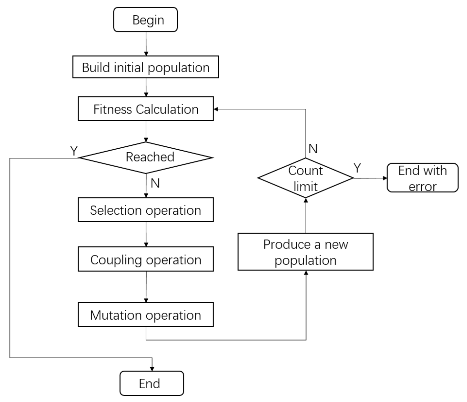
2.4. Solution Procedures

A system simulation program (The original program was developed by Harbin Electric Company Limited, and the Software Copyright Registration Number is 2018SR349409) was developed with the functions energy and exergy balance calculations, parameter sensitivity analyses, and system performance optimizations. Multiobjective optimization was performed using a genetic algorithm developed in Python 3 (Figure 2), which was crosschecked with an enumeration algorithm. A genetic algorithm begins with randomly selected values of parameters (as the initial population). Then, each parameter is evaluated via fitness calculation to test its ability to solve a problem. The selection operation selects some of the parameters for reproduction. The biological crossing over and recombination of parameters are conducted in coupling and mutation operation. Then, a new population is used in a new calculation until the operation objectives are attained.

Table 4. Manipulated parameters in the optimization.

Parameter	Symbol	Range	Step Size
Maximum pressure of the cycle	$p_H$	$\left[15.00, 28.00\right]$ MPa	0.50 MPa
Minimum pressure of the cycle	$p_L$	$\left[8.00, 12.00\right]$ MPa	0.50 MPa
Mass flow rate of the sCO2	${\dot{m}}_{sCO2}$	$\left[300.00, 450.00\right]$ kg/s	1.00 kg/s
Maximum temperature of the cycle	$T_{max}$	$\left[430.00, 480.00\right]$ °C	1.00 °C
Minimum temperature of the cycle	$T_{min}$	$\left[32.00, 38.00\right]$ °C	1.00 °C
Split ratios	r	[0.1, 0.9]	0.05

shows the manipulated parameters in the optimization. The optimization aims to obtain the maximum value of ${\eta }_{exe,cyc}$ or the minimum value of $C_{total}$. The split ratios in the cycle are adjusted based on the optimization process in the range of 0.1–0.9 to obtain the best result. It is one of the optimization parameters, and it is manipulated as other parameters in the genetic algorithm and the enumeration algorithm.

3. Results and Discussions

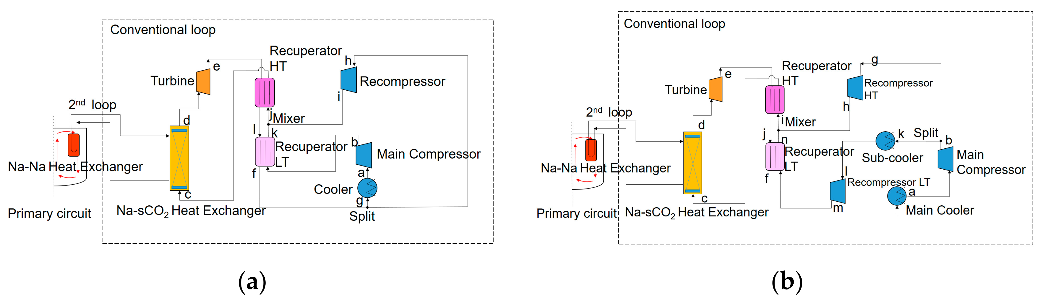
3.1. Energy and Exergy Analyses with Different Layouts

The heat and work distribution of the recuperation cycle based on the energy and exergy analyses in previous studies is shown in Figure 3a. The heat flow map indicates that the heat flow rate into the cycle (${\dot{Q}}_{in}$) was set as the reference quantity of energy. The power input was 0.137${\dot{Q}}_{in}$ when 1${\dot{Q}}_{in}$ energy came into the cycle to support the sCO₂ compression. As the output energy, the turbine output 0.473${\dot{Q}}_{in}$ as power, while the energy released 0.664${\dot{Q}}_{in}$ from the cooler. The heat flow rate of the recuperator in the recuperation process, which is an enormous heat exchange process, was 1.497${\dot{Q}}_{in}$. The cooler wasted a considerable amount of energy according to the heat flow map. However, the discharging energy from the cooler could not be reused due to the low pressure and temperature.

The exergy flow map and the exergy losses of the process to improve the cycle structure are illustrated and shown in Figure 3b. The exergy flow rate into the cycle (${\dot{E}}_{in}$) was set as the reference quantity of exergy in the exergy flow map. The input exergies were 1${\dot{E}}_{in}$ and 0.23${\dot{E}}_{in}$ from the heat source and the compression process, respectively. The main output exergy was 0.81${\dot{E}}_{in}$ via the turbine. Exergy losses mainly occurred in the recuperation, cooling, and heat exchange in the heat source processes as 0.17${\dot{E}}_{in}$, 0.10${\dot{E}}_{in}$, and 0.06${\dot{E}}_{in}$, respectively. Most exergy losses occurred in the heat exchange processes; thus, many types of cascade cycles could be adopted to reduce the exergy losses. Among these cycles, the recompression cycle, which is known as the Feher cycle, had good performance application in the sCO₂ Brayton cycle with the SFR, as shown in Figure 4a. Moreover, the partial cooling in Figure 4b had a relatively simple structure and good performance compared to the compression cycle. The energy and exergy performance of the compression cycle were analyzed in the previous research. The current research focuses on the study of the partial-cooling cycle and completes its comparison with the compression cycle.

3.2. System Performance of the Partial-Cooling Cycle

The optimization of the sCO₂-SFR with the partial-cooling layout at the highest exergy efficiency reaching 63.65% with a net power output of 34.39 MW is shown in Figure 5. A series of parameter limitations was set during the optimization based on the engineering practice, as listed in Table 4.

Figure 6 shows the T-s diagram of the recompression [30] and partial-cooling cycle with optimization results. Compared with the recompression cycle, the compression processes are more complex, including three parts. In the partial-cooling cycle, the pressure of the working fluid was raised in the main compressor (a–b). A part of sCO₂ was cooled in the subcooler (k–l), and the recompressor LT further raised the working fluid pressure (l–m), and then the temperature of sCO₂ was increased in the recuperator LT (m–n). The other part of sCO₂ from the main compressor went into the recompressor HT (g–h) without the cooling process. Both sCO₂ streams entered the mixer with roughly comparable temperatures. sCO₂ went into the recuperator HT to recycle the heat (i–c) after the mixing, and then the working fluid absorbed heat from the heat source of the conventional loop (c–d). Afterward, the working fluid stream with a high temperature and pressure expanded in the turbine (d–e) outputting power. Processes e–j, j–f, and f–a are the heat discharges in the recuperator HT, the recuperator LT, and the main cooler, respectively.

The following observations are presented in

Table 5. Comparisons of exergy losses between the partial-cooling and recompression cycles.

Items	Partial Cooling		Recompression
	Power (MW)	Ratio (%)	Power (MW)	Ratio (%)
${\dot{E}}_{loss,Na-sCO2}$	3.57	6.61	2.06	4.23
${\dot{E}}_{loss,recup}$	5.82	10.77	5.02	10.28
${\dot{E}}_{cooler}$	4.38	8.10	3.17	6.49
${\dot{E}}_{loss,turbine}$	3.60	6.67	3.48	7.13
${\dot{E}}_{loss,comp}$	2.27	4.21	2.37	4.85

: a 3.57 MW exergy loss from the heat source of the conventional loop (6.61%$∆{\dot{E}}_{in}$), a 5.82 MW exergy loss from the recuperators (10.77%$∆{\dot{E}}_{in})$, a 4.38 MW exergy loss from the coolers (8.10%$∆{\dot{E}}_{in})$, a 3.60 MW exergy loss from the turbine (6.67%$∆{\dot{E}}_{in})$, and a 2.27 MW exergy loss from the compressors (4.21%$∆{\dot{E}}_{in})$. Table 5 also reveals that the exergy losses from the Na-sCO₂ heat exchanger were greater in the partial-cooling cycle than in the recompression cycle due to the wide temperature gap between the two sides of the exchanger. Moreover, additional exergy loss was observed from these coolers due to the subcooler application in the partial-cooling cycle.

3.3. Effects of Operation Parameters on Cycle Efficiencies

The cycle efficiencies are discussed on the basis of sensitivity analysis results. The sensitivity of efficiencies to the main system parameters, including the pressure ratio (β = $p_H/p_L$), the inlet temperature of the main compressor ($T_{min}$), and the inlet temperature of the turbine ($T_{max}$), was analyzed.

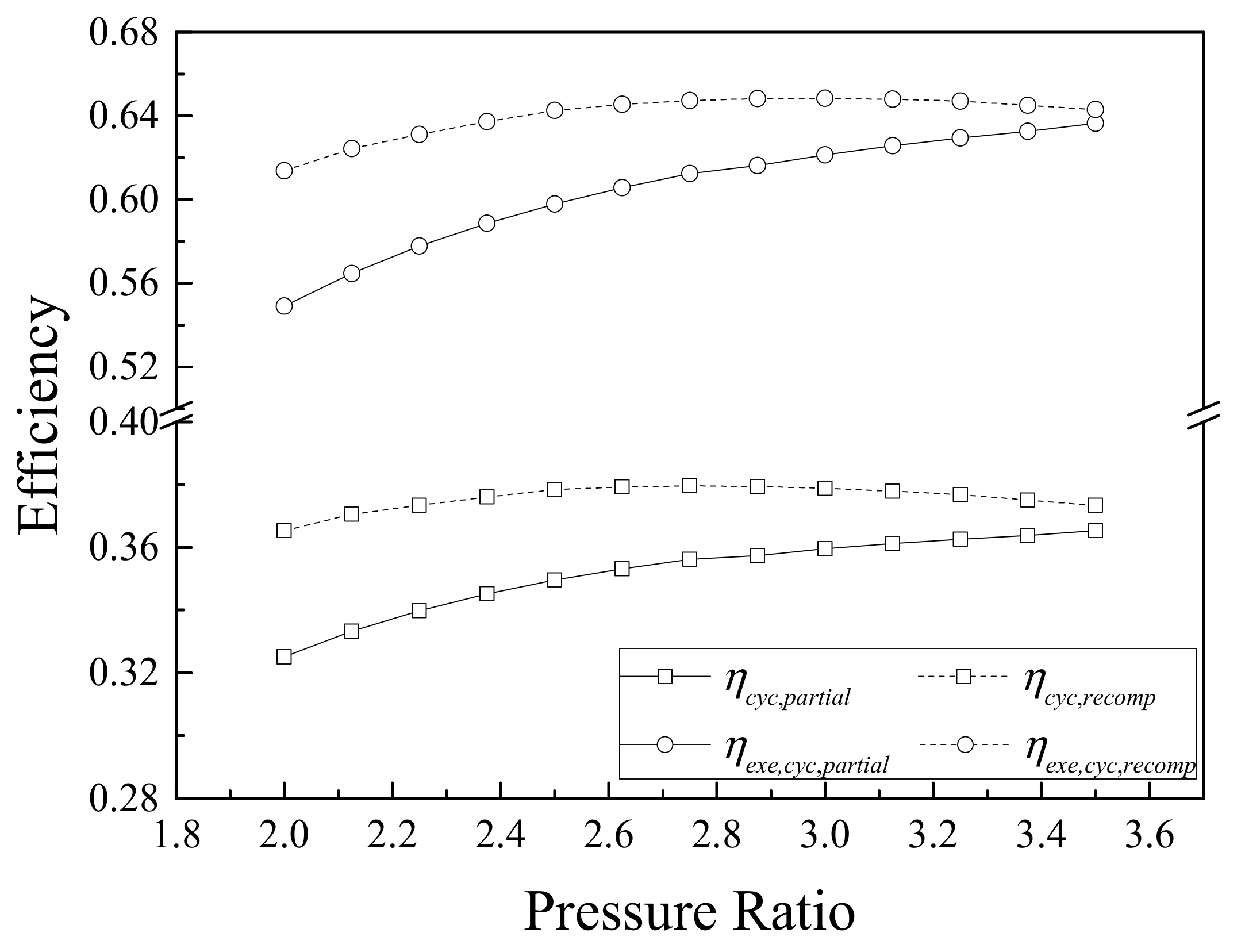
3.3.1. Pressure Ratio

β was set in the range of [2.00, 3.50] with the $p_{comp,in}$ = 8.00 MPa, $T_{min}$ = 35.00 °C, $T_{max}$ = 480.00 °C, and ${\dot{m}}_{C{O}_2}$ = 350.00 kg/s. Theoretically, the maximum β could be reached at a high $p_H$. However, realizing a high $p_H$ is difficult under the current situation of compressor technology. Therefore, only the calculation with the β range in [2.00, 3.50] is shown in this section.

The cycle efficiencies (${\eta }_{cyc}$ and ${\eta }_{exe,cyc}$) of the partial-cooling cycle were generally lower than those of the recompression cycle, as shown in Figure 7, but the gap was narrowed with the increase in β. The effect tendencies of β on ${\eta }_{cyc}$ and ${\eta }_{exe,cyc}$ were based on the partial-cooling cycle rise with the increase in β from 32.51% to 36.53% and from 54.90% to 63.65%, respectively. If the value of β can be raised, then superior system efficiencies could be reached. Unlike the partial-cooling cycle, the maximum value of ${\eta }_{cyc}$ at β = 2.75 was 37.96%, and that of ${\eta }_{exe,cyc}$ at β = 3.00 was 64.84% as observed in the specified β range in the recompression cycle. Therefore, a high β would not elicit a superior system performance in the recompression cycle case.

3.3.2. Inlet Temperature of the Main Compressor

$T_{min}$ cannot be less than 32.00 °C (close to the critical point) because only the supercritical Brayton cycle was considered in this study. The range of $T_{min}$ was decided to fall within [32.00, 36.00] °C with β = 2.75, $p_{comp,in}$ = 8.00 MPa, $T_{max}$ = 480.00 °C, and ${\dot{m}}_{C{O}_2}$ = 428.57 kg/s. Figure 8 shows that the cycle efficiencies of the partial-cooling cycle were better stabilized under $T_{min}$ than the recompression cycle. ${\eta }_{cyc}$ increased initially and decreased from 35.94% to 36.06% (maximum value, at $T_{min}=35.00 °\mathrm{C}$), then to 35.37% under the partial-cooling cycle. Similarly, ${\eta }_{exe,cyc}$ initially rose from 61.68% to 62.31% (maximum value, at $T_{min}=35.00 °\mathrm{C}$) and then dropped to 61.70%. As discussed in Section 3.3.1, the decreasing $T_{min}$ not only reduced the outlet temperature of the compressor, leading to high efficiencies, but also enhanced the heat loss from the subcooler, resulting in energy and exergy losses of steam due to the application of the subcooler. Optimized $T_{min}$, which could maximize the efficiencies, was elicited by the aforementioned influences.

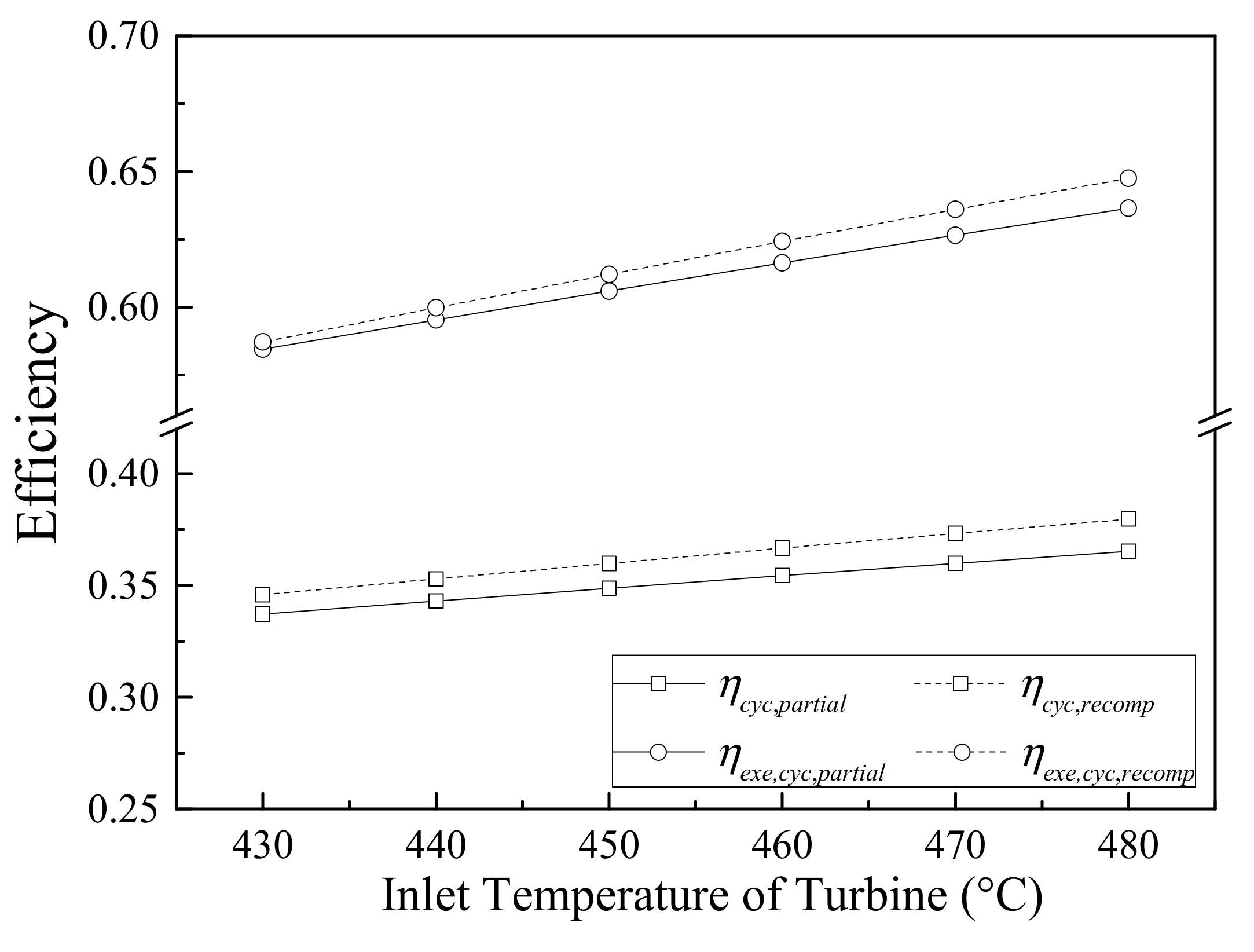
3.3.3. Inlet Temperature of Turbine

Figure 9 shows that the range of $T_{max}$ was decided to fall within [430.00, 480.00] °C with β = 3.5, $p_{comp,in}$ = 8.00 MPa, $T_{min}$ = 35.00 °C, and ${\dot{m}}_{C{O}_2}$ = 350.00 kg/s. ${\eta }_{cyc}$ and ${\eta }_{exe,cyc}$ linearly increased with $T_{max}$ regardless of the partial-cooling or the recompression cycle. ${\eta }_{cyc}$ increased by 2.79% from 33.74% to 36.53% under the partial-cooling cycle, whereas ${\eta }_{exe,cyc}$ dramatically rose by 5.19% from 58.46% to 63.65%. These variations indicate that $T_{max}$ is essential to obtain high ${\eta }_{cyc}$ and ${\eta }_{exe,cyc}$. The highest $T_{max}$ reached in the current research was 480 °C due to the temperature limit of the SFR core (the outlet temperature of the core is close to 550 °C).

The partial-cooling cycle showed a good system performance with the optimization results and the sensitivity analysis. The exergoeconomic of the two layouts will be analyzed in the next section for further comparison.

3.4. Exergoeconomic Discussion

The effects of system parameters on exergoeconomic are initially analyzed in this section. The exergoeconomic optimized results of the partial-cooling cycle are then summarized and compared with the recompression cycle.

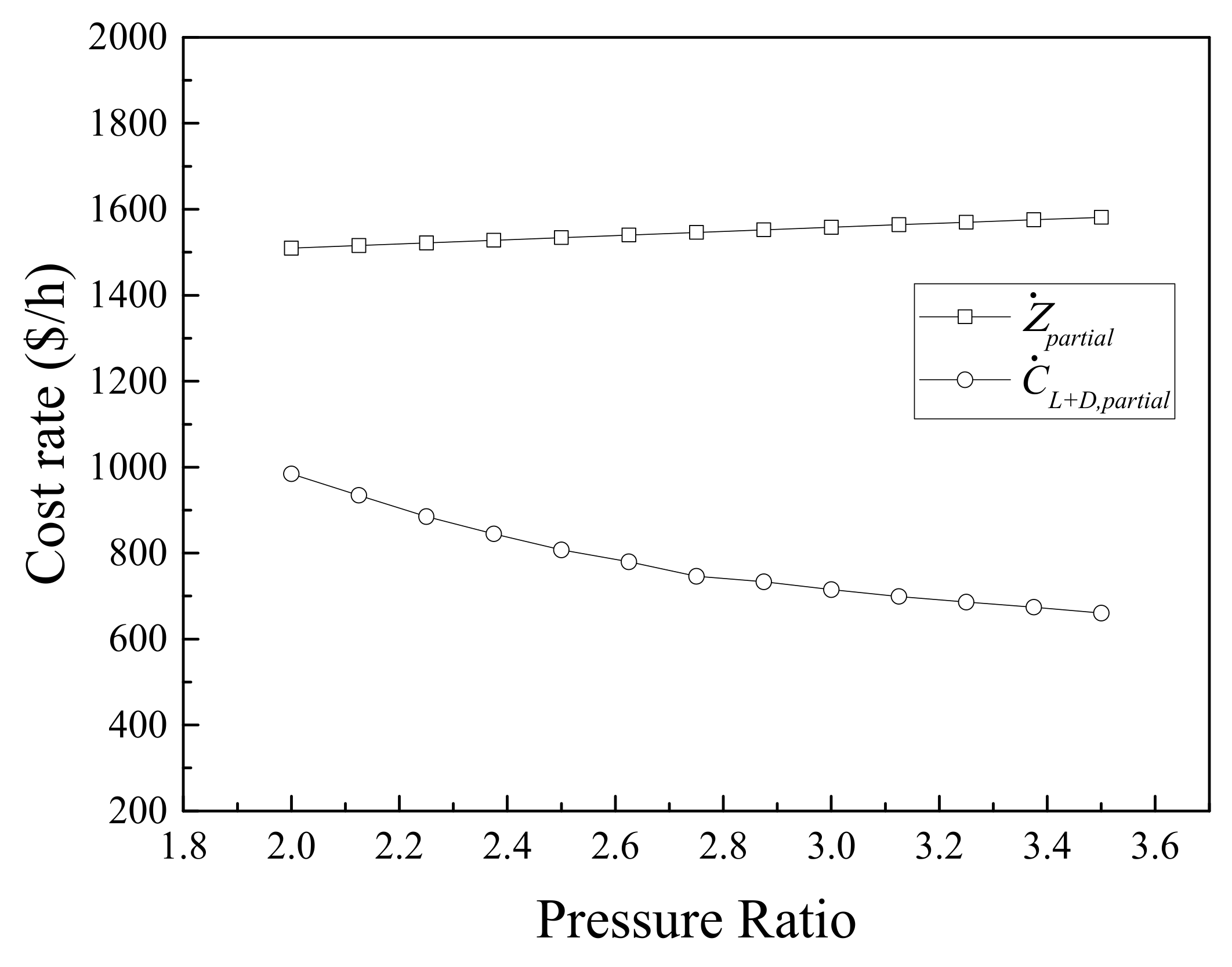
3.4.1. Pressure Ratio

Pressure ratio (β) is a major factor causing cost variation. A large β results in a high outlet pressure of the compressor with the same inlet pressure. Thus, a high outlet pressure would provide additional power support to the compressor. Moreover, the cost of the compressor and the turbine increased in accordance with the equations in Table 1. Figure 10 shows that β was within the range [2.00, 3.50] with $p_{comp,in}$ = 8.00 MPa, $T_{min}$ = 35.00 °C, $T_{max}$ = 480.00 °C, and ${\dot{m}}_{C{O}_2}$ = 428.57 kg/s. ${\dot{C}}_{total}$ dropped 261.19 USD/h from 2491.55 USD/h to 2230.36 USD/h with the partial-cooling cycle. Meanwhile, both efficiencies continuously increased.

${\dot{C}}_{total}$ comprises capital investment, operation, and maintenance costs ($\dot{Z}$), and the cost from exergy loss and destruction (${\dot{C}}_{L+D}$). The effect of β on ${\dot{C}}_{L+D}$ is generally larger than that on $\dot{Z}$, and the variation in ${\dot{C}}_{L+D}$ with β introduces changes in ${\dot{C}}_{total}$. Considering $\dot{Z}$, the increase in β indicates that the maximum cycle pressure would be high, further causing additional $\dot{Z}$ of compressors and turbines. Therefore, $\dot{Z}$ slightly increased with the rise in β, as shown in Figure 11. Unlike $\dot{Z}$, the variation in ${\dot{C}}_{L+D}$ is complicated due to exergy loss and destruction in the partial-cooling cycle, and ${\dot{C}}_{L+D}$ significantly dropped initially and then declined from 984.35 USD/h to 660.20 USD/h.

${\dot{C}}_{component}$ is the total cost of each component, such as the compressor, the cooler, the turbine, the recuperator, and the Na-sCO₂ heat exchanger. As seen in Figure 12, the total cost of the Na-sCO₂ heat exchanger barely changed with β maintaining a value of around 1570–1580 USD/h. The total costs of other components are shown in Figure 12. Turbines and compressors had a lower cost at lower β. By contrast, the total cost of recuperators decreased with increasing β. With higher β, the exergy of the working fluid at the outlet of turbine decreased, as did the energy needed for recuperation. Therefore, the total cost of recuperator was reduced.

3.4.2. Inlet Temperature of the Main Compressor

Considering the effect of $T_{min}$, the range of $T_{min}$ was decided to fall within [32.00, 38.00] °C when β = 3.00, $p_{comp,in}$ = 8.00 MPa, $T_{max}$ = 480.00 °C, and ${\dot{m}}_{C{O}_2}$ = 350.00 kg/s. The ${\dot{C}}_{total}$ of the partial-cooling cycle was significantly higher than that of the recompression cooling cycle. This value decreased from 2308.44 USD/h to 2249.50 USD/h when $T_{min}$ increased from 32.00 °C to 36.00 °C, and then remained around 2250 USD/h with the increase in $T_{min}$, as shown in Figure 13.

Figure 14 shows that the variation in ${\dot{C}}_{total}$ was caused by the change in ${\dot{C}}_{L+D}$, and $\dot{Z}$ barely changed with $T_{min}$. As the inlet of the compressor, $T_{min}$ increased the outlet temperature of the compressor with the same pressure ratio in the range of [32.00, 38.00] °C in the partial-cooling cycle. However, temperatures were not the major influencing factors on $\dot{Z}$ according to the equations in Table 1. By contrast, $T_{min}$ can affect the variations in exergy loss and destruction in the entire system. ${\dot{C}}_{L+D}$ decreased by 60.55 USD/h from 759.31 USD/h to 698.76 USD/h when $T_{min}$ varied from 32.00 °C to 36.00 °C, and then remained at approximately 700 USD/h. ${\dot{C}}_{L+D}$ continued to decrease with the increase in $T_{min}$ when $T_{min}$ was less than 35.00 °C.

Figure 15 shows the variation in component total cost with $T_{min}$. $T_{min}$ hardly affected the total cost of turbines and compressors. The total cost of the Na-sCO₂ heat exchanger barely changed with β maintained around 1564–1584 USD/h. The total cost of the recuperator continued to decrease with the increase in $T_{min}$. During the compression process, a higher outlet temperature of the compressor could be obtained with higher $T_{min}$. The former narrowed the temperature gap of the recuperators. Therefore, the heat exchange capacity and the cost of recuperators were reduced.

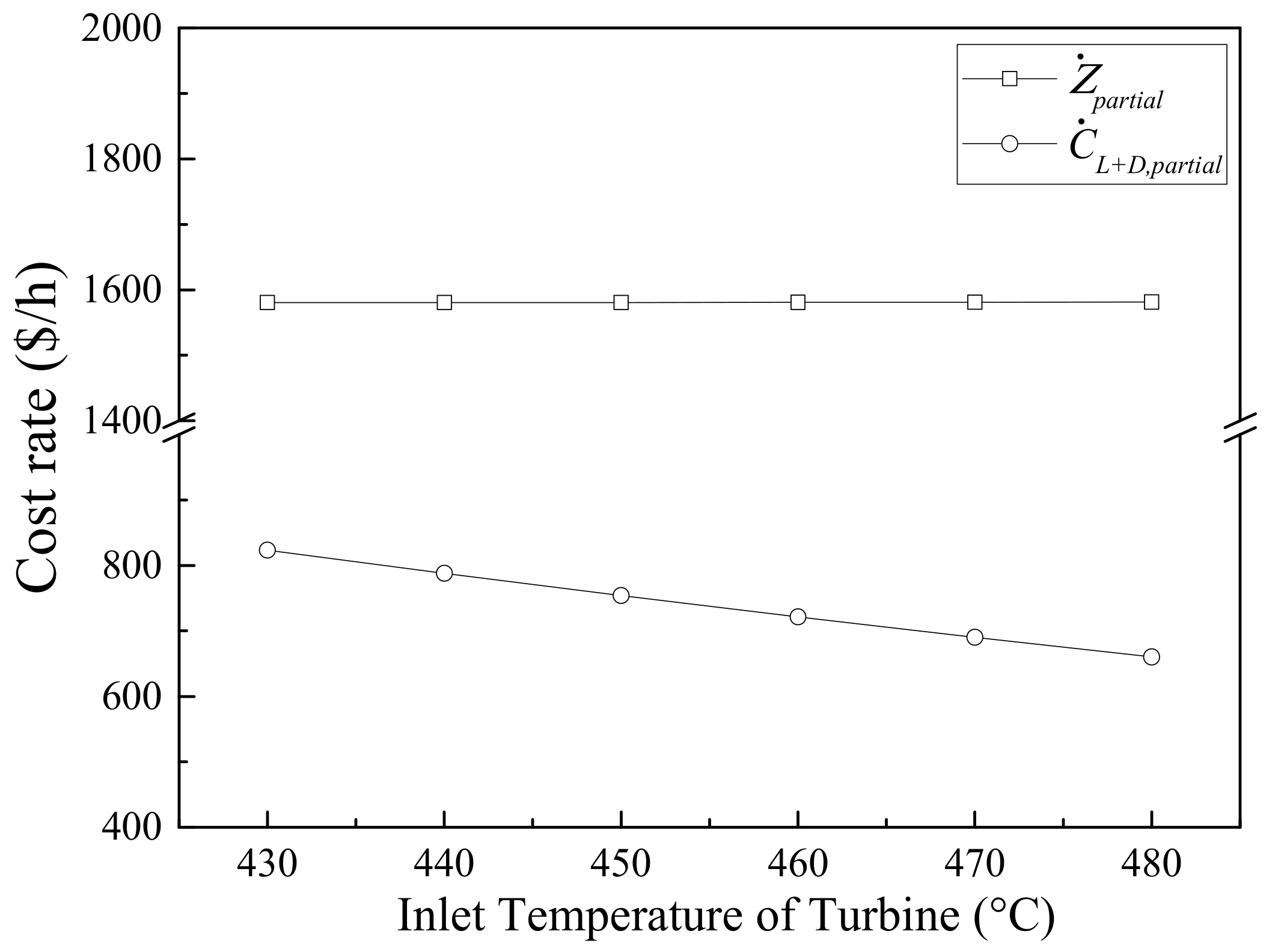
3.4.3. Inlet Temperature of Turbine

Figure 16 shows that the range of $T_{max}$ was decided to fall within [430.00, 480.00] °C when β = 3.50, $p_{comp,in}$ = 8.00 MPa, $T_{min}$ = 35.00 °C, and ${\dot{m}}_{C{O}_2}$ = 350.00 kg/s. The ${\dot{C}}_{total}$ variation lines linearly declined with the increase in $T_{max}$, from 2251.67 USD/h to 2088.88 USD/h (for the recompression cycle) [30] and from 2392.85 USD/h to 2230.36 USD/h (for the partial-cooling cycle). Increasing $T_{max}$ was one of the most effective approaches to reducing the total cost considering system efficiencies. However, the heat source temperature for SFR limited the $T_{max}$ of the sCO₂ cycle. High $T_{max}$ could be reached in the future with the optimization of the SFR core design and the performance enhancements of the Na-sCO₂ heat exchanger.

Similar to the effect of β and $T_{min}$, Figure 17 shows that $\dot{Z}$ barely changed with $T_{max}$. ${\dot{C}}_{L+D}$ dropped because the increase in $T_{max}$ reduced the exergy loss and the destruction of the cycle from 823.42 USD/h to 660.20 USD/h for the partial-cooling cycle.

Figure 18 shows the variation in component total costs with $T_{max}$. $T_{max}$ barely affected the total cost of turbines and compressors. The total cost of the compressor, cooler, turbine, and recuperator barely changed with $T_{max}$. However, the total cost of the Na-sCO₂ heat exchanger was significantly affected by $T_{max}$. The total cost of the recuperator decreased by increasing $T_{max}$; the former dropped about 155.36 USD/h when $T_{max}$ changed from 430 °C to 480 °C.

The comparison among β, $T_{min}$, and $T_{max}$ revealed that the change in ${\dot{C}}_{L+D}$ with β was substantially larger than that with $T_{max}$ or $T_{min}$. Thus, manipulating β is important to guarantee the good economy of the system. Moreover, the sum of capital investment, operation, and maintenance costs ($\dot{Z}$) accounted for large proportions of the total cost rate, which was almost double that of ${\dot{C}}_{L+D}$ in each condition.

3.5. Comparison Summary of the Two Layouts

The partial-cooling cycle showed good system performance with high efficiency and net power via the optimization process based on the operation conditions of the SFR in this study.

Compared with the recompression cycle, the exergy losses from the Na-sCO₂ heat exchanger were greater in the partial-cooling cycle due to the wide temperature gap between the two sides of the exchanger. Moreover, the coolers demonstrated additional exergy losses due to the subcooler application in the partial-cooling cycle.

Furthermore, the recompression cycle could slightly improve the exergoeconomic performance compared to the partial-cooling cycle. The minimum ${\dot{C}}_{total}$ of 2230.36 USD/h with ${\eta }_{exe,cyc}$ = 63.65% could be obtained for the partial-cooling cycle, where β = 3.50, $T_{min}$ = 35.00 °C, and $T_{max}$ = 480.00 °C. Similarly, the minimum ${\dot{C}}_{total}$ reached 2088.88 USD/h with ${\eta }_{exe,cyc}$ = 64.72% at β = 2.75 for the recompression cycle [30]. Meanwhile, the partial-cooling cycle showed good potential for reducing the total cost by increasing the pressure ratio with the development of sCO₂ technology.

4. Conclusions

The current research investigated the system performance and carried out economic analysis of the sCO₂ Brayton cycle for the SFR with a partial-cooling layout. The exergy efficiency of the partial-cooling cycle reached 63.65% with a net power output of 34.39 MW after optimization, and the minimum ${\dot{C}}_{total}$ was 2230.36 USD/h. Similarly, the minimum ${\dot{C}}_{total}$ reached 2088.88 USD/h with ${\eta }_{exe,cyc}$ = 64.72% at β = 2.75 for the recompression cycle. Compared with the recompression cycle, the exergy losses from the Na-sCO₂ heat exchanger were greater in the partial-cooling cycle due to the wide temperature gap between its two sides. Moreover, the coolers had additional exergy losses due to the subcooler application in the partial-cooling cycle.

The cost derived from exergy loss and destruction in the selected ranges of parameters were significantly affected by the pressure ratio and the inlet temperatures of the main compressor and the turbine. The change in cost from exergy loss and destruction with the pressure ratio was substantially greater than that from the inlet temperature of the turbine or the inlet temperature of the main compressor. The total cost of recuperators decreased with the increase in β, $T_{min}$. In addition, the total cost of the recuperator could be reduced by increasing $T_{max}$. Therefore, manipulating β is important to guarantee the good economy of the system. Moreover, the capital investment and operation and maintenance costs normally accounted for large proportions of the total cost rate, which was almost double the cost from exergy loss and destruction in each condition. The partial-cooling cycle obtained the minimum total cost rate when the pressure ratio was equal to 3.50. The inlet temperatures of the main compressor and the turbine were 35 °C and 480 °C, respectively.

References

1. Gianfranco, A. Method for Obtaining Mechanical Energy from a Thermal Gas Cycle with Liquid Phase Compression. U.S. Patent No. 3376706, 9 April 1968. [Google Scholar]
2. Nami, H.; Mahmoudi, S.M.S.; Nemati, A. Exergy, ecomomic and environmental impact assessment and optimization of a novel cogeneration system including a gas turbine, a supercritical CO2 and an organic Rankine cycle (GT-HRSG/SCO2). Appl. Therm. Eng. 2017, 110, 1315–1330. [Google Scholar] [CrossRef]
3. Chaudhary, A.; Mulchand, A.; Dave, P. Feasibility Study of Supercritical CO2 Rankine Cycle for Waste Heat Recovery, Proceedings. In Proceedings of the 6th International Symposium-Supercritical CO2 Power Cycles, Pittsburgh, PA, USA, 27–29 March 2018. [Google Scholar]
4. Xie, M.; Xie, Y.H.; He, Y.C.; Dong, A.H.; Zhang, C.W.; Shi, Y.W.; Zhang, Q.H.; Yang, Q.G. Thermodynamic analysis and system design of the supercritical CO2 Brayton cycle for waste heat recovery of gas turbine. Heat Transf. Res. 2020, 51, 129–146. [Google Scholar] [CrossRef]
5. Siddiqui, M.E. Thermodynamic Performance Improvement of Recopression Brayton Cycle Utilizing CO2-C7H8 Binary Mixture. Mechanika 2021, 27, 259–264. [Google Scholar] [CrossRef]
6. Manzolini, G.; Binotti, M.; Bonalumi, D.; Invernizzi, C.; Iora, P. CO2 mixtures as innovative working fluid in power cycles applied to solar plants. Techno-economic assessment. Sol. Energy 2019, 181, 530–544. [Google Scholar] [CrossRef]
7. Li, H.; Zhang, Y.; Yang, Y.; Han, W.; Yao, M.; Bai, W.; Zhang, L. Preliminary design assessment of supercritical CO2 cycle for commercial scale coal-fired power plants. Appl. Therm. Eng. 2019, 158, 113785. [Google Scholar] [CrossRef]
8. Shi, Y.; Zhong, W.; Shao, Y.; Xiang, J. System Analysis on Supercritical CO2 Power Cycle with Circulating Fluidized Bed Oxy-Coal Combustion. J. Therm. Sci. 2019, 28, 505–518. [Google Scholar] [CrossRef]
9. Siddiqui, M.E.; Almitani, K.H. Proposal and Thermodynamic Assessment of S-CO2 Brayton Cycle Layout for Improved Heat Recovery. Entropy 2020, 22, 305. [Google Scholar] [CrossRef] [Green Version]
10. Haroon, M.; Sheikh, N.A.; Ayub, A.; Tariq, R.; Sher, F.; Beheta, A.T.; Imran, M. Exergetic, Economic and Exergo-Environmental Analysis of Bottoming Power Cycles Operating with CO2-Based Binary Mixture. Energies 2020, 13, 5080. [Google Scholar] [CrossRef]
11. Garg, P.; Srinivasan, K.; Dutta, P.; Kumar, P. Comparison of CO2, and Steam in Transcritical Rankine Cycles for Concentrated Solar Power. Energy Procedia 2014, 49, 1138–1146. [Google Scholar] [CrossRef] [Green Version]
12. Dunima, S.; Jahn, I.; Hooman, K.; Lu, Y.; Veeraragavan, A. Comparison of direct and indirect natural draft dry cooling tower cooling of the sCO2 Brayton cycle for concentrated solar power plants. Appl. Therm. Eng. 2018, 130, 1070–1080. [Google Scholar] [CrossRef]
13. Handwerk, C.S.; Driscoll, M.J.; Hejzlar, P. Optimized Core Design of a Supercritical Carbon Dioxide-Cooled Fast Reactor. Nucl. Technol. 2007, 164, 3320–3336. [Google Scholar] [CrossRef]
14. Pope, M.A. Thermal hydraulic design of a 2400 MWth Direct Supercritical Co-Cooled Fast Reactor. Ph.D. Thesis, Institute of Technology, Cambridge, MA, USA, 2006. [Google Scholar]
15. Gao, W.; Yao, M.Y.; Chen, Y.; Li, H.; Zhang, Y.; Zhang, L. Performance of S-CO2 Brayton Cycle and Organic Rankine Cycle (ORC) Combined System Considering the Diurnal Distribution of Solar Radiation. J. Therm. Sci. 2019, 28, 463–471. [Google Scholar] [CrossRef]
16. Nuclear Development Report, Risks and Benefits of Nuclear Energy; NEA No. 6242; OECD Nuclear Energy Agency: Paris, France, 2007.
17. Sienicki, J.J.; Moisseytsev, A. Nuclear Power. In Fundamentals and Applications of Supercritical Carbon Dioxide (sCO2) Based Power Cycles; Brun, K., Friedman, P., Dennis, R., Eds.; Woodhead Publishing: Sawston, UK, 2017; pp. 339–391. [Google Scholar]
18. Hoffmann, J.R.; Feher, E.G. 150 kWe Supercritical Closed Cycle System. ASME J. Eng. Power. 1971, 93, 70–80. [Google Scholar] [CrossRef]
19. Feher, E.G.; Harvey, R.A.; Milligan, H.H. 150-kWe Supercritical Cycle Turbo-pump Design Layout and Performance Demonstration Final Technical Report; McDonnell Douglas Astronautics Company-West: St. Louis, MO, USA, 1971. [Google Scholar]
20. Dievoet, V.J.P. The sodium-CO2 fast breeder reactor concept. In Proceedings of the International Conference on Sodium Technology and Large Fast Reactor Design, Bologna, Italy, 7–9 November 1968. [Google Scholar]
21. Sienicki, J.J.; Moisseytsev, A.; Krajtl, L. A Supercritical CO2 Brayton Cycle Power Converter for a Sodium-Cooled Fast Reactor Small Modular Reactor. In Proceedings of the ASME 2015 Nuclear Forum collocated with the ASME 2015 Power Conference, the ASME 2015 9th International Conference on Energy Sustainability, and the ASME 2015 13th International Conference on Fuel Cell Science, Engineering and Technology. American Society of Mechanical Engineers, San Diego, CA, USA, 28 June–2 July 2015. V001T01A004. [Google Scholar]
22. Grandy, C.; Sienicki, J.J.; Moisseytsev, A.; Krajtl, L.; Farmer, M.T.; Kim, T.K.; Middleton, B. Advanced Fast Reactor—100 (AFR-100) Report for the Technical Review Panel; U.S. Department of Commerce National Technical Information Service: Alexandra, VA, USA, 2014. [Google Scholar]
23. Masakazu, I.; Tomoyasu, M.; Shoji, K. A Next Generation Sodium-cooled Fast Reactor Concept and Its R&D Program. Nucl. Eng. Technol. 2007, 3, 171–186. [Google Scholar]
24. Moisseytsev, A.; Sienicki, J.J. Investigation of alternative layouts for the supercritical carbon dioxide Brayton cycle for a sodium-cooled fast reactor. Nucl. Eng. Des. 2009, 239, 1362–1371. [Google Scholar] [CrossRef]
25. Xie, M.; Xie, Y.H.; Zhang, Q.H.; He, Y.; Dong, A.; Zhang, C.; Shi, Y.; Yang, Q. Thermodynamic Analysis and Multiple System Layouts Comparison of the Supercritical CO2 Brayton Cycle for Sodium-cooled Fast Reactor with Offshore Scenes. In Proceedings of the International Conference on Energy, Ecology and Environment (ICEEE 2018) and International Conference on Electric and Intelligent Vehicles (ICEIV 2018), Melbourne, Australia, 21–25 November 2018. [Google Scholar]
26. Neises, T.; Turchi, C. Supercritical CO2 Power Cycles: Design Considerations for Concentrating Solar Power. In Proceedings of the The 4th International Symposium-Supercritical CO2 Power Cycles, Pittsburgh, PA, USA, 9–10 September 2014. [Google Scholar]
27. Lu, S.P.; Liu, Y.W.; Lin, Y.S. Parameters optimization of supercritical carbon dioxide Brayton cycle based on CEFR. Energy Conserv. 2018, 7, 21–26. [Google Scholar]
28. Siddiqui, M.E.; Almitani, K.H. Energy and Exergy Assessment of S-CO2 Brayton Cycle Coupled with a Solar Tower System. Processes 2020, 8, 1264. [Google Scholar] [CrossRef]
29. Noaman, M.; Saade, G.; Morosuk, T.; Tsataronis, G. Exergoeconomic Analysis Applied to Supercrtical CO2 Power Systems. Energy 2019, 183, 756–765. [Google Scholar] [CrossRef]
30. Xie, M.; Xie, Y.; Zhang, Q.; Zhang, C.; Dong, A.; Shi, Y.; Zhang, Y. Exergy and Exergoeconomic Analyses Based on Recompression Cycle of the Supercritical CO2 Brayton Cycle for Sodium-cooled Fast Reactor. In Proceedings of the International Conference on Energy, Ecology and Environment (ICEEE 2019) and International Conference on Electric and Intelligent Vehicles (ICEIV 2019), Stavanger, Norway, 23–27 July 2019. [Google Scholar]
31. Shokati, N.; Mohammadkhani, F.; Yari, M.; Mahmoudi, S.M.S.; Rosen, M.A. A comparative exergoeconomic analysis of waste heat recovery from a gas turbine-modular helium reactor via organic Rankine cycles. Sustainability 2013, 6, 2474–2489. [Google Scholar] [CrossRef] [Green Version]
32. Mohammadkhani, F.; Shokati, N.; Mahmoudi, S.M.S.; Yari, M.; Rosen, M.A. Exergoeconomic assessment and parametric study of a gas turbine-modular helium reactor combined with two organic rankine cycles. Energy 2014, 65, 533–543. [Google Scholar] [CrossRef]
33. Khaljani, M.; Saray, R.K.; Bahlouli, K. Comprehensive analysis of energy, exergy and exergo-economic of cogeneration of heat and power in a combined gas turbine and organic rankine cycle. Energy Convers. Manag. 2015, 97, 154–165. [Google Scholar] [CrossRef]
34. Schultz, K.R.; Brown, L.C.; Besenbruch, G.E.; Hamilton, C.J. Large Scale Production of Hydrogen by Nuclear Energy for the Hydrogen Economy; GA-A24265; General Atomics: San Diego, CA, USA, 2003. [Google Scholar]
35. Ghaebi, H.; Amidpour, M.; Karimkashi, S.; Rezayan, O. Energy, exergy and thermoeconomic analysis of a combined cooling, heating and power (CCHP) system with gas turbine prime mover. Int. J. Energy Res. 2011, 35, 697–709. [Google Scholar] [CrossRef]
36. Guo, Y.Z.; En, W.; Shan, T.T. Techno-economic study on compact heat exchangers. Int. J. Energy Res. 2008, 32, 1119–1127. [Google Scholar]
37. Dixon, B.; Ganda, F.; Hoffman, E.A.; Hansen, J. Advanced Fuel Cycle Cost Basis—2017 Edition; U.S. Department of Energy Fuel Cycle Options Campaign: Washington, DC, USA, 2017. [Google Scholar]
38. Wang, X.; Yang, Y.; Zheng, Y.; Dai, Y. Exergy and exergoeconomic analyses of a supercritical CO2 cycle for a cogeneration application. Energy 2017, 119, 971–982. [Google Scholar] [CrossRef]
39. Zare, V.; Mahmoudi, S.M.S.; Yari, M. An exergoeconomic investigation of waste heat recovery from the Gas Turbine-Modular Helium Reactor (GT-MHR) employing an ammonia–water power/cooling cycle. Energy 2013, 61, 397–409. [Google Scholar] [CrossRef]
Figure 1. Layouts of the SFR-sCO2 recuperation cycle. a–h represent state points of working fluid in the cycle.
Energies 15 03555 g001
Figure 2. Flow diagram of genetic algorithm method.
Energies 15 03555 g002
Figure 3. Energy and exergy distributions of the recuperation cycle [25]. (a) Heat and power, (b) Exergy and exergy loss. A–h represent state points of working fluid in the cycle.
Energies 15 03555 g003
Figure 4. Advanced cycle layouts of sCO2-SFR. (a) Recompression cycle, (b) partial cooling cycle. a–n represent state points of working fluid in the cycle.
Energies 15 03555 g004
Figure 5. Optimal simulation results of the partial-cooling cycle with sCO2-SFR. a–n represent state points of working fluid in the cycle.
Energies 15 03555 g005
Figure 6. T-s diagram at the optimum point with the advanced cycles. (a) Recompression cycle, (b) partial cooling cycle. a–n represent state points of working fluid in the cycle.
Energies 15 03555 g006
Figure 7. Effects of β on η c y c and η e x e , c y c with the partial-cooling cycle compared with the recompression cycle.
Energies 15 03555 g007
Figure 8. Effects of T m i n on η c y c and η e x e , c y c with the partial-cooling cycle compared with the recompression cycle.
Energies 15 03555 g008
Figure 9. Effects of T m a x on η c y c and η e x e , c y c with the partial-cooling cycle compared with the recompression cycle.
Energies 15 03555 g009
Figure 10. Effects of β on C ˙ t o t a l with the partial-cooling cycle compared with the recompression cycle.
Energies 15 03555 g010
Figure 11. Effects of β on Z ˙ and C ˙ L + D with the partial-cooling cycle.
Energies 15 03555 g011
Figure 12. Effects of β on C ˙ c o m p o n e n t with the partial-cooling cycle.
Energies 15 03555 g012
Figure 13. Effects of T m i n on C ˙ t o t a l with the partial-cooling cycle compared with the recompression cycle.
Energies 15 03555 g013
Figure 14. Effects of T m i n on Z ˙ and C ˙ L + D with the partial-cooling cycle.
Energies 15 03555 g014
Figure 15. Effects of T m i n on C ˙ c o m p o n e n t with the partial-cooling cycle.
Energies 15 03555 g015
Figure 16. Effects of T m a x on η c y c , η e x e , c y c , and C ˙ t o t a l with the partial-cooling cycle compared with the recompression cycle.
Energies 15 03555 g016
Figure 17. Effects of T m a x on Z ˙ and C ˙ L + D with the partial-cooling cycle.
Energies 15 03555 g017
Figure 18. Effects of T m a x on C ˙ c o m p o n e n t with the partial-cooling cycle. (a) Multiple components, (b) Na-sCO2 heat exchanger.
Energies 15 03555 g018