A Real-Time Load Prediction Control for Fuel Cell Hybrid Vehicle

Abstract

The development of hydrogen energy is an effective solution to the energy and environmental crisis. Hydrogen fuel cells and energy storage cells as hybrid power have broad application prospects in the field of vehicle power. Energy management strategies are key technologies for fuel cell hybrid systems. The traditional optimization strategy is generally based on optimization under the global operating conditions. The purpose of this project is to develop a power allocation optimization method based on real-time load forecasting for fuel cell/lithium battery hybrid electric vehicles, which does not depend on specific working conditions or causal control methods. This paper presents an energy-management algorithm based on real-time load forecasting using GRU neural networks to predict load requirements in the short time domain, and then the local optimization problem for each predictive domain is solved using a method based on Pontryagin’s minimum principle (PMP). The algorithm adopts the idea of model prediction control (MPC) to transform the global optimization problem into a series of local optimization problems. The simulation results show that the proposed strategy can achieve a good fuel-saving control effect. Compared with the rule-based strategy and equivalent hydrogen consumption strategy (ECMS), the fuel consumption is lower under two typical urban conditions. In the 1800 s driving cycle, under WTCL conditions, the fuel consumption under the MPC-PMP strategy is 22.4% lower than that based on the ECMS strategy, and 10.3% lower than the rules-based strategy. Under CTLT conditions, the fuel consumption of the MPC-PMP strategy is 13.12% lower than that of the rule-based strategy, and 3.01% lower than the ECMS strategy.

1. Introduction

With the current environmental deterioration and energy crisis, developing clean energy has become an inevitable choice for human sustainable development. Many countries and companies have conducted extensive research and development dedicated to the creation of new alternative and renewable energy sources and technologies. Among these, hydrogen energy is considered to be the most promising green and clean alternative energy for the future. Compared with other alternative energy sources, it has the advantages of low environmental pollution and high efficiency [1].

The proton exchange membrane fuel cell (PEMFC) has become an ideal power source due to its zero emission, high power density, and fast start-up speed, which has attracted extensive attention and has become a research hotspot in various countries. To date, PEMFC has been successfully applied in various operations such as stationary power generation and vehicle power supply. As a vehicle power source in particular, PEMFC has shown great potential and is considered to be an important direction for the sustainable development of the automotive industry in the future.

The vehicle fuel cell hybrid power system is generally composed of a fuel cell system, energy storage device, power electronic converter, and energy management system. Among them, the energy management strategy is one of the key technologies of the hybrid system, which determines the performance of the system. Generally, it can be divided into two types: rule-based and optimization-based.

The rule-based energy management strategy is to allocate energy according to the working characteristics of each subsystem and engineering experience, mainly including deterministic rules and fuzzy logic control. The optimization-based energy management strategy takes the system energy consumption or life durability as the optimization objective for optimal control. It can be divided into two categories: global optimization algorithms such as dynamic programming (DP), and convex optimization and instantaneous optimization algorithms such as equivalent consumption minimization strategy (ECMS) and Pontryagin’s minimum principle (PMP).

Zhou et al. [2] used the adaptive online learning Markov method to predict the future vehicle speed, and designed the reference Stata of Charge (SOC) to implement predictive control according to the prediction results. Liu et al. [3] used nonlinear autoregressive neural networks (NARANN) and performed a dynamic programming moving window method to iteratively update the prediction model, which could provide stable demand power prediction for complex and changeable driving environments. Nie et al. [4] used model predictive control (MPC) based on the fast projection gradient method to comprehensively predict vehicle speed and real-time vehicle conditions, as well as road slope and resistance, to achieve fast and real-time speed sequence planning, but the real-time vehicle conditions need the support of the Internet of vehicles.

Li, X.F [5] adopts a model prediction algorithm to perform instantaneous predictive control for torque distribution or power demand according to driver’s intention. Although real-time optimization can be achieved, its control effect is based on the selection of the initial state and cannot achieve global optimization. Zhou [6] proposes a multi-mode energy management strategy for fuel cell hybrid vehicles. It consists of a Markov driving pattern recognizer and a multimodal MPC controller. The Markov recognizer classifies driving segments measured in real time into one of three predefined patterns and the MPC control parameters are selected and adjusted offline according to the pattern recognition results. In the next layer, local optimization is performed based on the selected control parameters and velocity predictions.

Xu, L, et al. [7] establishes an equivalent fuel consumption model of a fuel cell hybrid vehicle, seeking the lowest instantaneous equivalent fuel consumption of the system. Ref. [8] proposes a state machine control strategy based on droop control, which improves the operational reliability of the fuel cell hybrid tram. Hemi [9] proposes an energy optimization strategy based on Markov chain and PMP. First, the Markov probability transition model is used to predict the load demand, and then the PMP algorithm is used to solve the problem of minimum equivalent hydrogen consumption.

The previous energy management strategies are generally based on optimization under the global operating conditions. However, the vehicle driving conditions under actual road conditions are uncertain and time-varying, so it is generally impossible to obtain the global operating conditions information in advance. If the velocity or power demand information of the next time period can be predicted in advance, it is of great significance for the system energy management system to optimize power allocation, and obtain better control effects. Therefore, this study develops a predictive control based on neural networks to predict the power demand for a period of time in the future, and then carry out global optimization in the prediction domain. Rolling prediction and optimization control will be used to achieve close to the global optimization. For the prediction model, the GRU neural network, which has the advantages of the LSTM neural network, but with a simpler structure, is selected for vehicle speed prediction. Then, Pontryagin’s minimum principle (PMP) method is utilized to optimize in the prediction domain.

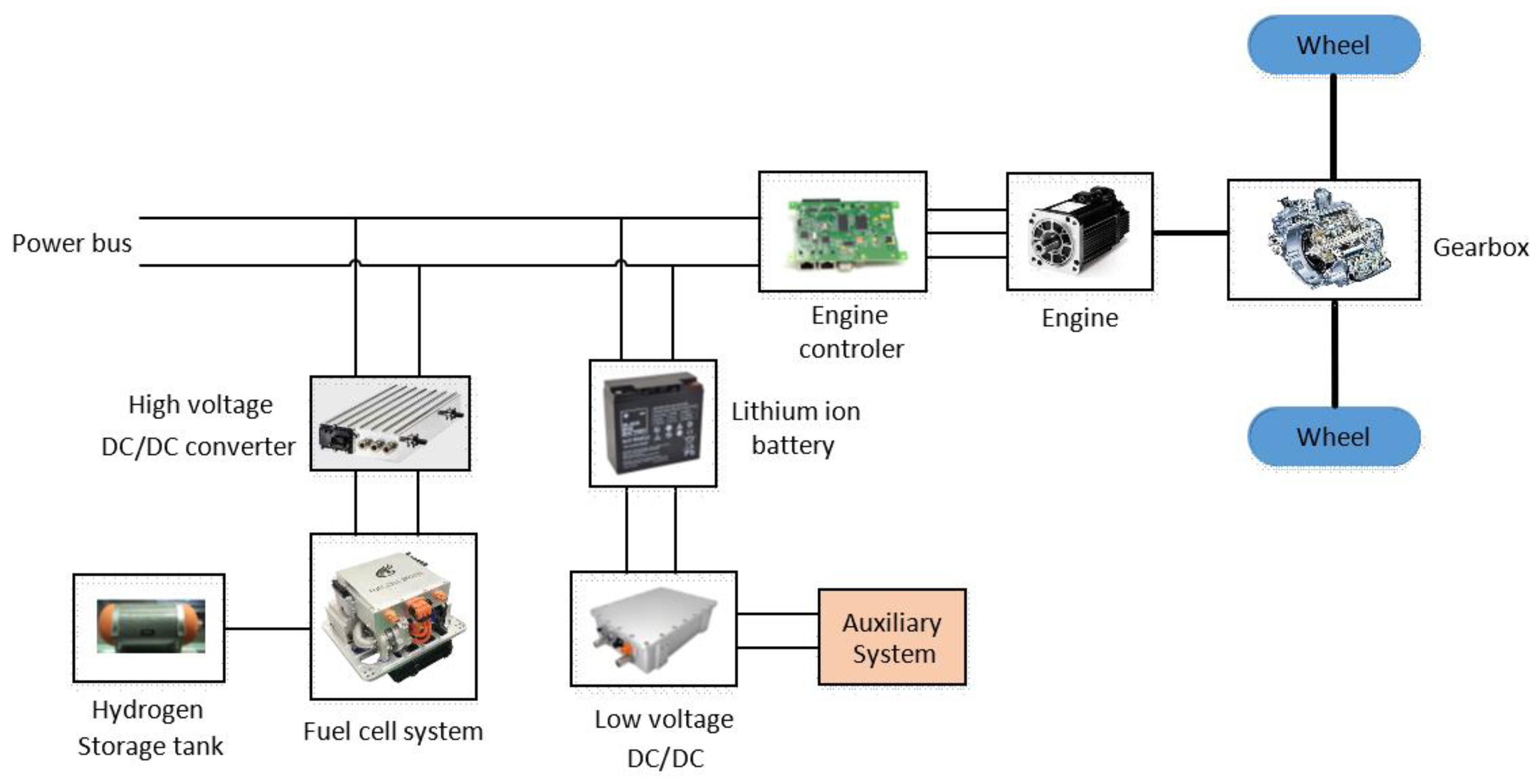
The main research content of this paper includes system modeling and the energy management strategy of a fuel cell hybrid system. The system structure of the fuel cell hybrid system comprises a hydrogen power generation system, battery pack, DC load (electric vehicle, etc.) and corresponding power electronic equipment. The simulation model of each device is established, and the working characteristics of each part are analyzed.

For the hybrid system, it is necessary to consider how to distribute the output power of the energy source to enable the vehicle to run stably and achieve economic and durability targets. The energy management strategy (EMS) controls the output power of the energy source in real time according to the current state of the system, and its control effect directly affects the overall performance of the hybrid system.

2. Vehicle Fuel Cell Powertrain System Model

2.1. Powertrain Description

The hybrid system consists of a proton exchange membrane fuel cell system, an energy storage battery pack, and a corresponding DC/DC conversion module. The fuel cell system is the main power source of a hybrid electric vehicle, and its electrical energy is transmitted to the DC bus through unidirectional DC/DC. The DC/DC converter regulates the current flow from the fuel cell to the DC bus. As an auxiliary power unit, the lithium battery pack is directly connected to the DC bus. When the fuel cell cannot meet the load power demand, the energy storage battery is used as an auxiliary energy source to compensate the energy of the system. During the vehicle’s regenerative braking, the power battery recovers excess energy according to its own conditions to improve energy utilization efficiency. The load is a brushless DC motor, which receives energy from the DC bus and drives the vehicle forward. The powertrain model of the series HEV is shown in Figure 1.

This paper takes a typical urban medium-sized hybrid electric passenger car as the research object. The powertrain can operate in four basic working modes: fuel cell driving mode, lithium battery driving mode, hybrid mode, and regenerative braking mode. The EMS embedded in the onboard VCU guides the energy flow of the powertrain. In order to study the energy management strategy of the FHEV, mathematical models of the powertrain need to be established. The vehicle parameters are shown in

Table 1. Vehicle and powertrain parameters.

Category	Item	Value
Vehicle parameters	Vehicle total mass (kg)	1577
	Wheel radius (m)	0.31
	Aerodynamic drag coefficient (Cd)	0.33
	Vehicle frontal area (m2)	2.254
	Air density (kg/m3)	1.21
	Rolling coefficient	0.013
	Drive efficiency	0.945
PEMFC system Lithium-ion battery pack Electric motor	Rated power (kW)	40
	Capacity (Ah)	20
	Open circuit voltage (V)	350
	Rated power (kW)	75

.

2.2. Fuel Cell System

The fuel cell system is the primary energy source of the system, including the fuel cell stack and the auxiliary system. In this study, we use a voltage model, power model, and hydrogen consumption model to describe the external characteristics of the vehicle fuel cell system.

2.2.1. Voltage Model

The actual output voltage of the fuel cell can be represented by the thermodynamically predicted voltage and subtracting various overvoltage losses. The voltage model of a single cell is as follows [8]:

$$v_{fc}=E-v_{act}-v_{ohm}-v_{conc}$$

(1)

Here, E is the theoretical open circuit voltage.$v_{act}$, $v_{ohm}$, and $v_{conc}$ represent activation loss, ohmic loss, and concentration loss, respectively.

2.2.2. Power Model

As the core of the PEMFC system, the fuel cell stack converts hydrogen energy into electricity through electrochemical reactions. The power $P_{\mathrm{stack} }$ provided by the stack is related to the stack current $I_{\mathrm{stack} }$ and the cell voltage $v_{fc}$ as follows:

$$P_{\mathrm{stack} }=N_{\mathrm{cell} }\cdot v_{fc}\cdot I_{\mathrm{stack} }$$

(2)

Here, $N_{\mathrm{cell} }$ represents the number of cells in the stack.

A small part of the electrical energy ($P_{\mathrm{aux} }$) generated by the stack is used for auxiliary systems, such as air compressors, to ensure the normal operation of the entire system. The part of the power used to drive the vehicle is called net power. The actual output (net) power of the PEMFC system is equal to the difference between $P_{\mathrm{stack} }$ and $P_{\mathrm{aux} }$:

$$P_{\mathrm{fc}}=P_{\mathrm{stack} }-P_{\mathrm{aux} }$$

(3)

2.2.3. Hydrogen Consumption Model

During the operation of the PEMFC, the hydrogen mass consumption can be calculated as follows [10]:

$${ \mathrm{M}}_{{\mathrm{H}}_2}={\int }_0^t\frac{P_{\mathrm{FC}}\left(\tau \right)}{{\eta }_{\mathrm{FCS}}·{\mathrm{LHV}}_{{\mathrm{H}}_2}}\mathrm{d}\tau$$

(4)

Among them, ${\eta }_{\mathrm{FCS}}$ is the efficiency of the PEMFC system, and ${\mathrm{LHV}}_{{\mathrm{H}}_2}$ is the low-heating value (LHV) of ${\mathrm{H}}_2$ (120 kJ/g).

2.3. Battery System

In this paper, a power battery is used as the auxiliary energy source of the hybrid system. A lithium-ion battery with high specific energy and specific power performance is adopted. The main parameters of the single lithium-ion battery are shown in

Table 2. Parameters of Li-ion battery unit.

Parameter	Value
Rated voltage/V	3.2
Rated capacity/Ah	20
Internal resistance/$\mathrm{m}\mathsf{\Omega }$	≤10
Operating temperature/°C	−20~45

.

The battery is used to respond to the power demands during rapid load changes or heavy loads, and to recover excess energy during braking.

The battery model is a simplification and description of the external characteristics of the battery, and is an essential part of the HEV simulation.

For lithium-ion batteries, this study selects the internal resistance equivalent circuit model, which has fewer parameters. Figure 2 shows a typical battery internal resistance model where $R_{int}$ represents internal resistance and $V_{oc}$ is the open circuit voltage.

The vehicle control needs to consider the battery charging and discharging, which is a complex electrochemical process, accompanied by temperature changes and electrochemical reactions. The usual treatment is to equate the open circuit voltage and internal resistance as a function of $SOC$ and temperature [8]. In this study, it is assumed that the battery circuit parameters do not change with temperature.

According to the equivalent circuit, the DC bus voltage of a single battery can be expressed as:

$$V_{bat}=V_{oc}\left(SOC,T\right)-I_{bat}\cdot R_{int}\left(SOC,T\right)$$

(5)

Here, $I_{bat}$ is the battery current in equivalent circuit, and $R_{int}$ refers to the equivalent internal resistance of the battery, which can be divided into discharge resistance and charging resistance.

Assuming that the battery temperature is constant,

$$V_{bat}=V_{oc}\left(SOC\right)-I_{bat}\cdot R_{int}\left(SOC\right)$$

(6)

where $V_{\mathrm{oc} }$ is the open circuit voltage of the battery.

This characteristic can be found in the data sheet of the studied battery, or obtained from experimental tests [11]. Figure 3 shows the open circuit voltage and internal resistance as a function of $SOC$, where $R_{dis}$ represents the discharge resistance of battery and $R_{ch}$ represents the charge resistance of the battery.

Assuming that the battery temperature is constant and considering the internal electrical loss, the battery output power:

$$P_{bat}\left(t\right)=P_b-P_l=V_{oc}{I}_{bat}\left(t\right)-I_{bat}^2\left(t\right)R_{int}$$

(7)

where $P_{bat}$ is the total power of the input or output battery, $P_b$ is the power at the terminal, $P_l$ is the internal friction of the battery, and $I_{bat}$ and $R_{int}$ is the terminal current and equivalent internal resistance of the battery, respectively.

The battery current can be obtained by solving Equation (7):

$$I_{bat}\left(t\right)=\frac{V_{OC}-\sqrt{V_{OC}^2-4R_{int}·P_{bat}\left(t\right)}}{2R_{int}}$$

(8)

where $R_{int}$ is the internal resistance, and $V_{OC}$ and $R_{int}$ are the functions of the battery SOC.

SOC is defined as the percentage of the remaining capacity of the battery relative to the nominal capacity. The $SOC$ of the battery can be described as:

$$SOC\left(t\right)=SO{C}_0-{\int }_0^t\frac{{\eta }_{bat}\cdot I_{bat}\left(\tau \right)}{Q_{bat}}\mathrm{d}\tau ,SOC\in \left[0,1\right]$$

(9)

where $SO{C}_0$ is the initial SOC and ${\eta }_{\mathrm{BAT}}$ is the battery efficiency. $Q_{bat}$ is the nominal capacity (Ah) of the battery, and $I_{bat}$ is the current of the battery. The change rate of SOC is defined as the ratio of terminal current to battery capacity [12].

2.4. DC/DC System

The buck-boost DC converter is used to convert the fuel cell output voltage to the required DC bus voltage. Ignoring the transient response of the buck-boost converter, the static model of the buck-boost converter can be established [13]:

$$\eta \left(k\right)V_{\mathrm{fc}}\left(k\right)I_{\mathrm{fc}}\left(k\right)=V_B\left(k\right)I_{\mathrm{dc}}\left(k\right)$$

(10)

where $\eta$ represents the power transfer efficiency of the buck-boost converter, which varies with the input power, $V_B$ represents the bus voltage, and $I_{\mathrm{dc}}$ represents the output current of DC power supply.

3. Energy Management Strategy

Fuel cell hybrid vehicles typically adopt a rule-based or optimized distribution strategy. The rule-based strategy is causal, but it does not guarantee the optimality of the control effect. Conversely, optimization-based solutions usually ensure optimal power distribution through mathematical optimization; however, they lead to a lack of causality and are difficult to implement online. Therefore, a challenge lies in how to develop an appropriate energy management strategy to seek a balance between optimal and real-time performance [14].

In a sense, model predictive control (MPC) can be regarded as a compromise between instantaneous optimization and global optimization. The MPC algorithm estimates the upcoming power requirements in a finite time range and solves the optimal power allocation decision at each receding horizon. It can effectively reduce the amount of computation. Through rolling optimization, the actual control effect is close to the global optimal [15].

This study adopts the idea of MPC by transforming the global optimal control problem of the whole driving cycle into a local optimal problem in the prediction domain, and then updating the next time domain by constantly rolling the optimization.

3.1. Model Predictive Control

The process of MPC energy management can be divided into three steps: state prediction, objective function solution, and optimal control action application. The model predictive control energy management strategy for optimal fuel economy is shown in Figure 4.

By transforming the global optimization into a series of sub-optimizations, MPC can obtain the optimal local control law. A typical MPC-based energy management strategy consists of three steps [11].

(1)

State prediction

The prediction model is established, the vehicle speed is selected as the prediction quantity, and the future speed is predicted in the finite time domain $t_k\sim t_k+H_p$ at each sampling time. The driving demand power in the prediction domain is calculated.

(2)

Optimization solution

The objective function and constraints can be expressed as:

$$min{J}_k={\sum }_{t_k}^{t_k+H_p}L\left(x\left(t\right),u\left(t\right)\right)$$

(11)

S.t:

$$\{\begin{array}{l}{x}_{min}\left(t\right)\le x\left(t\right)\le x_{max}\\ u_{min}\left(t\right)\le u\left(t\right)\le u_{max}\\ t_k\le t\le t_k+H_p\end{array}$$

where, $t_k\sim t_k+H_p$ is the prediction domain, $J_k$ is the objective function at time $t_k$, $L$ is the cost function, and $x\left(t\right)$, $u\left(t\right)$ are the state variables and control variables.

The optimization problem in the preview horizon is solved according to the constraints, and then the control sequence is obtained:

$$u_{\mathrm{predict} }^{\mathrm{optimize} }=\left\{u\left(t_k\right),u\left(t_k+1\right),\cdots ,u\left(t_k+H_p\right)\right\}$$

(12)

where $t_k$ represents the start time of the kth prediction horizon, and $H_p$ is the length of the prediction horizon.

(3)

Optimal control action application

After solving the optimal control sequence in the prediction horizon $t_k\sim t_k+H_p$, the first of the control sequences is applied to the controlled object.

(4)

Rolling optimization

The above process rolls forward to form a closed-loop feedback control. It can overcome the uncertainty caused by interference, improve robustness, and make the actual control close to the optimal control [16]. Repeat steps (1) to (4) until the driving cycle ends.

3.2. Velocity Prediction Based on GRU Neural Network

Due to the influence of the environment and other factors, vehicle speed is a highly time-varying and nonlinear process.

Speed prediction is generally divided into model-based methods and data-based methods. Data-driven methods use historical data to predict future vehicle speeds without predefining the parameter models, and they are more suitable for real vehicle driving processes with high randomness. Due to its strong nonlinear mapping capability, neural networks (NN) are the most popular data-driven method [17]. Therefore, this approach can be used to describe the uncertain dynamic process of vehicle speed and establish a nonlinear input–output mapping model.

Vehicle speed information is a kind of time series information. The long short-term memory (LSTM) neural network has good memory and prediction ability for sequences with time series characteristics. While the LSTM model is widely used, there are also many problems, such as high complexity and large calculations. Therefore, we chose the simplified version of the LSTM, which is the gated recurrent unit (GRU). It has fewer parameters and is more concise than LSTM, but the prediction effect is comparable with LSTM, and can even exceed it in some applications.

In this study, a GRU based on recursive neural networks (RNN) is used for vehicle speed prediction. The RNN model structure allows the effective estimation of the future state through historical information, thus making it possible to explore the time relationship between discontinuous data [18].

3.2.1. Principle of GRU Neural Network

The GRU belongs to a kind of RNN network, an improved and optimized neural network based on the LSTM network, which is a kind of recurrent neural network and can predict for time series. It has a faster convergence speed and has an accuracy close to that of LSTM [19,20]. It realizes controllable memory in time series and improves the problem of the insufficient long-term memory of RNN. There are only two gate structures in GRU, namely, update gate and reset gate. The specific structure is shown in Figure 5.

In Figure 5, $\sigma$ represents the sigmoid function, a nonlinear activation function that transforms data into values in the range of 0–1, and acts as a gated signal.

$$\sigma \left(x\right)=\frac{1}{1+e^{-x}}$$

(13)

The activation function tanh is used to regulate the values flowing through the network so that the values are always limited between −1 and 1.

$$\tanh \left(x\right)=\frac{e^x-e^{-x}}{e^x+e^{-x}}$$

(14)

According to the network structure, for a GRU unit, reset gate $r_t$ at the current time:

$$r_t=\sigma \left(W_{rh}{h}_{t-1}+W_{rx}{x}_t\right)$$

(15)

$W_{rh}$ represents the weight from the last candidate value to the reset gate, and $W_{rx}$ rep resents the weight from input value to the reset door.

The update gate is used to control the state information at the previous time to retained to current state, the gate value $z_t$:

$$z_t=\sigma \left(W_{zh}{h}_{t-1}+W_{zx}{x}_t\right)$$

(16)

$W_{zh}$ represents the weight of the last candidate value to the update gate, and $W_{zx}$ is the weight of the input value to the update gate.

Get the hidden state ${\stackrel{\sim }{h}}_t$:

$$\begin{gathered} {\stackrel{\sim }{h}}_t=\tanh \left(W_h\cdot \left[r_t\circ h_{t-1},x_t\right]\right) \\ =\tanh \left(W_{hh}\left(r_t\circ h_{t-1}\right)+W_{hx}{x}_t\right) \end{gathered}$$

(17)

$W_{hh}$ is the weight from the last candidate value to the candidate value, $W_{hx}$ is the weight from input value to candidate value.

Update the hidden status to get the current output:

$$h_t=\left(1-z_t\right)\circ h_{t-1}+z_t\circ {\stackrel{\sim }{h}}_t$$

(18)

From Equations (13)–(17), it can be seen that the GRU neural network needs to learn and train three weight parameters:$W_z$, $W_r$, and $W_h$.

3.2.2. Construction of GRU Short-Term Speed Prediction Model

Considering the computational efficiency and accuracy, this topic chooses a neural network structure with one input layer, one hidden layer, and one output layer to construct a GRU neural network, and the learning rate is set to 0.02. Figure 6 shows the schematic diagram of speed prediction based on the GRU neural network, including the input layer, hidden layer, and output layer.

The input to the neural network is historical velocity sequence $\left[V\left(t_{k-H_p+1}\right),V\left(t_k\right)\right]$; The output is the predicted speed $\left[V\left(t_{k+1}\right),V\left(t_{k+H_p}\right)\right]$, and $H_p$ is the length of the prediction horizon. The sigmoid function and the $\tan \mathrm{h}$ function are selected as the activation functions of the hidden layer.

The time series velocity dataset is divided into training and test sets. The training of the GRU neural network is based on the back-propagation algorithm. It mainly includes the following steps:

(1)

Use the constructed neural network to calculate the data received by the hidden layer, pass the result to the output layer, and output the result.

(2)

Calculate the loss function, and use the back-propagation algorithm to update the weight coefficient of the hidden layer until the end of the training.

The output layer receives the calculation results of the hidden layer and outputs the predicted value.

The World light vehicle test cycle (WLTC) and China light-duty vehicle test cycle-passenger (CLTC) were selected, respectively. Seven driving cycles are used to train the network, and the other two to test the network performance; the prediction domain is set to 5 s.

The root mean square error (RMSE) is used to evaluate network performance:

$$\mathrm{RMSE}\left(i\right)=\sqrt{\frac{{\sum }_{j=1}^{H_p}{\left(v_{\mathrm{pre}}^{ij}-v_{\mathrm{act}}^{ij}\right)}^2}{H_p}}$$

(19)

$${\mathrm{RMSE}}_{\mathrm{ave}}=\frac{{\sum }_{i=1}^N\mathrm{EMSE}\left(i\right)}{N}$$

(20)

$\mathrm{RMSE}\left(i\right)$ is the predicted root mean square error for the ith prediction horizon (from $i+1$ s to $i+H_p$ s), ${\mathrm{RMSE}}_{\mathrm{ave}}$ is the predicted global average RMSE, and N is the length of the drive period.

The research object of this subject is a typical medium-sized electric car. Therefore, the speed data of typical urban working conditions are selected for training. The training and test results are shown in Figure 7.

Figure 7 shows the predicted results under WLTC conditions. The predicted result and the actual velocity value show the same trend, reflecting the change trend of speed.

Different prediction horizons were tested in this work.

Table 3. RMSE of different predicted lengths.

Prediction Horizon	RMSE
5 s	12.7820
10 s	15.5214
15 s	16.6683
20 s	17.0823

shows the RMSE within the prediction horizon of 5, 10, 15, and 20 s for WLTC conditions. It can be seen that with the increase of the prediction time horizons, the RMSE gradually increases, which indicates that the prediction accuracy deteriorates with the increase of the prediction horizons.

3.3. Formulation of the Optimization Problem

The goal of the energy management strategy of this topic is to minimize the fuel consumption in each preview horizon, while at the same time reducing the SOC fluctuation of the battery. Based on Pontryagin’s minimum principle, the PMP optimization algorithm is adopted in the rolling horizon.

At time k, the optimization objective in the rolling horizon can be expressed as:

$$\mathrm{J}={\int }_{t_k}^{t_k+H_p}L\left(t\right)dt={\int }_{t_k}^{t_k+H_p}\dot{m}\left[P_{fc}\left(t\right)\right]dt$$

(21)

where $t_k$ represents the start time of the kth prediction horizon, $H_p$ is the predicted horizon length, L is the instantaneous fuel consumption cost $, t_k$ is the kth prediction horizon, and $\dot{m}$ is the fuel consumption rate.

When SOC is selected as the state variable, the expression of the state equation can be obtained according to the equivalent circuit model of the battery:

$$S\dot{O}C=-\frac{U_{oc}-\sqrt{U_{oc}^2-4R_b{P}_b}}{2Q_b{R}_b}$$

(22)

where $U_{oc}$ is the open circuit voltage and $Q_b$ is the battery capacity.

The dynamic equation of the state variables can be described as follows:

$$SO{C}_{k+1}=SO{C}_k+S\dot{O}{C}_{k}dt$$

(23)

The reference trajectory of the SOC in the prediction horizon, for simplicity, is designed to fluctuate within a small range around the initial value; the range is set to $\xi$.

$$\left|SOC\left(t_k+H_p\right)-SOC\left(0\right)\right|<\xi$$

(24)

The fuel cell output power $P_{fc}$ is selected as the control quantity. The Hamiltonian function can be expressed as:

$$H\left(P_{fc},SOC,\lambda \right)=L\left(t\right)+\lambda S\dot{O}C$$

(25)

where $\lambda$ is a co-state variate.

According to the minimum principle, the necessary conditions for an optimal decision are:

$$H\left(SOC,\lambda ,P_{fc}^{*},t\right)=min H\left(SOC,\lambda ,P_{fc},t\right)$$

(26)

At the same time, the system canonical equation should be satisfied:

$$S\dot{O}C=\frac{\partial H\left(SOC\left(t\right),P_{fc}^{*}\left(t\right),t\right)}{\partial \lambda \left(t\right)}$$

(27)

$$\dot{\lambda }\left(t\right)=-\frac{\partial H(SOC\left(t\right),P_{fc}^{*}\left(t\right),t)}{\partial SOC}=-\lambda \frac{\partial S\dot{O}C}{SOC}$$

(28)

Therefore, the optimal control quantity can be obtained according to the following equation:

$$P_{fc}^{*}=argmin H\left(SOC,P_{fc},\lambda ,t\right)$$

(29)

When minimizing the Hamiltonian function in the kth prediction domain, the boundary constraint of SOC must be considered [21].

In addition, the optimization problem of the system needs to be subject to the following system constraints:

S.t:

$$\{\begin{array}{c}{P}_{fc,min}\le P_{fc}\le P_{fc,max}\\ P_{bat,min}\le P_{bat}\le P_{bat,max}\\ SO{C}_{min}\le SOC\le SO{C}_{max}\\ P_{b\_ch}\le P_{ch,max}\end{array}$$

(30)

Among them, $P_{fc,min}$, $P_{fc,max}$ represent the minimum and maximum output power of the fuel cell, $P_{bat,min}$,$P_{bat,max}$ represent the range of the battery’s discharge power, $P_{ch,max}$ represents the battery’s maximum charging power, and $SO{C}_{min}$ and $SO{C}_{max}$ represent the boundary SOC of battery.

The control schematic diagram in this project is shown in Figure 8. Firstly, the GRU prediction model is used to forecast the vehicle speed. Then, the optimal power allocation is solved for each receding horizon based on the PMP method.

3.4. Numerical Solution

As can be seen from the RMSE value in Table 3, the prediction error increases with the increase of the prediction horizon. Considering the prediction accuracy and computational efficiency, the prediction horizon $H_p$ is defined as 5 s, and the initial SOC of the battery is 0.6. The upper and lower limits of the SOC are set to 0.3 and 0.8, respectively.

The objective function within the prediction horizon is solved by the minimum principle. At each time, $P_{fc}^{*}\left(t\right)$ is obtained by Equation (29) is the optimal control quantity at that time.

The value of the co-state $\lambda$ directly affects the performance of the optimal control. In this paper, the co-state value $\lambda$ adopts the binary search method.

The process of the energy management strategy is as follows:

(1)

Initialize co-state variable λ, battery’s SOC, and other variables.

(2)

Forecast the speed sequence based on the GRU neural network model.

(3)

Solve the optimal control in each time step in the prediction horizon according to the Hamiltonian function, and update the value of the state variable until the end of the prediction domain.

(4)

Determine whether the control sequence satisfies the convergence condition. If not, adjust the initial value of λ according to the dichotomy method, and continue to update the initial co-state variable.

(5)

Based on Step 3 and Step 4, obtain the optimal fuel cell output power and SOC sequence and choose the first element of the sequence.

(6)

Repeat the above steps until all prediction domains meet the convergence conditions.

4. Results Analysis and Discussion

The proposed energy management control strategy is simulated under MATLAB/Simulink, with the strategy being evaluated under WLTC and CLTC conditions, respectively. The results are compared with the rule-based strategy and the minimum equivalent hydrogen consumption strategy (ECMS).

Figure 9, Figure 10, Figure 11 and Figure 12 show the simulation results, including fuel cell output power, fuel consumption, and battery SOC. Figure 9 and Figure 10 show the optimization results for three power-splitting strategies under the WLTC driving cycle. Figure 11 and Figure 12 show the simulation results under the CLTC driving cycle.

4.1. Simulation Results under WLTC Conditions

In Figure 9, (a) is the test conditions, and (b) is the fuel cell output power under the three power splitting algorithms, which are identified with different colors: the red curve represents the fuel cell output power in the MPC-PMP strategy, the blue curve represents the fuel cell output power in the ECMS strategy, and the green curve represents fuel cell output power in the rule-based splitting strategy.

In Figure 10, (a) shows the SOC change curve of the lithium battery under three strategies, and (b) is the hydrogen consumption of the fuel cell under the three power distribution strategies. It can be seen that in a complete driving cycle, the hydrogen consumption under the strategy based on MPC-PMP is the lowest.

The specific fuel consumption and SOC fluctuations are shown in

Table 4. Fuel consumption and SOC fluctuation of each algorithm.

Item	MPC-PMP	ECMS	Rule-Based
C_fuel/g	183.6093	236.6149	204.6937
$\Delta SOC$	−0.0799	0.0225	−0.042

.

It can be seen from the figure that under the WLTC working conditions, the hydrogen consumption of MPC-PMP is the lowest. Under the ECMS algorithm, the battery’s SOC fluctuation is the smallest, but the hydrogen consumption is the highest.

Specifically, the fluctuation value of SOC is less than 0.1 under the three strategies. However, the difference of hydrogen consumption is obvious. In a driving cycle of 1800 s, the fuel consumption under the MPC-PMP strategy is reduced by 22.4% compared to the ECMS-based strategy, and is 10.3% lower than the rule-based strategy. Although the SOC fluctuation under the ECMS strategy is the smallest, its hydrogen consumption is relatively the largest, which may be because ECMS considers instantaneous optimization and does not consider it from the global perspective. The rules-based strategy falls between the MPC-PMP and ECMS strategies in terms of hydrogen consumption and SOC fluctuation.

4.2. Simulation Results under CLTC Conditions

In Figure 11, (a) is the CLCT test driving cycle, and (b) is the fuel cell output power under the three power-splitting algorithms, which are identified with different colors. It can be seen that under these driving conditions, the power waveform based on MPC-PMP is similar to that of the ECMS strategy.

In Figure 12, (a) shows the changing process of the battery SOC under the three strategies, and (b) is the hydrogen consumption of the fuel cell under the three power distribution strategies. It can be seen that in a complete driving cycle, the hydrogen consumption under the MPC-PMP strategy is the lowest. The specific fuel consumption and SOC fluctuations are shown in

Table 5. Fuel consumption and SOC fluctuation of each algorithm.

Item	MPC-PMP	ECMS	Rule-Based
C_fuel/g	129.5324	133.5509	149.0927
$\Delta SOC$	0.0295	0.0411	0.0882

.

As can be seen from the figure, under the CLTC conditions, the hydrogen consumption of the MPC-PMP algorithm is the lowest, and the fluctuation of the battery SOC in the whole process is also the lowest.

Under the three strategies, the SOC fluctuation value is less than 0.1. In an 1800 s drive cycle, the fuel consumption under the MPC-PMP strategy reduced by 3.01% compared to the ECMS strategy, and reduced by 13.12% compared to the rules-based strategy. Meanwhile, the SOC fluctuation under the MPC-PMP strategy is the smallest. Under these conditions, the hydrogen consumption and fluctuation of SOC is the largest based on the rule-based algorithm. Among the three algorithms, the hydrogen consumption and SOC fluctuation of the ECMS strategy are in the middle. It can be seen that different working conditions have a significant influence on the optimization effect.

The simulation results show that under two typical operating conditions, the SOC of the batteries with the three energy management strategies is kept in a relatively good range without overcharge and discharge. The hydrogen consumption based on the MPC-PMP algorithm is the lowest. It can also be seen that different driving conditions have a considerable influence on the optimization effect of the algorithm, and thus, the performance will be very different under different driving conditions. Therefore, there is no general algorithm. For different working conditions, different algorithms need to be selected according to the purpose.

5. Conclusions

The main purpose of this project is to improve the fuel economy of the vehicle fuel cell hybrid power system. In order to improve the real-time control performance under natural conditions, model predictive control was used for energy management. Firstly, the driving velocity was predicted based on the GRU neural network model, and the objective function in the prediction horizon was solved by the PMP algorithm.

Finally, the effectiveness of the control strategy was verified using simulation analysis, and this was compared with the rule-based energy management strategy and the minimum equivalent hydrogen consumption strategy. The simulation results show that the proposed strategy improves the fuel economy. Under the two typical working conditions of WLTC and CLTC, the hydrogen consumption of the algorithm is the lowest. It can also be seen that the performance of the energy management algorithm under different driving conditions varies significantly. For different working conditions, different algorithms need to be selected according to the purpose.

This project studies a real-time energy management strategy based on an MPC-PMP framework. The prediction model is based on the GRU neural network. The driving scenario is a medium-sized hybrid electric passenger vehicle in typical urban conditions. Firstly, the neural network prediction model is established through offline training, and then the real-time predictive control can be carried out for typical urban conditions. However, if it needs to work under any natural road conditions, online training is required, which places high demands on the computing performance of the onboard processor. In the future, other prediction models will be studied to obtain better generalization performance that can adapt to different driving conditions. This paper does not consider the optimization effect of fuel cell durability, which is also a direction to be studied in the near future.