High-Precision Voltage Measurement for Optical Quantum Computation

Abstract

This paper presents a theoretical study into the use of optical systems for quantum computation. The study results pertain to quantum sampling and quantum communication and provide a basis for further research and the development of a physical implementation. We propose an optical superstructure that can implement specific computation processes and algorithms. The superstructure is composed of nonlinear optical units, such as beta barium borate crystals. The units are positioned in series, powered by a pulse laser pump, and culminate in a beam splitter that generates the output state of a number of entangled photon pairs. Computation is achieved by entanglement propagation via beam splitters and adjustable phase shifters, which set related parameters. Demonstrating a two-component case, we show how a series of cosine-based components can be implemented. The obtained results open a broad front for future research. Future work should investigate the construction of a quantum optimizer using quantum sampling methods and also investigate high-precision temporal voltage measurement, which is a key procedure for the construction of high-fidelity devices.

1. Introduction

The quantum phenomena that arise within optical systems can be utilized for quantum computation and quantum communication. Many such optical implementations of quantum computation tasks exist, including the KLM protocol proposed by Knill et al. [1], the photonics of Bourassa et al. [2], or the cat-qubits of Mirrahimi et al. [3]. In this paper, we propose a new concept for the implementation of quantum computation using optical systems. Our implementation utilizes the distortion of a homogeneous probability distribution over photo detectors that is caused by phase shifts between rails. We demonstrate the implementation of one component of the cosine-series-sampled operator QCoSamp that was described in our previous work [4]. By contrast, there are implementations of quantum computers that do not use optical phenomena entirely, but atom–light interaction instead. In such solutions, the excitation of the atom is used as the resource of computation [5,6]. The interesting idea is to use the hyperfine structure of atoms for this purpose—e.g., Behnlem et al. in [7]. The main problem, that appears in such a solution, is the need to cool such a system to an extremely low temperature (<1K), which does not appear in the case of optical quantum systems.

Optical implementations of quantum computation generally suffer from three problems: indeterminacy, low efficiency of the entanglement sources, and limited scaling. Among other systems, indeterminacy can be observed in the KLM protocol, within the nonlinear sign-shift gate from which the controlled gates are constructed (see Okamoto et al. [8]). The indeterminacy results from approximately 50% of the results failing; the correct results are heralded by an additional photon. The fidelity of the gates is reduced by difficulties in detecting the time correlation between the heralded photons and the detector results. Despite this, Okamoto et al. achieved a CNOT fidelity of $0.82\pm 0.01$. The results we present in this paper do not require the heralding technique.

Source efficiency can be improved by using entangled photon sources such as thin films [9,10] or quantum dots [11,12]. For example, the beta barium borate (BBO) crystal has a relatively low efficiency of approximately 3–30 Hz, corresponding to up to 30 correlated photons per second. Practical applications require a source of entangled photons that have an efficiency of up to 0.6 THz [9], which are realized on thin films. Scaling issues arise when increasing the qubit count and the quantum volume. Large values of these parameters are not possible for optoelectronic devices due to the large size and increased demand on precision. However, photonic chips can overcome these problems. Such technology was reviewed by Wang and Long [13] and applied in the photonic quantum processors of Xanadu [14].

A key component of all methods is the measurement of voltage across the photodiode sensors that terminate the optical system. Voltage measurements can be taken in one of two modes: photovoltaic or photoconductive. However, in our system, the measurement point uses weak signal amplification, and so, the voltage is obtained in the range −3.5–3.5 mV. The above protocols require voltage measurements with high precision in the time domain.

In this context, we demonstrate the implementation of the QCoSamp component that was described in our previous work [4]. The component is implemented in the same manner as the Fourier cosine series $f_{n,{\lambda }_n,{\gamma }_n}\left(x\right)={\sum }_{k=0}^{K-1}{\lambda }_{n}cos\left(nx\right)+{\gamma }_{n}sin\left(nx\right)$. Quantum sampling of QCoSamp gives a probability density function in the form ${\mu }_{n,r_n,s_n}\left(x\right)={\sum }_{k=0}^{N-1}\left(\frac{1+cos(nx+r_n)}{L}+\frac{1+cos(nx+s_n)}{L}\right)$, with parameters $\{n,r_n,s_n:n\in [1,\dots ,N]\}$. In our previous work, we proved the existence of a mapping between ${\lambda }_n=cos\left(r_n\right)+cos\left(s_n\right)$ and ${\gamma }_n=-sin\left(r_n\right)-sin\left(s_n\right)$. Now, we apply the distributed phase encoding of Ruiz-Perez et al. [15] to introduce the parameters $n,r_n,s_n$. We then apply the amplitude amplification algorithm [16,17] to search for the optimal value of the parameters. Such algorithms have a wide domain of application: interpolation, curve fitting, and other functions can be implemented in a similar manner. Similar to the method of Viola and Johns [18], features can be extracted from the images by applying the SWAP test [19] to the state representing the image and the patterns produced by 2D QCoSamp ([19], p. 36). This approach can even be used to create a quantum model of a visible object (e.g., car) within the image, by searching for the best set of parameters for the given image set via amplitude amplification. This approach can be used to classify images by performing a SWAP test of a new, previously unseen image with the model created in the previous step.

In consideration of the above, the implementation of QCoSamp will allow the further realization of many algorithms using quantum optical circuits. Given that such circuits can be implemented on photonic chips, the results we present here are highly significant for future work.

2. Materials and Methods

This section provides a quantum description of the optical phenomena used in quantum computation. We then present quantum computation protocols and the optical setup that was used in our experiments.

2.1. Quantum Description of Optical Phenomena

The following description is underpinned by two concepts. Firstly, the Fock space describes a quantum state consisting of n photons. The eigenbasis of the photons consists of k eigenstates, which represent polarization states. The basis state of the entire system is given by the sequence ${\varphi }_j$, which defines the cardinalities of the photons in mode j. The state $|0\rangle =|0\dots 0\rangle$ is the vacuum state. Secondly, we define the annihilation $\widehat{a}$ and creation ${\widehat{a}}^{†}$ operators as follows: $\widehat{a}|0\rangle =0,\widehat{a}|n\rangle =\sqrt{n}|n-1\rangle ,{\widehat{a}}^{†}|n\rangle =\sqrt{n+1}|n+1\rangle$. The Lie algebra of such operators is defined by the commutators $[{\widehat{a}}_k,{\widehat{a}}_m^{†}]=\delta (k-m)$ and $[{\widehat{a}}_k,{\widehat{a}}_m]=[{\widehat{a}}_k^{†},{\widehat{a}}_m^{†}]=0$. As demonstrated by Kok et al. [20], we can use these tools to define optical devices by specifying the number of inputs and outputs, the parameter set, and the evolution operator acting on the photons passing through the device. Each such operator is defined as a separate set of creation operators for each individual output, dependent on the parameters and creation operators of the inputs.

The simplest optical device is the single-mode phase shifter, which modifies the phase of an incoming photon by $\phi$. The phase shifter has one input $S_i$ and one output $S_o$. Its evolution operator is defined as follows:

$$\begin{array}{cc}\hfill {\widehat{S}}_o^{†}& =e^{i\phi }{\widehat{S}}_i^{†}.\hfill \end{array}$$

(1)

The beam splitter or polarization rotator has two inputs $B_{i1}$ and $B_{i2}$ and two outputs $B_{o1},B_{o2}$. It is parameterized by the reflection rate $R=co{s}^2\theta$ and the transmission rate $T=1-R=si{n}^2\theta$. Furthermore, we assume that the phase of the incoming waves can differ by $\phi$. The evolution operators are therefore defined as follows:

$$\begin{array}{cc}\hfill {\widehat{B}}_{o1}^{†}& =cos\theta {\widehat{B}}_{i1}^{†}+i{e}^{-i\phi }sin\theta B_{i2}^{†},\hfill \\ \hfill {\widehat{B}}_{o2}^{†}& =i{e}^{i\phi }sin\theta B_{i1}^{†}+cos\theta {\widehat{B}}_{i2}^{†}.\hfill \end{array}$$

(2)

A qubit is represented by an element of $SU\left(2\right)$. A photon-based implementation of this group can be created by using photon polarization to form polarization qubits. Photon polarization can be utilized in one of two ways. In the one-rail approach, photons of different polarization exist together in a single ray, known as the spatial mode. The dual-rail approach uses two spatial modes—one for each orthogonal polarization. The modes can be switched using beam splitters and phase rotators. Within the Hilbert space, let us denote a vertically polarized qubit as |V〉 and a horizontally polarized cubit as |H〉. The Fock state defines both vertical and horizontal polarization: $|1,0\rangle =|H\rangle$ and $|0,1\rangle =|V\rangle$. The general state of one qubit is defined as follows:

$$\begin{array}{c}\hfill |q\rangle =a|V\rangle +b|H\rangle =a{|0,1\rangle }_F+b{|1,0\rangle }_F.\end{array}$$

(3)

Consider the input of a beam splitter. Let us assume that n and m photons impact the $o1$ and $o2$ inputs, respectively. We formally denote this input using the annihilation and creation operator in the Fock space: ${|n,m\rangle }_F={\left[{\widehat{B}}_{i1}^{†}\right]}^n{\left[{\widehat{B}}_{i2}^{†}\right]}^m{|0\rangle }_F$. Transmission through the beam splitter transforms the input operator into the output operator, as described by Equation (2). By using this transformation and the Pythagorean identity, we can write the input operator as a function of the output operator (see [20], Equation (6) p. 137):

$$\begin{array}{cc}\hfill {\widehat{B}}_{i1}^{†}& =cos\theta {\widehat{B}}_{o1}^{†}-i{e}^{-i\phi }sin\theta {\widehat{B}}_{o2}^{†},\hfill \\ \hfill {\widehat{B}}_{i2}^{†}& =cos\theta {\widehat{B}}_{o2}^{†}-i{e}^{i\phi }sin\theta {\widehat{B}}_{o1}^{†}.\hfill \end{array}$$

(4)

Hence, for an input ${|n,m\rangle }_F$, the output state of the beam splitter is

$${\left[cos\theta {\widehat{B}}_{o1}^{†}-i{e}^{-i\phi }sin\theta {\widehat{B}}_{o2}^{†}\right]}^n{\left[cos\theta {\widehat{B}}_{o2}^{†}-i{e}^{i\phi }sin\theta {\widehat{B}}_{o1}^{†}\right]}^m{|0\rangle }_F.$$

(5)

Now, consider a system of two qubits passing through a beam splitter. One qubit is polarized vertically and the other horizontally. By applying creation operator notation to the output of the beam splitter, we obtain both output operators acting on the vacuum state: ${|x,y\rangle }_F={\widehat{B}}_{o1}^{†}{\widehat{B}}_{o2}^{†}|0\rangle$, where the index F indicates the Fock state. Now, by applying Equation (5) and recalling the commutator for two creation operators zeroes, we obtain:

$$\begin{array}{cc}\hfill & {|1,1\rangle }_F={\widehat{B}}_{i1}^{†}{\widehat{B}}_{i2}^{†}{|0\rangle }_F\stackrel{\mathrm{BS}}{\to }\hfill \\ \hfill & \left[cos\left(\theta \right){\widehat{B}}_{o1}^{†}-i{e}^{-i\phi }sin\left(\theta \right){\widehat{B}}_{o2}^{†}\right]\left[cos\left(\theta \right){\widehat{B}}_{o2}^{†}-i{e}^{i\phi }sin\left(\theta \right){\widehat{B}}_{o1}^{†}\right]{|0\rangle }_F=\hfill \\ \hfill & [cos\left(2\theta \right){\widehat{B}}_{o1}^{†}{\widehat{B}}_{o2}^{†}-\frac{i}{2}sin\left(2\theta \right)e^{i\phi }{\left[{\widehat{B}}_{o1}^{†}\right]}^2+e^{-i\phi }{\left[{\widehat{B}}_{o2}^{†}\right]}^2]{|0\rangle }_F=\hfill \\ \hfill & cos\left(2\theta \right){|1,1\rangle }_F-\frac{1}{\sqrt{2}}isin\left(2\theta \right)\left(e^{i\phi }{|2,0\rangle }_F+e^{-i\phi }{|0,2\rangle }_F\right),\hfill \end{array}$$

(6)

where BS indicates the action of the beam splitter. If we consider a beam splitter with $R=T=1/2$, $\theta =\pi /4$, and phase $\phi =\pi /2$, then $sin\left(2\theta \right)=1$, $cos\left(2\theta \right)=0$, and $e^{i\pi /2}=-1,e^{-i\pi /2}=1$. The system can then be described as

$$\frac{1}{\sqrt{2}}\left({|0,2\rangle }_F-{|2,0\rangle }_F\right).$$

(7)

This equation does not include the output state $|1,1\rangle$, meaning that after passing through the beam splitter, both photons have the same polarity. This is a quantum effect; no classical mechanisms prevent the pair of cross-polarized photons from having orthogonal polarizations after passing through the beam splitter (moreover, the state $|1,1\rangle$ has a classical probability of $1/2$, because it covers two indistinguishable states: $|V\rangle \otimes |H\rangle$ and $|H\rangle \otimes |V\rangle$). The phenomenon by which photons pair off together is known as photon bunching. Note that the absence of the $|1,1\rangle$ state is also known as the Hong–Ou–Mandel effect, as described by Hong et al. [21].

2.2. Experimental Setup

The experimental setup consists of photodiode photon-to-voltage converters, optional amplifiers, and a coincidence counter. The photon-to-voltage converters can be either photovoltaic or photoconductive. The former provides more robust results at reduced speed. The latter is faster, but gives rise to dark current and Johnson–Nyquist noise. Avalanche photodiodes working in Geiger mode can detect individual photons. However, they require high voltage and have a relatively low saturation level, and are therefore unsuitable for high-energy beams.

Existing photon-to-voltage converters have a relatively long rise and fall times. For example, Thorlabs’ SM05PD2A continuous silicon photodiode has rise and falls times of 1 ns, a maximum reverse-bias voltage of 25 V, and a quantum efficiency of 0.41. The indium gallium arsenide DET08CL/M high-speed detector has a 70 ps rise time, a 110 ps fall time, a 22 V maximum reverse-bias voltage, a 5 GHz measurement frequency, and a quantum efficiency of 0.47. Photonics’ ID Quantique 800 is commonly used as a coincidence counter. It has a coincidence time interval of 81 ps, a frequency of 2 MHz, and a ID 900 time controller with 20 ps precision and up to 20,000,000 measurement cycles per second.

3. Results

In our previous work, we provided a theoretical definition of the QCoSamp method of quantum computation [4]. This approach uses quantum sampling to create a probability distribution over the measurement basis. The results are generated in the form of a trigonometric series with components $\frac{1}{2}(1+cos(nx+r))$. The light creates a probability distribution over the detectors to form the measurement basis of the optical quantum system. The state of a photon at the output of a spontaneous parametric down-conversion (SPDC) source is given by ([22], p. 620)

$$\begin{array}{c}\hfill \frac{|HV\rangle +e^{i\delta }|VH\rangle }{\sqrt{2}}.\end{array}$$

(8)

Wang et al. [23] and Zhong et al. [24] used SPDC sources in conjunction with more sophisticated nonlinear units to generate 10 and 12 photons. They used a polarization beam splitter to obtain the Greenberger–Horne–Zeilinger (GHZ) state for n photons:

$$|GH{Z}_n\rangle =\frac{1}{\sqrt{2}}\left({|H\rangle }^{\otimes n}+{|V\rangle }^{\otimes n}\right).$$

(9)

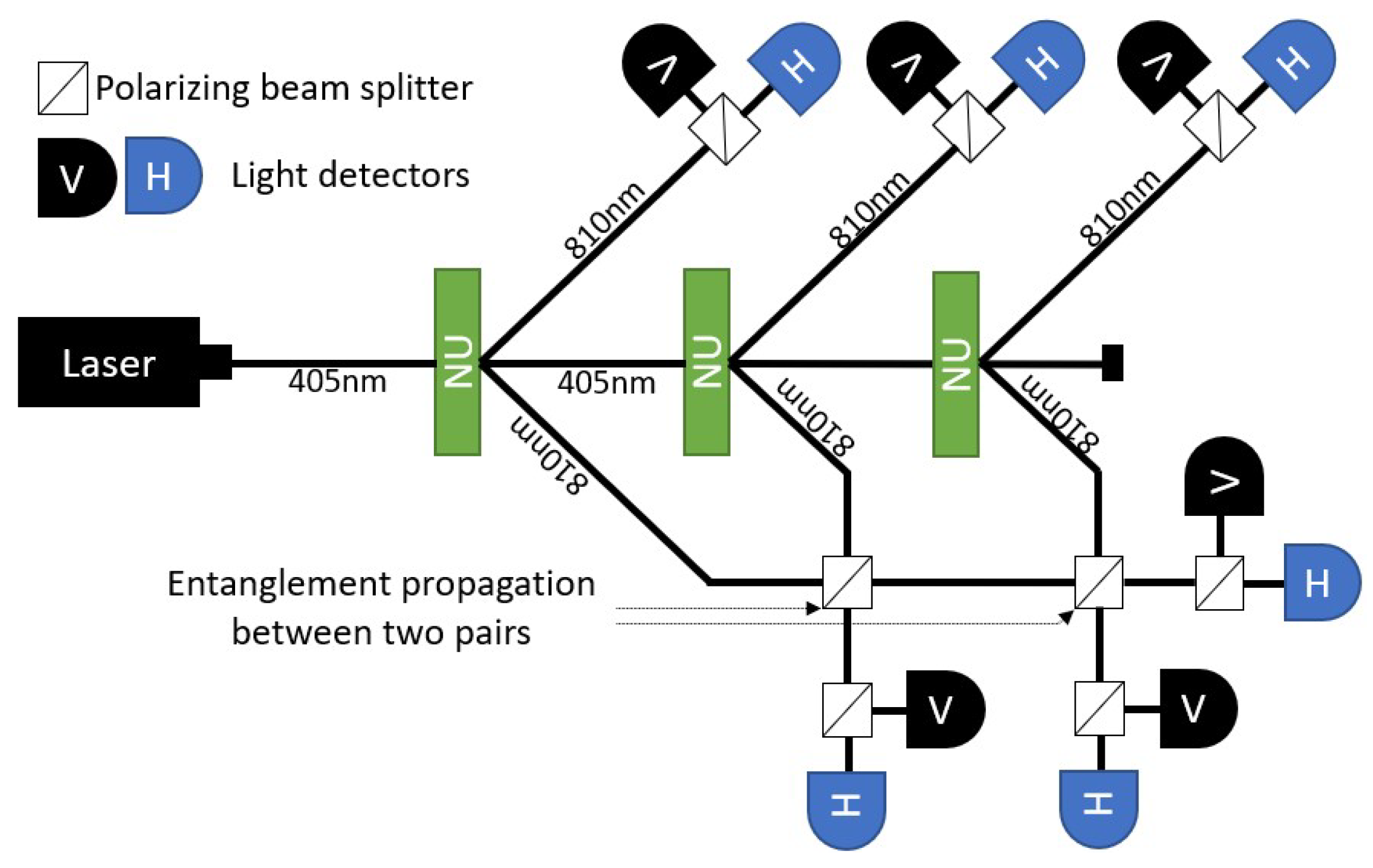
This technique, depicted in Figure 1, creates $\frac{n}{2}$ pairs of photons using nonlinear units such as BBO or ultra-thin films, in series. Following the creation of the pairs, entanglement is propagated by $\frac{n}{2}$ polarizing beam splitters. Each splitter connects the corresponding entanglement with the next pair generated. We used a similar setup, but required more states than provided by GHZ for computation. Hence, we connected both sides of the output from each nonlinear unit using non-polarizing beam splitters. The states created by this setup were highly interesting from a quantum computation perspective.

3.1. Experimental Setup for QCoSamp

Consider applying a 50:50 beam splitter to the state described in Equation (8). The corresponding setup is shown in Figure 2. Given the input state is ${|1,1\rangle }_F$, we can apply Equation (4). The parameter $\theta$ takes the value $\pi /4$, giving $cos\left(2\theta \right)=0$ and $sin\left(2\theta \right)=1$. For simplicity, we assume that the phase $\delta$ is equal to zero. Note that this will not be the case for the real system without specific intervention. This will be described in the calibration section. In rail-polarization (RP) notation, defined in Figure 2 (right), the Magnitskiy equation (Equation (8)) becomes (For one NU, we have two rails, and hence, the RP state has four slots. For simplicity, we omit the vacuum state of the remaining rail, since it is not involved in the process):

$$\frac{1}{\sqrt{2}}\left(|10,01\rangle +|01,10\rangle \right).$$

(10)

As shown in Figure 3, we denote the creation operators for the first input of the beam splitter as ${\widehat{a}}_h^{†}$ and ${\widehat{a}}_v^{†}$, for horizontally and vertically polarized photons, respectively. For the second input, we use ${\widehat{b}}_h^{†}$ and ${\widehat{b}}_v^{†}$; for the first output, we use ${\widehat{c}}_h^{†}$ and ${\widehat{c}}_v^{†}$; for the second output, we use ${\widehat{d}}_h^{†}$ and ${\widehat{d}}_v^{†}$.

We now provide a list of all two and four creation operators for reference during the remainder of this work. For convenience, we omit the proofs; each operator can be derived straightforwardly by expanding Equation (5), as they commute with one another. We assume that a 50:50 beam splitter is used, with a phase shifter on one output with relative phase $\phi$. The operators are as follows:

$$\begin{array}{cc}\hfill {\widehat{a}}_h^{†}{\widehat{b}}_v^{†}& =-\frac{1}{2}i\left(e^{i\phi }{\widehat{c}}_h^{†}{\widehat{c}}_v^{†}+e^{-i\phi }{\widehat{d}}_h^{†}{\widehat{d}}_v^{†}\right),\hfill \\ \hfill {\widehat{a}}_v^{†}{\widehat{b}}_h^{†}& =-\frac{1}{2}i\left(e^{i\phi }{\widehat{c}}_h^{†}{\widehat{c}}_v^{†}+e^{-i\phi }{\widehat{d}}_h^{†}{\widehat{d}}_v^{†}\right),\hfill \\ \hfill {\widehat{a}}_h^{†}{\widehat{b}}_h^{†}& =-\frac{1}{2}i\left(e^{i\phi }{\left[{\widehat{c}}_h^{†}\right]}^2+e^{-i\phi }{\left[{\widehat{d}}_h^{†}\right]}^2\right),\hfill \\ \hfill {\widehat{a}}_v^{†}{\widehat{b}}_v^{†}& =-\frac{1}{2}i\left(e^{i\phi }{\left[{\widehat{c}}_v^{†}\right]}^2+e^{-i\phi }{\left[{\widehat{d}}_v^{†}\right]}^2\right),\hfill \\ \hfill {\widehat{a}}_h^{†}{\widehat{a}}_v^{†}& =\frac{1}{2}\left({\widehat{c}}_h^{†}{\widehat{c}}_v^{†}-i{e}^{-i\phi }{\widehat{c}}_h^{†}{\widehat{d}}_v^{†}-i{e}^{-i\phi }{\widehat{c}}_v^{†}{\widehat{d}}_h^{†}-e^{-i2\phi }{\widehat{d}}_h^{†}{\widehat{d}}_v^{†}\right),\hfill \\ \hfill {\widehat{b}}_h^{†}{\widehat{b}}_v^{†}& =\frac{1}{2}\left({\widehat{d}}_h^{†}{\widehat{d}}_v^{†}-i{e}^{-i\phi }{\widehat{c}}_h^{†}{\widehat{d}}_v^{†}-i{e}^{-i\phi }{\widehat{c}}_v^{†}{\widehat{d}}_h^{†}-e^{-i2\phi }{\widehat{c}}_h^{†}{\widehat{c}}_v^{†}\right),\hfill \\ \hfill {\widehat{a}}_h^{†}{\widehat{a}}_v^{†}{\widehat{b}}_h^{†}{\widehat{b}}_v^{†}& =-\frac{1}{4}\left(e^{i2\phi }{\left[{\widehat{c}}_h^{†}\right]}^2{\left[{\widehat{c}}_v^{†}\right]}^2+{\left[{\widehat{c}}_h^{†}\right]}^2{\left[{\widehat{d}}_v^{†}\right]}^2+{\left[{\widehat{c}}_v^{†}\right]}^2{\left[{\widehat{d}}_h^{†}\right]}^2+e^{-i2\phi }{\left[{\widehat{d}}_h^{†}\right]}^2{\left[{\widehat{d}}_v^{†}\right]}^2\right).\hfill \end{array}$$

(11)

To complement the operators, we also provide a list of state transformations required by our model:

$$\begin{array}{cc}\hfill |10,01\rangle \stackrel{\mathrm{BS}}{\to }& -\frac{1}{2}i\left(e^{i\phi }|11,00\rangle +e^{-i\phi }|00,11\rangle \right),\hfill \\ \hfill |01,10\rangle \stackrel{\mathrm{BS}}{\to }& -\frac{1}{2}i\left(e^{i\phi }|11,00\rangle +e^{-i\phi }|00,11\rangle \right),\hfill \\ \hfill |10,10\rangle \stackrel{\mathrm{BS}}{\to }& -\frac{1}{2}i\left(e^{i\phi }|20,00\rangle +e^{-i\phi }|00,20\rangle \right),\hfill \\ \hfill |01,01\rangle \stackrel{\mathrm{BS}}{\to }& -\frac{1}{2}i\left(e^{i\phi }|02,00\rangle +e^{-i\phi }|00,02\rangle \right),\hfill \\ \hfill |11,00\rangle \stackrel{\mathrm{BS}}{\to }& \frac{1}{2}\left(|11,00\rangle -i{e}^{-i\phi }|01,10\rangle -i{e}^{-i\phi }|10,01\rangle -e^{-i2\phi }|00,11\rangle \right),\hfill \\ \hfill |00,11\rangle \stackrel{\mathrm{BS}}{\to }& \frac{1}{2}\left(|00,11\rangle -i{e}^{-i\phi }|01,10\rangle -i{e}^{-i\phi }|10,01\rangle -e^{-i2\phi }|11,00\rangle \right),\hfill \\ \hfill |11,11\rangle \stackrel{\mathrm{BS}}{\to }& -\frac{1}{4}\left(|20,02\rangle +|02,20\rangle +e^{i2\phi }|22,00\rangle +e^{i2\phi }|00,22\rangle \right).\hfill \end{array}$$

(12)

Using the above states and transformations, the action of a 50:50 beam splitter with $\phi =0$ on the output of a nonlinear unit is given by

$$\frac{1}{\sqrt{2}}\left(|10,01\rangle +|01,10\rangle \right)\stackrel{\mathrm{BS}}{\to }\left[\frac{1}{\sqrt{2}}({\widehat{a}}_h^{†}{\widehat{b}}_v^{†}+{\widehat{a}}_v^{†}{\widehat{b}}_h^{†})\right]|0\rangle =-\frac{1}{\sqrt{2}}i\left(|11,00\rangle +|00,11\rangle \right)=|\Psi \rangle .$$

(13)

This equation shows that the two entangled photons that leave the nonlinear unit on different rails will both be on either the “left” or “right” rail after they pass through the beam splitter. However, the original state, given by Equation (8), does not change.

The MSO (Figure 2) consists of two such operations. Hence, at the output, there are four rails and four photons, entangled in pairs. As such, the final output state $|MSO\rangle$ is a tensor product of the states $|{\Psi }_1\rangle$ and $|{\Psi }_2\rangle$, corresponding to the first and second nonlinear unit, respectively. Therefore, we can write the final state of the MSO as follows:

$$\begin{array}{cc}\hfill |MSO\rangle =& |{\Psi }_1\rangle \otimes |{\Psi }_2\rangle =\hfill \\ \hfill =& -\frac{1}{2}\left(|11,00;11,00\rangle +|11,00;0011\rangle +|00,11;11,00\rangle +|00,11;00,11\rangle \right).\hfill \end{array}$$

(14)

We have so far assumed that no differences in the light phase arise between the nonlinear units and the beam splitters. However, this is infeasible in practical applications. To compensate for the phase differences that do arise, we apply adjustable phase shifters at the outputs of both beam splitters, as shown in Figure 2. Each adjustable phase shifter is implemented using an electro-optic phase modulator, which shifts the phase of light in the range $[-\pi ,\pi ]$. The shift is a linear function of the applied voltage. We refer to this compensation process as the setup calibration. Given that the optical paths are separate at this stage, calibration can be performed for each of them independently. However, the relative phase is not measurable directly, as both states in Equation (13) can be obtained with equal probability. Therefore, we must use the Mach–Zehnder interferometer [25,26,27] to extract the phase. The calibration procedure then takes place over two steps:

• The optical path for a given nonlinear unit is extended by the Mach–Zehnder interferometer;
• The light phase is calibrated using the adjustable phase shifter until both outputs from the interferometer have the same intensity.

This calibration process must be performed whenever the setup is modified or if a long period of time has passed since the previous calibration.

3.2. Implementation of the QCoSamp Component Using the MSO

In this section, we present the implementation and combination of the QCoSamp components. Figure 4 shows an optical path consisting of two QCoSamp components. The path begins with a pre-prepared and calibrated MOS, which has four output rails. The state of the MSO is given by Equation (14). Output rails 1 and 2 contain one entangled photon pair; output rails 3 and 4 contain the other. Hence, we have two independent entangled systems. Using the method of Wang et al. [23] and Zhong et al. [24], the entanglement is propagated throughout the entire system using two beam splitters (indicated in yellow and green). On one output rail of each beam splitter is a phase shifter that introduces the parameters $\phi$ and $\gamma$. Next, the rails that contain the horizontally and vertically polarized photons are divided with polarizing beam splitters. This ensures that each separate rail contains photons of the same polarization. The rails are then measured with photo detectors to obtain the state, in the manner indicated at the bottom of the figure. As considered in state notation in the Fock space, this leads to the connection of the inner two pairs (indicated in green) and the connection of the outer two pairs (indicated in yellow).

The action of the beam splitters on two of the four pairs leaves the remainder of the state unaltered. Consider the beam splitter acting on the inner two pairs of the state $|11,00;11,00\rangle$, that is the state $|·,00;11,·\rangle$. By applying the corresponding transformation for the state $|00,11\rangle$, given by Equation (12), we obtain

$$|·,00;11,·\rangle \stackrel{\mathrm{BS}}{\to }\frac{1}{2}\left(|·,00;11,·\rangle -i{e}^{-i\phi }|·,01;10,·\rangle -i{e}^{-i\phi }|·,10;01,·\rangle -e^{-i2\phi }|·,11;00,·\rangle \right).$$

(15)

Now, consider the beam splitter acting on the outer two pairs, that is $|11,·;·,00\rangle$. This gives the output

$$|11,·;·,00\rangle \stackrel{\mathrm{BS}}{\to }\frac{1}{2}\left(|11,·;·,00\rangle -i{e}^{-i\phi }|01,·;·,10\rangle -i{e}^{-i\phi }|10,·;·,01\rangle -e^{-i2\phi }|00,·;·,11\rangle \right).$$

(16)

Connecting these two states together forms an all-to-all connection of both output states for which the coefficients are multiplied, as shown in the first table in Figure 4 (right). The second table shows the same operation for the state $|00,11;00,11\rangle$. Both input states $|11,00;11,00\rangle$ and $|00,11;00,11\rangle$ produce the same output state list with different coefficients. The coefficients are functions of the relative phases, $\phi$ and $\gamma$. This is a key observation: the coefficients of the same output state will sum, and hence, measuring the state will extract the difference in phase, in the same manner as the final Hadamard operation in QCoSamp. Consider the state $|00,01;10,11\rangle$, shown in cell $(1,2)$ of the tables in Figure 4 (right), highlighted in yellow. This state has the coefficient $i{e}^{i(-2\gamma +\phi )}-i{e}^{-i\phi }=i{e}^{-i\phi }(e^{-i2\phi }-1)$. The probability (Normalization is omitted for simplicity. To obtain the correct probability, the normalization coefficients must be included: $\frac{1}{2}$ from the last two equations and $-\frac{1}{2}$ from the output state of the MOS, giving a normalization factor of $\frac{1}{16}$.) of obtaining this state is hence given by $i{e}^{-i\phi }(e^{-i2\phi }-1)·-i{e}^{i\phi }(e^{i2\phi }-1)=2-2cos\left(2\phi \right)$. If we assume that $x=2\phi$, we obtain the value of the QCoSamp component.

The third table in Figure 4 (right) lists the probabilities (again, normalization omitted for simplicity) obtained for each corresponding state. Our setup encodes five functions, as indicated by the repeating values. Although any functions and the sums thereof can be extracted, the important cells are highlighted in yellow and green.

The remaining two states, $|11,00;00,11\rangle$ and $|00,11;11,00\rangle$, transform as follows:

$$|11,11\rangle \stackrel{\mathrm{BS}}{\to }-\frac{1}{4}\left(|20,02\rangle +|02,20\rangle +e^{i2\phi }|22,00\rangle +e^{i2\phi }|00,22\rangle \right).$$

(17)

These states will not sum correctly because of the obtained factor of 2 in the crossed sections. Hence, the phases cannot be obtained. The probability of obtaining each state will be equal to $\frac{1}{16}$. Given that there are eight such states, one of them will be obtained with $\frac{1}{2}$ probability. We omit these states from our calculations and treat them as noise.

We can observe the first and second ququartit in the above representation. The probability distribution obtained for these ququartits can be summed for the basis states |01〉 and |02〉, for the parameter $\phi$, and |31〉 and |32〉, for the parameter $\gamma$.

Now, we apply the values of x, $2x$, r, and s to the top-left, top-right, bottom-left, and bottom-right phase shifters, respectively (as shown in Figure 4). By multiplying the resulting probability distributions by 4, we obtain the final function:

$$\mu \left(x\right)=\frac{1+cos(x+r)}{2}+\frac{1+cos(2x+s)}{2}.$$

(18)

This function embodies two-component QCoSamp.

Further development of the system is possible by adding more nonlinear units to the MOS. Each additional nonlinear unit provides a further two rails, along which the entanglement should propagate. This can be achieved by using two additional beam splitters following the original two. The two rails from the third nonlinear unit should merge with rail 4 and rail 1, as shown in Figure 4. By adding nonlinear units in this manner, the number of QCoSamp components can be increased. The addition of two nonlinear units generates one new component.

4. Discussion and Conclusions

In this paper, we demonstrated the construction of an optical setup that creates a single component for the QCoSamp operator. We further demonstrated how the inclusion of additional components can create a series, as described in a previous work [4]. To conclude the demonstration, we must indicate the section of the optical path that forms a single QCoSamp component and the method by which additional components can be added. However, due to the nature of our system, the components are not clearly delineated. The beam splitters applied to the output of the MOS and the attached phase shifters approximately designate a single component; by changing the phase of the phase shifters, the argument of the component can be modified. Additional components can be incorporated via the inclusion of more nonlinear units, as described in the previous section. This addition results in further propagation of the entanglement.

The limitations of optoelectronic devices will soon be met, due to the high complexity and relatively long distances between consecutive devices, among other factors. These problems can be overcome with the use of photonic chips. The introduction of such chips will be analogous to the introduction of the first silicon chips. Such photonic technology is still in the early stages of development, and further miniaturization of photonic devices is expected. Using photonic chips in place of trapped ion devices, or similar, provides a substantial advantage due to the ability of the technology to operate at room temperature. Moreover, algorithms such as amplitude amplification must iterate many times using the same gates. This can be implemented by generating a loop in the light trajectory, rapidly increasing the quantum volume of such devices without the need to implement many additional gates.

Our proposed implementation using optical quantum phenomena does not share the same problems as implementations such as KML, as we utilized entanglement as a resource for quantum computation, in addition to a tool for constructing control gates via entanglement between qubits. The QCoSamp parameters are controlled using entanglement: a change in the phase of one rail via the phase shifter of another rail is possible because of entanglement. Hence, the use of nonlinear units is wider than in other solutions—such units both create entanglement between qubits and control the system.

To avoid problems with accurate result detection, we rejected the use of the heralding technique. Instead, we considered only temporally correlated photons; one on each rail. Although this approach decreases the efficiency of the system, it increases the fidelity. The decrease in efficiency can be remedied by the application of a high-efficiency entangled photon source, such as ultra-thin films or quantum dots.

It is important to note that the theoretical results presented in this paper pave the way for the implementation of advanced methods within photonic chips. Using this framework, the algorithms from the areas of signal processing, image processing, feature extraction, and image classification can be implemented on photonic circuits.

Moreover, the described setup offers additional possible outputs. The table of probability shown in Figure 4 presents alternative functions of x, r, and s, such as $4co{s}^2(x-y)$. By measuring the first and third ququartits, we generate the probability for basis state |11〉. This creates the opportunity to generate additional series that can be used for optimization algorithms.

This work engenders further research in several areas.

• The detection of the temporal correlation of four or more photons in two polarization states. Our setup requires a specific detector for the ququartits’ states. For example, the state |00〉 must be detected by observing the remainder of the system. However, states with two photons on the same rail with the same polarization, such as |20〉, were rejected, as they are not required for computations.
• The implementation of distributed phase encoding [4,15], which is required for the implementation of quantum algorithms such as quantum summation [28] or optimization [29].
• The implementation of the amplitude amplification algorithm [16,17], which forms the core of the optimization methods that can be applied in QCoSamp.