Numerical Simulation and Evaluation on Continuum Damage Models of Rocks

Abstract

Damage mechanics play an important role in the analysis of rock deformation and failure. Numerous damage variables have been proposed and the corresponding continuum damage models were suggested. Knowing how to apply these theoretical models appropriately in numerical simulations is the key to whether they can be adopted to solve practical problems. The continuum damage models were grouped into empirical damage models, statistical damage models, and elastoplastic damage models in this article. Their applicability and limitations were studied according to some numerical simulations of the most basic uniaxial compression test of a cylinder rock sample. Three representative damage models were chosen from the literature and applied to FEM numerical simulations by introducing a self-developed program. The stress-strain curves due to damage were obtained from the numerical simulation results and compared to those from the experimental results. The damage distribution and evolution of different damage models were investigated to evaluate their influences on rock deformation. It can be concluded that strain-softening stages presented by both the empirical damage models and the statistical damage models are caused by subtracting the elastic modulus gradually while those presented by the elastoplastic damage models are caused by reducing plastic yield stress gradually. Damage-elastic coupling cannot well reflect the irreversibility of damage. The elastoplastic damage models combine damage with plastic history, and thus the irreversibility of damage can be represented. Furthermore, the compulsory reduction of the elastic modulus can probably lead to extreme element distortion and even an unreasonable negative modulus when damage is very serious, which inevitably causes the numerical simulation to fail prematurely under complex stress states. Although the elastoplastic damage models are recommended at present rather than the other models, a more appropriate definition of the damage variable can be expected that should track the whole deformation and failure process. Knowing how to treat the adverse effect of local deterioration due to damage is the challenge numerical simulations have to face when they are applied in the actual project with complex stress states.

1. Introduction

All kinds of engineering construction and evaluation activities are closely related to the rock destruction process. However, rock is a kind of natural geological material with a very complex interior structure. There are a large number of cracks, pores, joints, inclusions, and other natural defects in rock, and thus rock is a discontinuous, heterogeneous, and anisotropic medium [1]. In addition, lots of external factors, such as geological location, hydrological characteristics, geo-stress distribution, temperature conditions, and mining sequences, also affect the damage and deformation characteristics of rock. Essentially, the rock failure process often has significant localized characteristics owing to the initiation and expansion evolution of inner micro-defects [2,3]. The study of rock deformation and failure is extremely complicated and has become one of the key problems studied by scientists and technicians [4]. More and more mechanical models revising constitutive relations and failure criteria have been proposed [5]. Among them, the models based on damage mechanics which can better explain rock failure processes have drawn more attention.

Damage mechanics is an important subject and a powerful tool for rock research. It mainly studies macroscopic mechanical effects caused by the generation and development of internal defects of solid materials under certain load and environmental conditions [6]. As early as 1958, Kachanov [7] proposed the concepts of a continuity factor and effective stress in his study on metal creep. In 1963, Rabotnov [8] defined the concept of a damage factor and established the constitutive equation and evolution equation of damage. In 1976, the topic of damage mechanics was first introduced into the study of rock mechanics. Up to now, researchers have proposeddifferent definitions of damage variables including scalar, vector, or tensor forms [9,10,11,12,13,14,15]. Damage mechanics theory can be grouped into macro-damage theory, meso-damage theory, and micro-damage theory according to its characteristic scale. The macro-damage theory is also called continuum damage. It studies the effect of damage from the viewpoint of phenomenological investigation. The physical mechanism of damage and the specific change of the mesostructure are neglected. It is widely adopted because of the mature theoretical system and good macroscopic response.

Many damage models have been suggested. Loland [16] proposed a segmental damage model and regarded that microcracks emerged in the pre-peak stage and the damage mainly occurred in the post-peak stage. Mazars [17] established a continuous damage model by fitting stress-strain curves under the background of concrete. Xie and Ju [18] defined a damage variable by considering the fractal dimension effect and raised a damage model in the framework of nonequilibrium thermodynamics. Shen and Tang [19] derived a statistical damage model for brittle rocks based on the Weibull distribution and uniform strength criteria. Bruning and Karakus [20] believed that damage and plasticity were closely coupled and proposed an elastoplastic damage model in a double exponential form. A plastic-damage model driven by the physical mechanisms of microcracks growth and pore collapse was proposed to describe the mechanical behavior under high pressure [21]. Generally, the purpose of these models is to reproduce the mechanical response and describe the rock failure process exactly. The validation of them usually focused on whether they can agree with experimental stress-strain curves well. However, the question of how to use these models was less discussed.

The processes of rock deformation and failure are complicated. Numerical simulation is the major method for an actual project with complex stress states. Knowing how to apply damage models in numerical simulations is crucial in order to realize the effect of damage on rock deformation calculations and failure judgement. The mechanical properties of rock involve not only stress-strain behavior, but also the distribution and evolution of damage and deformation inside. The limitations and applicability of different rock damage models were less discussed previously. Therefore, some representative damage models will be introduced into FEM numerical simulations and compared carefully in order to better evaluate them.

The remainder of this paper is organized as follows. The theoretical foundations of three representative rock damage models are presented in Section 2. The numerical simulation schemes, including numerical parameters, boundary conditions, and calculated programs, are stated in Section 3. The results and discussion are studied in Section 4. The conclusions are finally drawn in Section 5.

2. Theory Foundations of Damage Models

Most rock damage models were established based on elastic-damage coupled or elastic-plastic-damage coupled mechanisms. In these models, some were presented by fitting experimental results [22], some were put forward via statistical theory [23,24], and some were deduced using nonequilibrium thermodynamics or traditional elastic-plastic theory [25,26,27]. These models can be grouped into empirical damage models, statistical damage models, and elastoplastic damage models.

2.1. The Empirical Damage Models

The empirical damage models were established by experimental fitting in which only the elastic-damage coupling mechanism was considered. After a damage variable was proposed, it was used to degrade the elastic modulus of the damaged rocks according to

$$E=E_0\left(1-D\right)$$

(1)

and then the degraded elasticity modulus was substituted into generalized Hooke’s law to match the stress-strain curve of a specific sample; the constitutive equation was

$${\sigma }_1=E_0{\epsilon }_1\left(1-D\right)+2\upsilon {\sigma }_3$$

(2)

where E₀ is the initial elastic modulus; E is the damaged elastic modulus; υ is the Poisson’s ratio; D is the damage variable; σ₁ is the first principal stress; ε₁ is the first principal strain; and σ₃ is the third principal stress.

In this kind of model, the damage variable was always written as an expression of stress or strain. Here, the expression of strain in reference [28] was adopted as

$$D={\left(\epsilon /{\epsilon }_s\right)}^n$$

(3)

where ε is the axial strain value; ε_s, and n are material constants.

Thus, the constitutive equation could be obtained by substituting Equation (3) into Equation (4) as

$${\sigma }_1=E_0{\epsilon }_1\left[1-{\left(\epsilon /{\epsilon }_s\right)}^n\right]+2\upsilon {\sigma }_3$$

(4)

It should be figured out that the confining pressure σ₃ = 0 under uniaxial conditions. It also can be applied to uniaxial conditions. Generally, no failure criterion was introduced in the empirical damage model. It only adopted a damage variable to reduce the elastic modulus and was calculated by generalized Hooke’s law, and the strain-softening stage emerged because of the gradually decreasing elastic modulus.

In addition, the damage variable could also be defined as the energy ratio [29] or the introduced coefficient [30], or in piecewise forms [16] to simulate the stress-strain curves.

2.2. The Statistical Damage Models

The statistical damage models were deduced according to statistical theory. In these models, the mechanical parameters of micro-elements were assumed to obey a certain probability distribution function, such as the Weibull distribution, normal distribution, and uniform distribution. The damage value was defined as the quantity ratio of failure microelements to total microelements and then substituted into generalized Hooke’s law to form a constitutive equation. The mechanical parameters that obey statistical distribution can be chosen as strength [31,32,33], cohesion [34], energy [35], etc. The failure criteria to judge whether microelements need to be damaged can be designated as the M-C criterion, D-P criterion, Hooke–Brown criterion, energy criterion, and so on.

Taking the model in the reference [36] as an example, the strength parameter of the micro-elements was assumed to obey the Weibull distribution, and the micro-elements’ strength satisfied the M-C criterion. The probability density function is

$$P\left(F\right)=\{\begin{array}{ll}\frac{m}{F_0}{\left(\frac{F}{F_0}\right)}^{m-1}\exp \left[-{\left(\frac{F}{F_0}\right)}^m\right]\hfill & F>0\hfill \\ 0\hfill & F⩽0\hfill \end{array}$$

(5)

where F is the strength of the micro-elements, and F₀ and m are the Weibull distribution parameters.

Therefore, the damage variable is represented as

$$D=\frac{N_f}{N}=\frac{{\int }_0^{F}NP\left(x\right)dx}{N}=\frac{N\left\{1-\exp \left[-{\left(\frac{F}{F_0}\right)}^m\right]\right\}}{N}=1-\exp \left[-{\left(\frac{F}{F_0}\right)}^m\right]$$

(6)

where N is the total microelements number and N_f is the number of failure microelements.

The effective stress sustained by the undamaged area was equal to the apparent stress calculated by the whole area.

$${\sigma }_i^{*}=\frac{{\sigma }_i}{\left(1-D\right)} \left(i=1,2,3\right)$$

(7)

where ${\sigma }_i^{*}$ is the effective stress, and I = 1, 2, 3.

As for the triaxial compressive tests, the relationship between axial stress and strain based on Hooke’s law is:

$${\sigma }_1^{*}=E_0{\epsilon }_1+\upsilon \left({\sigma }_2^{*}+{\sigma }_3^{*}\right)$$

(8)

Substituting Equation (7) into Equation (8) produces:

$$\left(1-D\right)=\frac{{\sigma }_1-\upsilon \left({\sigma }_2+{\sigma }_3\right)}{E_0{\epsilon }_1}$$

(9)

In Equation (6), $F$ is the strength of the micro-elements, and the values are different in various micro-elements because of the heterogeneity of rock materials. The micro-element will be destroyed when the strength criterion can be satisfied, so the $F$ can be shown in Equation (10) if the M-C criterion was used.

$$F=f\left(\sigma \right)=\left({\sigma }_1^{*}-{\sigma }_3^{*}\right)-\left({\sigma }_1^{*}+{\sigma }_3^{*}\right)\sin \phi =\frac{E_0{\epsilon }_1\left[\left({\sigma }_1-{\sigma }_3\right)-\left({\sigma }_1+{\sigma }_3\right)\sin \phi \right]}{{\sigma }_1-\upsilon \left({\sigma }_2+{\sigma }_3\right)}$$

(10)

where φ is the internal friction angle.

Combined with the generalized Hooke’s law and Equations (6)–(10), the constitutive equation is established as

$${\sigma }_1=E_0{\epsilon }_1\left\{\exp \left[-{\left(\frac{F}{F_0}\right)}^m\right]\right\}+2\upsilon {\sigma }_3$$

(11)

To consider the residual stress effect, residual coefficient c_n [36] could be introduced into Equation (11), and the damage variable could be expressed as

$${\sigma }_1=E_0\left(1-c_{n}D\right)+2\upsilon {\sigma }_3=E_0{\epsilon }_1\left\{\left(1-c_n\right)+c_n\exp \left[-{\left(\frac{F}{F_0}\right)}^m\right]\right\}+2\upsilon {\sigma }_3$$

(12)

where c_n is the residual coefficient.

It should be figured out that the confining pressure σ³ = 0 under uniaxial conditions. It also can be applied to uniaxial conditions. In the statistical damage model, it also introduced the damage variable to reduce the elastic modulus and was calculated by generalized Hooke’s law. However, the strength of micro-elements was assumed to obey the Mohr–Coulomb criterion. Therefore, the Mohr–Coulomb criterion was considered in the statistical damage model, but it still was an elastic-damage model.

In recent years, the statistical damage model has been widely used by combining hydraulic damage [37,38,39], the fracture mechanics model [40], the temperature damage [23,41], the dynamic damage [42,43], etc.

2.3. The Elastoplastic Damage Models

Unlike the empirical and statistical damage models, the elastoplastic damage models were deduced by considering the elastic-plastic-damage coupling effect. Many elastoplastic damage models were deduced using traditional plastic mechanics theory or nonequilibrium thermodynamics [25,26]. Under the traditional plastic mechanics theory, a softening model was introduced into the plastic internal variable to describe the softening behaviors of materials [44]. However, the degradation mechanism due to microcrack initiation was ignored. Therefore, the damage variable was substituted to reduce the elasticity modulus and hardening function [20,25,45].

When coupling damage with elasticity and plasticity, the stress-strain relationship can be expressed as

$$\Delta \sigma =\left(1-D\right)E_0\left(\Delta \epsilon -\Delta {\epsilon }^p\right)$$

(13)

where Δσ is the stress increment, Δε is the total strain increment, and Δε^p is the plastic strain increment.

In the reference [25,45], the plastic yield function took D-P criterion, and the damage-plasticity yield function and potential function are

$$f\left(\sigma ,k,D\right)=\alpha I_1+\sqrt{J_2}-\left(1-D\right)k$$

(14)

$$g\left(\sigma ,k,D\right)=\beta I_1+\sqrt{J_2}-\left(1-D\right)k$$

(15)

where I₁ is the first invariant of the nominal stress; $J_2=\frac{1}{2}s:s, s=\left(\sigma -\frac{I_1}{3}I\right)$ is the second invariant of the nominal deviatoric stress, and $k$ is the hardening function; α is friction parameter, and β is dilatation parameter.

After introducing a plastic multiplier Δλ, the plastic strain increment was determined by

$$\Delta {\epsilon }^p=\Delta \lambda \frac{\partial g\left(\sigma ,k,D\right)}{\partial \sigma }=\Delta \lambda \left[\alpha I_1+\frac{s}{2\sqrt{J_2}}-\left(1-D\right)\frac{\partial k}{\partial \sigma }\right]$$

(16)

The loading and unloading criterion are

$$f\left(\sigma ,k,D\right)\le 0,\Delta \lambda \ge 0,f\left(\sigma ,k,D\right)\Delta \lambda =0$$

(17)

The hardening function is

$$k={\sigma }_0+k_c,{\sigma }_0=6c\cos \phi /\left[\sqrt{3}\left(3-\sin \phi \right)\right]$$

(18)

where k_c is the plastic internal variable; it was shown in the reference [46] as

$$k_c=a_1\lambda \exp \left(a_2{I}_1-a_3\lambda \right)$$

(19)

where a₁, a₂, and a₃ are constants.

To consider the effect of microcrack propagation, the damage variable [45] was expressed as

$$D=1-\exp \left(-a{\epsilon }_v\right)$$

(20)

where ε_v is the volumetric strain and a is the model parameter. It should be noted that ε_v has a positive value to represent volume expansion.

Apparently, the strain softening in the post-peak stage can be obtained using the above damage models, respectively. However, such a descent of a stress-strain curve needs to be evaluated prudently. According to Equations (1)–(20), the theoretical stress-strain curves can be plotted and the calculating principles of the damage effect are illustrated in Figure 1.

There is only a damage-elastic coupling mechanism in the empirical damage model and statistical damage model. From Figure 1a,b, it is indicated that the stress descent is caused by reducing the elastic modulus. The elastic modulus at each point is calculated according to the secant modulus in these damage-elastic coupling models. Therefore, the stress descent is obtained with the increase in damage and might recover once the stress, strain, or other parameters defining damage decrease. It cannot reflect the irreversibility of damage well. The calculating principle in the elastoplastic damage model is illustrated in Figure 1c. The incremental method is adopted when introducing the plastic calculation. In the pre-peak stage before the plastic yield, the stress increment Δσ depends on the degraded elastic modulus due to damage. It decreases with the increase in damage, and thus causes the stress-strain curve to bend downward. Once a plastic yield function has been satisfied, the stress increment Δσ depends on the plastic hardening function and a certain plastic deformation happens. The yield stress decreases with the increase in damage, and thus a negative stress increment is obtained which causes the stress-strain curve to descend. In the classical plastic stage without damage, the total strain increment is the sum of elastic strain and plastic strain. However, in the post-peak stage after the plastic yield coupling with damage, the total strain increment is derived by subtracting elastic strain from plastic strain, i.e., Δε = Δε^p − Δε^e. Although the elastic modulus is also degraded, the descent of the stress-strain curve is supposed to be caused by the reduction of yield stress. The elastic damage can only affect the steepness of such a descent slightly. Because damage is coupled with plastic that tracked with irreversible plastic deformation, the irreversibility of damage can also be represented.

3. Numerical Simulation Scheme

3.1. Representative Models

As mentioned above, rock damage models can be grouped into the empirical damage models, the statistical damage models, and the elastoplastic damage models. Three representative models were chosen for numerical simulation and discussion. The damage variable and coupling mechanism of different models are listed in

Table 1. The summary of calculated models.

Type	Damage Variable	Coupling Mechanism	Applicable
Empirical damage model	$\mathrm{Some} \mathrm{empirical} \mathrm{definitions} \mathrm{based} \mathrm{on} \mathrm{experimental} \mathrm{results}, \mathrm{e}.\mathrm{g}., D={\left(\frac{\epsilon }{{\epsilon }_s}\right)}^n$ [28]	$E=\left(1-D\right)E_0$	Proposed according to total amount of stress and strain. Not applicable to local elastic unloading.
Statistical damage model	$\mathrm{Effects} \mathrm{of} \mathrm{probability} \mathrm{distribution} \mathrm{of} \mathrm{micro} \mathrm{elements}, \mathrm{e}.\mathrm{g}., D=1-\exp \left[-{\left(\frac{F}{F_0}\right)}^m\right]$ [36]	$E=\left(1-D\right)E_0$	Proposed according to total amount of stress and strain. Not applicable to local elastic unloading.
Elastoplastic damage model	$\mathrm{Mechanisms} \mathrm{of} \mathrm{elastic} \mathrm{and} \mathrm{plastic} \mathrm{deformation}, \mathrm{e}.\mathrm{g}., D=1-\exp \left(-a{\epsilon }_V\right)$ [45]	$E=\left(1-D\right)E_0$$f\left(\sigma ,k,D\right)=\alpha I_1+\sqrt{J_2}-\left(1-D\right)k$	Proposed according to stress and strain increment. Reflect whole deformation histories by plastic strains. Can be calculated in unloading process.

.

In the empirical damage model, the parameter εs should be larger than the ultimate value of axial strain. Otherwise, the elastic modulus will become negative. In the statistical damage model, model parameters m and F₀ are the Weibull distribution parameters that can be obtained by the fitting or extremum method [41]. The parameter F₀ is considered as the average value of strength. The shape parameter m is regarded as the uniformity factor of rocks that reflect the concentration degree of strength around a certain value. The residual stress level was controlled by the model parameter c_n. In the elastoplastic damage model, damage occurs when the volume begins to inflate, and thus the negative volume strain indicating compression needs to be truncated as zero. The damage variable affects both the elastic modulus and hardening function. The model parameter a can be obtained by fitting and the regression of some experimental data [45].

3.2. Numerical Model and Parameters

In this paper, the FEM software COMSOL Multiphysics was used for numerical calculations. The procedures in COMSOL Multiphysics mainly include the definition of strong form governing equations of each involved physical field and the setup of the solver. It has various extension interfaces for users to modify the computational item conveniently. Here, the solid mechanics module was used and calculated by introducing different definitions of damage variables. A three-dimensional cylinder model with a diameter of 50 mm and a height of 100 mm was constructed and simulated under uniaxial compression. The numerical model has 1900 elements, and the type of element is a hexahedron element in FEM.

Two kinds of boundary conditions were considered. One is an ideal case in which the horizontal direction of end restrain was set to be free and the model was uniformly compressed, which is also the situation that was expected in experimental studies. In this case, the stress and strain in the whole sample are uniform, and thus the damage in the sample is also homogeneous. In fact, the frictional force between the sample end and the platen in the laboratory test must exist. The horizontal deformation on end could not be free due to friction which also causes stress concentration near the end surface. The fixed condition could be used to simulate the extreme status of stress concentration in the actual field. Therefore, another extreme case is simulated, in which the top and bottom surfaces are set to be fixed in the horizontal direction and the compression displacement is applied in the vertical direction. The purpose is to simulate the extreme status of stress concentration and analyze the influence of homogeneous and heterogeneous damage distribution. The boundary conditions are shown in Figure 2. The vertical displacement of the top surface was set from 0 to 0.45 mm increasingly in both cases. The material parameters of rock were obtained from experiments [47,48] and listed in

Table 2. The material parameters of rock adopted in numerical simulation.

Elasticity Modulus E (GPa)	Poisson’s Ratio υ	Cohesion c (MPa)	Internal Friction Angle φ (°)	εs	n	m	F0 (MPa)	cn	a
51.62	0.25	24.797	40.239	0.0042	3.5	8.8	60.35	0.95	280

.

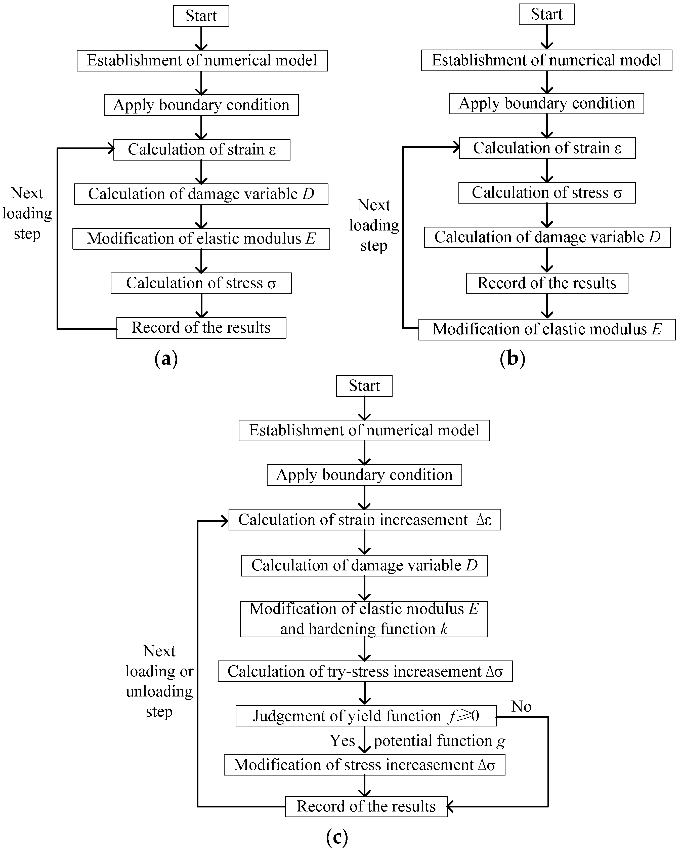
3.3. Damage Calculation Programs

The original constitutive relations need to be revised so that the effect of damage can be introduced. Based on different models, the corresponding algorithms were developed, respectively, as shown in Figure 3. Furthermore, the modification of the elastic modulus and the updating of the calculation results due to damage are integrated into the original FEM software by adding some codes or programs.

4. Results and Discussion

4.1. Uniform Compression Condition

4.1.1. Stress-Strain Response

Stress-strain curves were often used to describe the deformation and failure process of rock specimens. In this section, the test results [47,48] were used for verification. Three models were calculated respectively under the boundary conditions in which the top and bottom surfaces were set free in the horizontal direction. The results of the stress-strain curves are illustrated in Figure 4. The horizontal axis represents the axial strain obtained by the ratio of the given axial displacement to the model height. The vertical axis represents the axial stress obtained by the ratio of the stress integral on the top surface to its area.

Most test curves can be divided into the initial compaction stage, elastic deformation stage, hardening stage, post-peak softening stage, and residual stage [49]. The curves obtained from three damage models are all in good agreement with the experimental data in the pre-peak stage. However, in the post-peak stage, a large deviation between the curve of the empirical model and the test curve is observed. It can be concluded that the statistical damage model and elastoplastic damage model are better for simulating the stress-strain curve of samples under uniform compression conditions.

4.1.2. Damage Distribution and Evolution

In most previous studies, whether the stress-strain curve can be verified was regarded as a reasonable standard. However, the distribution and evolution of damage and deformation inside are of importance in the rock failure process. Therefore, only validating the stress-strain curves is not adequate for the evaluation of a damage model. The damage distribution and evolution of different models are plotted in Figure 5. The deformation is magnified 10 times for better display.

Figure 5 shows that there is only one damage value in the whole sample at a certain time, which means that the damage distribution inside the three samples was uniform. The value of the damage variable rises with the increase of axial displacement. The maximum value of the damage variables in all three models can almost be close to 1.0. In the empirical damage model, the damage variable is related to axial strain, and thus damage emerges at the beginning of compression and develops gradually. In the statistical damage model, damage occurs when the yield point has been reached according to the adopted yield criterion. In the elastoplastic damage model, the damage variable is associated with volumetric strain, and thus damage occurs when the volume begins to inflate. According to different damage mechanisms, the corresponding definition of the damage variable should be expected.

4.2. Nonuniform Stress Condition

4.2.1. Stress-Strain Response

The uniform compression condition discussed in Section 4.1 is rarely encountered in reality. Rocks in engineering always faced ununiform stress conditions and even severe stress concentrations. The boundary of setting the top and bottom faces to be fixed in the horizontal direction was adopted to simulate the ununiform stress condition. The obtained stress-strain curves are plotted in Figure 6.

The results of the empirical and statistical damage models under ununiform stress conditions are quite different from those under uniform forced conditions. The complete stress-strain curve can be obtained and matches test curves well under uniform stress condition. However, only the pre-peak stage can be obtained under ununiform stress conditions. The empirical damage model can only be calculated until the axial strain reaches 0.0021. The calculation of the statistical damage model stops once the axial strain reaches 0.0023. The elastoplastic damage model can give the post-peak stage of the stress-strain curves and match test data well. The results show that in the first two damage models, the stress-strain curves suddenly drop before the peak stress rather than passing the peak stress. The reason is that the compulsory reduction of the elastic modulus can probably lead to extreme element distortion where the stress is concentrated, which inevitably causes the numerical simulation to fail prematurely. As to the elastoplastic damage model, it also achieved the strain-softening stage, and the difference in the stress-strain curves was reflected in the residual strength rather than the peak strength. Therefore, the elastoplastic damage models are more appropriate for describing the damage and failure process by numerically simulating with FEM. It should also be pointed out that the treatment of the adverse effect of local deterioration due to damage is the important issue in numerical simulations.

4.2.2. Damage Distribution and Evolution

The damage distribution and evolution under nonuniform stress conditions are discussed in this section. The results are plotted in Figure 7. The deformation is also magnified 10 times for better display.

As can be seen from Figure 7, the damage distribution inside samples was not uniform. The empirical and statistical damage model can only be calculated until the axial strain reaches 0.0023 and 0.0021, respectively. Since the top and bottom surfaces are fixed in a horizontal direction, stress concentration appears at the corners of top and bottom surfaces. Because the damage variables are related to the strain and stress states directly, maximum values of more than 0.90 have emerged in these zones of stress concentration, while damage variables inside the samples are still almost zero. The severe damage due stress concentration leads to the serious distortion of some elements at the corners of top and bottom surfaces, which inevitably causes the calculation of the whole model to be terminated. In the elastoplastic damage model, damage was supposed to occur when the volume begins to inflate. Although stress concentration emerges at the corners of top and bottom surfaces, the inflated volumetric strain appears near the middle cylindrical surface of the sample first. Therefore, the damage distributes mainly in the middle sample but not on the corner of end surfaces. After the axial strain reaches 0.0045, the middle part of sample has inflated heavily and causes the fatal distortion of some elements that terminates the whole calculation. This is the reason why the elastoplastic damage model can be calculated continuously in spite of stress concentration at the corners of end surfaces.

4.3. Discussion

As discussed above, the empirical damage model and statistical damage model are deduced based on generalized Hooke’s law and only consider damage-elastic coupling. The models can describe the stress-strain behaviors under uniform compression conditions well but fail to give complete curves under ununiform stress conditions. The irreversible damage deformation cannot be derived due to the limits of the damage variable definition and current FEM software. The elastoplastic damage model was established by considering the damage-elastic-plastic coupling mechanism. It can be adopted to describe the whole stress-strain behavior and the irreversible damage evolution under both conditions well.

The continuum damage models were established by examining the overall macroscopic response of the sample. The analysis basis is the macroscopic mechanical behaviors of specimens that are influenced by all damage inside the specimens. The kinds of mode parameters are obtained by a whole specimen. Although the statistical damage model is built based on the probability distribution of microscopic units inside the sample, the final derived damage variable is expressed as an overall deterioration value of the whole specimen’s properties through mathematical methods ingeniously. It is different from some mesoscopic numerical simulation software in which the internal heterogeneous properties are truly distributed; the statistical damage model is just a mathematical method that gives a self-consistent result in theory. When applying these continuum damage models into FEM calculations, every element is considered as a whole specimen according to the definition of macroscopical damage variables. Some local severe damages can result in the termination of the calculation, although these damages are distributed only in very tiny zones that should not affect the overall bearing capacity. It can be inferred that a more reasonable definition of damage variables should represent the local effect of damage and be tracked during the whole deformation and failure process.

In fact, rock is a special material that has a lot of defects. Damage often occurs near the defect first. However, many damage models, such as the empirical and statistical damage models mentioned above, regard the sample as a whole, and thus they can give some macroscopic response characteristics of the sample but cannot describe the internal damage distribution and evolution well. Therefore, more and more experts conducted discussions on the problem of damage localization [3,50]. Some professors put forward novel ideas, such as the failure approach index [51] and the phase-field method [52], to better study the damage evolution and distribution.

5. Conclusions

The continuum damage models are grouped into empirical damage models, statistical damage models, and elastoplastic damage models. Three representative models were studied by numerical simulations with self-developed programs. The conclusions were drawn as follows.

(1)

The empirical damage models and statistical damage models considering damage-elastic coupling can present strain-softening stages under uniform compression conditions. Such a descent of a stress-strain curve is caused by subtracting elastic modulus gradually, which cannot reflect the irreversibility of the damage well.

(2)

The elastoplastic damage models considering the damage-elastic-plastic coupling can present strain-softening stages under both uniform compression conditions and ununiform stress conditions. Such a descent of a stress-strain curve is caused by reducing plastic yield stress gradually, which can represent the irreversibility of damage.

(3)

Every element in FEM simulations is considered as a whole specimen, as indicated by the continuum damage models. The compulsory reduction of the elastic modulus can probably lead to extreme element distortion and even an unreasonable negative modulus when the damage of an element is very serious, and therefore prematurely result in the failure of overall numerical simulations under complex stress states.

(4)

The internal damage distribution and evolution can be obtained according to the specific damage definitions, which reveals the different damage mechanisms. The most reasonable definition of the damage variable should be expected to reflect the local deterioration effect and irreversibility feature of damage.

References

1. Liu, X.; Kou, M.; Lu, Y.; Liu, Y. An Experimental Investigation on the Shear Mechanism of Fatigue Damage in Rock Joints under Pre-peak Cyclic Loading Condition. Int. J. Fatigue 2018, 106, 175–184. [Google Scholar] [CrossRef]
2. Tang, C.; Liu, H.; Lee, P.; Tsui, Y.; Tham, L. Numerical Studies of the Influence of Microstructure on Rock Failure in Uniaxial Compression-Part I: Effect of Heterogeneity. Int. J. Rock Mech. Min. Sci. 2000, 37, 555–569. [Google Scholar] [CrossRef]
3. Xu, X.; Ma, S.; Xia, M.; Ke, F.; Bai, Y. Damage Evaluation and Damage Localization of Rock. Theor. Appl. Fract. Mech. 2004, 42, 131–138. [Google Scholar] [CrossRef]
4. Peng, R.; Ju, Y.; Wang, J.; Xie, H.; Gao, F.; Mao, L. Energy Dissipation and Release During Coal Failure Under Conventional Triaxial Compression. Rock Mech. Rock Eng. 2014, 48, 509–526. [Google Scholar] [CrossRef]
5. Ahmed, Z.; Wang, S.; Hashmi, M.Z.; Zishan, Z.; Chengjin, Z. Causes, characterization, damage models, and constitutive modes for rock damage analysis: A review. Arab. J. Geosci. 2020, 13, 806. [Google Scholar] [CrossRef]
6. Zhang, J.; Ma, L.; Zhang, Z.X. Elastoplastic Damage Model for Concrete Under Triaxial Compression and Reversed Cyclic Loading. Strength Mater. 2018, 50, 724–734. [Google Scholar] [CrossRef]
7. Lemaitre, J. How to Use Damage Mechanics. Nucl. Eng. Des. 1984, 80, 233–245. [Google Scholar] [CrossRef]
8. Rabotnov, Y.N. On the Equations of State for Creep. Proc. Inst. Mech. Eng. Conf. Proc. 1963, 178, 2–117. [Google Scholar] [CrossRef]
9. Davison, L.; Stevens, A.L. Thermomechanical Constitution of Spalling Elastic Bodies. J. Appl. Phys. 1973, 44, 668–674. [Google Scholar] [CrossRef]
10. Gurson, A.L. Continuum Theory of Ductile Rupture by Void Nucleation and Growth. Part I. Yield Criteria and Flow Rules for Porous Ductile Media. J. Eng. Mater. Tech. 1977, 4, 2–15. [Google Scholar] [CrossRef]
11. Dragon, A.; Mróz, Z. Continuum Model for Plastic-brittle Behavior of Rock and Concrete. Int. J. Eng. Sci. 1979, 17, 121–137. [Google Scholar] [CrossRef]
12. Chaboche, J.L. Anisotropic Creep Damage in the Framework of Continuum Damage Mechanics. Nucl. Eng. Des. 1984, 79, 309–319. [Google Scholar] [CrossRef]
13. Jansson, S.; Stigh, U. Influence of Cavity Shape on Damage Parameter. J. Appl. Mech. 1985, 52, 609–614. [Google Scholar] [CrossRef]
14. Ju, Y.; Xie, H.P. Applicability of Damage Variable Definition Based on Hypothesis of Strain Equivalence. J. Coal Sci. Eng. 2000, 6, 9–14. [Google Scholar]
15. Deng, J.; Gu, D. On a Statistical Damage Constitutive Model for Rock Materials. Comput. Geosci. 2011, 37, 122–128. [Google Scholar] [CrossRef]
16. Løland, K. Continuous Damage Model for Load-response Estimation of Concrete. Cem. Concr. Res. 1980, 10, 395–402. [Google Scholar] [CrossRef]
17. Mazars, J.; Pijaudier-Cabot, G. Continuum Damage Theory-Application to Concrete. J. Eng. Mech. 1989, 115, 345–365. [Google Scholar] [CrossRef]
18. Xie, H.P.; Ju, Y. A Study of Damage Mechanics Theory in Fractional Dimensional Space. Chin. J. Rock Mech. Eng. 1999, 31, 300–310. (In Chinese) [Google Scholar]
19. Shen, P.; Tang, H.; Wang, D.; Ning, Y.; Zhang, Y.; Su, X. A Statistical Damage Constitutive Model Based on Unified Strength Theory for Embankment Rocks. Mar. Georesources Geotechnol. 2019, 38, 818–829. [Google Scholar] [CrossRef]
20. Bruning, T.; Karakus, M.; Nguyen, G.; Goodchild, D. An Experimental and Theoretical Stress-strain-damage Correlation Procedure for Constitutive Modelling of Granite. Int. J. Rock Mech. Min. Sci. 2019, 116, 1–12. [Google Scholar] [CrossRef]
21. Huang, X.; Kong, X.; Chen, Z.; Fang, Q. A plastic-damage model for rock-like materials focused on damage mechanisms under high pressure. Comput. Geotech. 2021, 137, 104263. [Google Scholar] [CrossRef]
22. Chang, S.-H.; Lee, C.-I.; Lee, Y.-K. An experimental damage model and its application to the evaluation of the excavation damage zone. Rock Mech. Rock Eng. 2007, 40, 245–285. [Google Scholar] [CrossRef]
23. Zhao, G.; Chen, C.; Yan, H.; Hao, Y. Study on the damage characteristics and damage model of organic rock oil shale under the temperature effect. Arab. J. Geosci. 2021, 14, 722. [Google Scholar] [CrossRef]
24. Zhu, Z.; Tian, H.; Wang, R.; Jiang, G.; Dou, B.; Mei, G. Statistical thermal damage constitutive model of rocks based on Weibull distribution. Arab. J. Geosci. 2021, 14, 495. [Google Scholar] [CrossRef]
25. Salari, M.; Saeb, S.; Willam, K.; Patchet, S.; Carrasco, R. A Coupled Elastoplastic Damage Model for Geomaterials. Comput. Methods Appl. Mech. Eng. 2004, 193, 2625–2643. [Google Scholar] [CrossRef]
26. Chen, L.; Shao, J.; Huang, H. Coupled Elastoplastic Damage Modeling of Anisotropic Rocks. Comput. Geotech. 2009, 37, 187–194. [Google Scholar] [CrossRef]
27. Richard, B.; Ragueneau, F. Continuum Damage Mechanics Based Model for Quasi Brittle Materials Subjected to Cyclic Loadings: Formulation, Numerical Implementation, and Applications. Eng. Fract. Mech. 2013, 98, 383–406. [Google Scholar] [CrossRef]
28. Liu, X.M.; Li, C.F. Damage Mechanics Analysis for Brittle Rock and Rockbust Energy Index. Chin. J. Rock Mech. Eng. 1997, 16, 45–52. (In Chinese) [Google Scholar]
29. Yan, X.; Jun, L.; Yijin, Z.; Shidong, D.; Tingxue, J. Research on Lateral Scale Effect and Constitutive Model of Rock Damage Energy Evolution. Geotech. Geol. Eng. 2018, 36, 2415–2424. [Google Scholar] [CrossRef]
30. Liu, X.; Ning, J.; Tan, Y.; Gu, Q. Damage constitutive model based on energy dissipation for intact rock subjected to cyclic loading. Int. J. Rock Mech. Min. Sci. 2016, 85, 27–32. [Google Scholar] [CrossRef]
31. Chen, X.; He, P.; Qin, Z.; Li, J.; Gong, Y. Statistical Damage Model of Altered Granite under Dry-Wet Cycles. Symmetry 2019, 11, 41. [Google Scholar] [CrossRef]
32. Zhao, H.; Zhou, S.; Zhang, L. A phenomenological modeling of rocks based on the influence of damage initiation. Environ. Earth Sci. 2019, 78, 143. [Google Scholar] [CrossRef]
33. Jiang, H.; Li, K.; Hou, X. Statistical damage model of rocks reflecting strain softening considering the influences of both damage threshold and residual strength. Arab. J. Geosci. 2020, 13, 286. [Google Scholar] [CrossRef]
34. Yang, J.P.; Chen, W.Z.; Huang, S. Study of A Statistic Damage Constitutive Model for Rocks. Rock Soil Mech. 2010, 31, 7–11. (In Chinese) [Google Scholar]
35. Liu, W.; Zhang, S.; Sun, B. Energy Evolution of Rock under Different Stress Paths and Establishment of a Statistical Damage Model. KSCE J. Civ. Eng. 2019, 23, 4274–4287. [Google Scholar] [CrossRef]
36. Wang, Z.L.; Li, Y.C.; Wang, J. A Damage-softening Statistical Constitutive Model Considering Rock Residual Strength. Comput. Geosci. 2007, 33, 1–9. [Google Scholar] [CrossRef]
37. Cai, W.; Dou, L.; Ju, Y.; Cao, W.; Yuan, S.; Si, G. A Plastic Strain-based Damage Model for Heterogeneous Coal using Cohesion and Dilation Angle. Int. J. Rock Mech. Min. Sci. 2018, 110, 151–160. [Google Scholar] [CrossRef]
38. Han, Y.-F.; Cheng, X.-Y.; Liu, X.-R.; Zhao, L.-L.; He, J.; Miao, J. Extraction and Numerical Simulation of Gas-water Flow in Low Permeability Coal Reservoirs Based on a Pore Network Model. Energy Sources Part A Recover. Util. Environ. Eff. 2019, 43, 1945–1957. [Google Scholar] [CrossRef]
39. Zhang, H.; Meng, X.; Liu, X. Establishment of constitutive model and analysis of damage characteristics of frozen-thawed rock under load. Arab. J. Geosci. 2021, 14, 1277. [Google Scholar] [CrossRef]
40. Liu, Y.; Dai, F. A damage constitutive model for intermittent jointed rocks under cyclic uniaxial compression. Int. J. Rock Mech. Min. Sci. 2018, 103, 289–301. [Google Scholar] [CrossRef]
41. Zhou, S.W.; Xia, C.C.; Zhao, H.B.; Mei, S.-H.; Zhou, Y. Statistical Damage Constitutive Model for Rocks Subjected to Cyclic Stress and Cyclic Temperature. Acta Geophys. 2017, 65, 893–906. [Google Scholar] [CrossRef]
42. Fan, X.; Luo, N.; Yuan, Y.; Liang, H.; Zhai, C.; Qu, Z.; Li, M. Dynamic mechanical behavior and damage constitutive model of shales with different bedding under compressive impact loading. Arab. J. Geosci. 2021, 14, 1752. [Google Scholar] [CrossRef]
43. Wang, C.; Zhan, S.F.; Xie, M.Z.; Wang, C.; Cheng, L.-P.; Xiong, Z.-Q. Damage Characteristics and Constitutive Model of Deep Rock under Frequent Impact Disturbances in the Process of Unloading High Static Stress. Complexity 2020, 2020, 2706091. [Google Scholar] [CrossRef]
44. Tu, X.; Andrade, J.E.; Chen, Q. Return mapping for nonsmooth and multiscale elastoplasticity. Comput. Methods Appl. Mech. Eng. 2009, 198, 2286–2296. [Google Scholar] [CrossRef]
45. Yuan, X.P.; Liu, H.Y.; Wang, Z.Q. Study of Elastoplastic Damage Constitutive Model of Rocks Based on Drucker-Prager Criterion. Rock Soil Mech. 2012, 33, 1103–1108. (In Chinese) [Google Scholar]
46. Borja, R.I.; Sama, K.M.; Sanz, P.F. On the numerical integration of three-invariant elastoplastic constitutive models. Comput. Methods Appl. Mech. Eng. 2003, 192, 1227–1258. [Google Scholar] [CrossRef]
47. Li, X.; Cao, W.-G.; Su, Y.-H. A Statistical Damage Constitutive Model for Softening Behavior of Rocks. Eng. Geol. 2012, 143–144, 1–17. [Google Scholar] [CrossRef]
48. Rummel, F.; Fairhurst, C. Determination of the post-failure behavior of brittle rock using a servo-controlled testing machine. Rock Mech. Rock Eng. 1970, 2, 189–204. [Google Scholar] [CrossRef]
49. Chen, Y.; Zuo, J.; Li, Z.; Dou, R. Experimental Investigation on the Crack Propagation Behaviors of Sandstone under Different Loading and Unloading Conditions. Int. J. Rock Mech. Min. Sci. 2020, 130, 104310. [Google Scholar] [CrossRef]
50. Gao, M.; Liang, Z.; Li, Y.; Wu, X.; Zhang, M. End and Shape Effects of Brittle Rock under Uniaxial Compression. Arab. J. Geosci. 2018, 11, 614. [Google Scholar] [CrossRef]
51. Zhang, N.-H.; Wang, J.-J.; Cheng, C.-J. Stability Assessment of Rockmass Engineering Based on Failure Approach Index. Appl. Math. Mech. 2007, 28, 888–894. (In Chinese) [Google Scholar] [CrossRef]
52. Ambati, M.; Gerasimov, T.; De Lorenzis, L. A Review on Phase-field Models of Brittle Fracture and a New Fast Hybrid Formulation. Comput. Mech. 2014, 55, 383–405. [Google Scholar] [CrossRef]
Figure 1. Calculating principle of damage models: (a) the empirical damage model; (b) the statistical damage model; and (c) the elastoplastic damage model.
Energies 15 06806 g001
Figure 2. Schematics of boundary conditions for uniaxial compression: (a) an ideal case with a free end; (b) an extreme case with a fixed end.
Energies 15 06806 g002
Figure 3. Calculation programs of three representative models: (a) the empirical damage model; (b) the statistical damage model; and (c) the elastoplastic damage model.
Energies 15 06806 g003
Figure 4. Stress–strain curves under uniform compression conditions.
Energies 15 06806 g004
Figure 5. The damage distribution and evolution of different models under uniform compression conditions: (a) the empirical damage model; (b) the statistical damage model; and (c) the elasto–plastic damage model.
Energies 15 06806 g005aEnergies 15 06806 g005b
Figure 6. Stress–strain curves under ununiform stress condition.
Energies 15 06806 g006
Figure 7. The damage distribution and evolution of different models under ununiform stress con–ditions: (a) the empirical damage model; (b) the statistical damage model; and (c) the elastoplastic damage model.
Energies 15 06806 g007aEnergies 15 06806 g007b