A Particle-Scale Model of Surface Tension for Two-Phase Flow: Model Description and Validation

Abstract

A particle-scale surface tension force model (STF) is proposed here to be incorporated in the smoothed hydrodynamics particle (SPH) method. This model is based on the identification of interface geometry and the gradient of densities across the interface. A square bubble of single-phase and a square bubble immersed in fluids are simulated by the STF model accompanied with a combined kernel in SPH to validate their suitability to simulate the immersed bubble motion. Two cases of rising bubbles, i.e., a single rising bubble and a pair of rising bubbles, are simulated for demonstration. The rising velocity, density, surface tension force, interfacial curvature, the power of the STF, and the smoothing length of the rising bubble and surrounding fluids are all computed by the current STF model to study the characteristics of immersed bubble’s motion and coalescence. The current model provides a way to capture the interfacial interactions in two-phase flows at particle scales.

1. Introduction

The interfacial phenomenon with thin liquid films [1] or free surfaces [2] in two-phase flows is always important and complex in many engineering processes. For example, the critical heat flux in the boiling process is important in understanding and predicting the heat transfer issues in the reactor thermal hydraulics. In particular, the surface tension force (STF) is a fundamental issue in two-phase flows, especially when we need to capture the phase change dynamics. To tackle STF in simulating two-phase flows, usually based on the continuous surface force description, one always needs to know the local normal vector on the interface and the curvature on that point.

In computational fluid dynamics, the most common methods to solve the surface tension forces are the volume of fluid method (VOF) [3], the level set method (LS) [4], and the front tracking method [5]. The main shortcoming of these methods lays in the prediction of the evolution of a moving interface [6], which may, in turn, cause the methods to fail in accurately predicting the accurate normal direction and curvature on the surface [7]. Therefore, many choices have been considered and developed, such as the moving particle semi-implicit (MPS) method [8], the dissipative particle dynamics (DPD) method [9], and the smoothed particle hydrodynamics method [10]. The smoothed particle hydrodynamics (SPH) is considered a meshfree, Lagrangian, particle method, which is advantageous over conventional grid-based numerical methods in the aspect of interface treatment [11].

In general, surface tension is a force at the interface of two kinds of fluids or one kind of fluid with differential densities. The STF is explained at the molecular level by an imbalance of the interactions between the molecules of the two fluids [12]. Although the STF is a surface force that depends on the local normal direction of the surface and the local curvature of the surface, it is always simplified by volumetric expressions to be incorporated in the continuous surface force model (CSF) [13] or Continuum Stress Surface (CSS) method [14]. In addition, there is another way to compute the surface tension force, i.e., by imposing additional forces on particles to mimic the local imbalance between particles on the interface. These additional forces are usually pair-wise forces to mimic the imbalance of molecular interactions [15]. Although this method is particularly suitable for particle-based methods (or from the Lagrangian viewpoint of description), e.g., the smoothed particle hydrodynamics method, it does need substantial research on calibration and may be case-dependent or material-varied expressions on particle–particle interactions should be utilized. As a key issue, how to mimic the particle-scale imbalance on the interface which is generated from the imbalance of molecules is difficult since the scales may vary over several orders.

In this work, a particle-scale surface tension force model is proposed based on particle-scale computations of the local normal force by the gradient of densities and local curvature of a one- or two-layer interfacial surface. This method is based on the smoothed particle hydrodynamics method and three validation cases and two demonstrative application cases have been carried out. However, we believe that this method can be utilized in common cases of two-phase flows.

2. Mathematical Formulations

2.1. Governing Equations for SPH

For the fluids with properties of density $\rho$, velocity $v$, pressure p, and viscosity $\mu$, the governing equations are the Navier–Stokes equations formulated as follows

$$\begin{array}{c}\hfill \begin{array}{cc}& \frac{d\rho }{dt}=-\rho \nabla ·v\hfill \\ & \frac{dv}{dt}=-\frac{1}{\rho }\nabla p+\frac{1}{\rho }\nabla ·\tau +f_{ext}\hfill \end{array}\end{array}$$

(1)

The deviator stress tensor $\tau$ is usually expressed by

$$\begin{array}{c}\hfill \begin{array}{c}\hfill \tau =\mu ϵ=\mu \left(\nabla v+\nabla v^T-\frac{2}{3}(\nabla ·v){\delta }_{\alpha \beta }\right)\end{array}\end{array}$$

(2)

where ${\delta }_{\alpha \beta }$

$$\begin{array}{c}\hfill \begin{array}{c}\hfill {\delta }_{\alpha \beta }=\left\{\begin{array}{c}1,\mathrm{if}\alpha =\beta \hfill \\ 0,\mathrm{otherwise}\hfill \end{array}\right.\end{array}\end{array}$$

(3)

is the Kronecker delta function. $f_{ext}$ is the total external force field which may normally include the forces of gravity $f_G$, buoyancy $f_B$, surface tension $f_S$, etc.

In smoothed particle hydrodynamics, the quantities and their derivatives are always discretized by using suitable kernel functions ($W_{ij}\left(r\right)$) to cope with particle–particle interactions, where $r=|x_i-x_j|$ and $x_i$ is the position vector of the ith particle. The quantities are usually the density ${\rho }^a$, pressure $p^a$, etc., (hereafter a = $\left(l\right)iquid$, $\left(g\right)as$, which means the index of phases in liquid-gas two-phase flow; and the superscript can always be omitted if it does not make confusion). Based on the kernel function, the smoothed particle hydrodynamics formulates the Navier–Stokes equations of continuous fluid flow as follows

$$\begin{array}{c}\hfill \begin{array}{cc}\hfill \frac{d{\rho }_i}{dt}& ={\rho }_i\sum _{j=1}^N\frac{m_j}{{\rho }_j}{\left(v_{ij}\right)}_{\beta }·{\nabla }_{i,\beta }{W}_{ij}\hfill \\ \hfill \frac{d{\left(v_i\right)}_{\alpha }}{dt}& =\sum _{j=1}^N{m}_j\left(\frac{-p_i{I}_{\alpha \beta }+{\mu }_i{\left({ϵ}_i\right)}_{\alpha \beta }}{{\rho }_i^2}+\frac{-p_j{I}_{\alpha \beta }+{\mu }_j{\left({ϵ}_j\right)}_{\alpha \beta }}{{\rho }_j^2}\right)·{\nabla }_{i,\beta }{W}_{ij}\hfill \\ & +{\left(f_{Gi}\right)}_{\alpha }+{\left(f_{Bi}\right)}_{\alpha }+{\left(f_{Si}\right)}_{\alpha }\hfill \end{array}\end{array}$$

(4)

where $\alpha ,\beta =(x,y,z)$. $m_i$, ${\rho }_i$, $p_i$, $v_i$ are mass, density, pressure, and velocity of the ith particle. $v_i=v_i-v_j$ is the velocity difference between the ith and jth particle. $I$ is the identity matrix and ∇ is the gradient operator. The strain rate tensor ${\left({ϵ}_i\right)}_{\alpha \beta }$ is

$$\begin{array}{c}\hfill \begin{array}{cc}\hfill {(ϵ}_i{)}_{\alpha \beta }& =\sum _{j=1}^N\frac{m_j}{{\rho }_j}\left({\left(v_{ji}\right)}_{\alpha }{\nabla }_{i,\beta }{W}_{ij}+{\left(v_{ji}\right)}_{\beta }{\nabla }_{i,\alpha }{W}_{ij}-\frac{2}{3}{\delta }_{\alpha \beta }{v}_{ji}·{\nabla }_i{W}_{ij}\right)\hfill \end{array}\end{array}$$

(5)

In two-phase flow, the gravity term $f_{Gi}$, the buoyant force term $f_{Bi}$ are respectively expressed as follows

$$\begin{array}{c}\hfill \begin{array}{cc}\hfill f_{Gi}& =g\hfill \\ \hfill f_{Bi}& =-\left(\frac{{\rho }_l-{\rho }_i}{{\rho }_l}\right)g\hfill \end{array}\end{array}$$

(6)

The inter-phase interaction force term $f_{Si}$ is considered as the surface tension force here [16]

$$\begin{array}{c}\hfill \begin{array}{c}\hfill f_{Si}=2{\delta }_{Si}\sigma {\kappa }_i{n}_i\end{array}\end{array}$$

(7)

where $\sigma$ is the surface tension coefficient. ${\kappa }_i$ and $n_i$ are the local mean interface curvature and unit normal vector at $x_i$, respectively. ${\delta }_{Si}$ is a function that determines if it is the interface between two phases.

In addition, the equation of state used here follows the formulation of [12]:

$$\begin{array}{c}\hfill p_e\left({\rho }_i\right)=p_r\left({\left(\frac{\rho }{{\rho }_0}\right)}^{\gamma }-1\right)+p_0\end{array}$$

(8)

where ${\rho }_0$ is the constant reference density for fluid particles, and $p_r$ and $p_0$ are the reference pressure and background pressure of the fluid, respectively.

Concerning the kernel function, herein, we used a newly self-developed kernel function. Suppose r is the distance between any pair of particles, and h is the smoothing length, the kernel function is

$$\begin{array}{c}\hfill W\left(r,h\right)={\alpha }_D\left\{\begin{array}{c}\frac{h}{r}+{\left(3-\frac{r}{h}\right)}^3,0<r\le 2\hfill \\ 0,r>2\hfill \end{array}\right.\end{array}$$

(9)

where the coefficient ${\alpha }_D$ is to take the integral of the kernel over any local domain $\Omega$ of cut-radius $R_c$ to be unity. For example, in a 2D case, it should satisfy

$$\begin{array}{c}\hfill \begin{array}{c}\hfill {\int }_{\Omega }W\left(r,h\right)d\Omega ={\int }_0^{2\pi }{\int }_0^{R_c}W(r,h)=1,\end{array}\end{array}$$

(10)

and get ${\alpha }_D=\frac{5}{136\pi h^2}$.

2.2. Particle-Scale Surface Tension Force

As aforementioned, existing methods for surface tension force in SPH may generally be divided into three categories, e.g., using cohesive pressures [17], inter-particle forces [18], and continuum surface forces [13]. In this work, the surface tension force formulation is based on Equation (7). So, it is still within the category of the continuum surface force model. However, the implemented schemes are different.

In Equation (7), there are three issues to be addressed in detail: (1) an index function ${\delta }_{Si}$ which determines where is the inter-phase or free surface. (2) The normal vector $n_i$ on the free surface or inter-phase surface where the ith particle is located; (3) the geometric curvature ${\kappa }_i$ of the local interface.

For the index function, it is easy to be implemented numerically in SPH. For example, we can determine the interface by

$$\begin{array}{c}\hfill \begin{array}{c}\hfill {\delta }_S\left(x\right)=|x_i^l-x_j^g|<ch\end{array}\end{array}$$

(11)

which means that the distance between the ith liquid particle and the jth gas particle is less than $ch$. Herein, h is the smoothing/interaction distance in SPH, and c is a tuned coefficient. In general, we let $c=1$ here to avoid tuning the coefficient.

In the existing literature [7,12], the normal vector of the inter-phase is always computed by a scalar function $c(x,y)$ which is the volumetric or number density of the liquid (or gas) phase. The idea of using the scale function c (or color function) is somewhat like the level-set method or VOF method [11], where the normal vector of the surface is the gradient of the scalar function, i.e., $n=\frac{\nabla c}{|\nabla c|}$, and the curvature given by $\kappa =\nabla ·n$. Using this concept, the gradient cannot be very sharp due to the requirement to maintain stability in numerical implementations.

However, we scrutinized this method and finally gave up using the scalar function $c(x,y)$. Instead, based on the index function of Equation (11), we think that it is suitable to be reformed as follows:

$$\begin{array}{c}\hfill \begin{array}{c}\hfill {\delta }_S\left(x\right)=|x_i^l-x_j^g|={\delta }_S\left(s_{ij}\right)\end{array}\end{array}$$

(12)

As ${\delta }_S$ is known in the first step (Equation 11), if we generate a group of functions $\left(g_{I\alpha }\right):{\delta }_S\to R^1$ on ${\delta }_S\left(s_{ij}\right)$, after some labor, it is easy to derive the tangential vector ${\tau }_s$ and the magnitude of the unit normal vector $n_s^0$, respectively, by

$$\begin{array}{c}\hfill \begin{array}{cc}\hfill {\left({\tau }_s\right)}_{\alpha }& =\frac{d{g}_{I\alpha }}{ds}\hfill \\ \hfill \left|\right|n_s|{|}_{\alpha }^0& =\frac{1}{\left|\right|\frac{d^2{g}_{I\alpha }\left(s\right)}{d{s}^2}\left|\right|}||\frac{d^2{g}_{I\alpha }}{d{s}^2}||\hfill \end{array}\end{array}$$

(13)

As the normal vector magnitude has already been obtained by Equation (13), one needs only to determine the correct direction of it, i.e., either $n_s$ or $-n_s$. Then, the gradient of the density of fluid $\nabla \rho$ is used to aid to determine the correct direction of the surface tension force, i.e.,

$$\begin{array}{c}\hfill \begin{array}{c}\hfill n_s=\left\{\begin{array}{c}{n}_s,\mathrm{if}\nabla \rho ·n_s\ge 0\hfill \\ -n_s,\mathrm{if}\nabla \rho ·n_s<0\hfill \end{array}\right.\end{array}\end{array}$$

(14)

The gradient of the density of the jth particle is obtained by

$$\begin{array}{c}\hfill \begin{array}{c}\hfill \nabla {\rho }_j=\sum _{(i,j)\in {\Sigma }_{inf}}(x_i-x_j)({\rho }_j-{\rho }_i)\end{array}\end{array}$$

(15)

where $(i,j)\in {\Sigma }_{inf}$ means either the ith or the jth particle is on the two-phase interface ${\Sigma }_{inf}$.

In addition, the curvature can be directly obtained by Equation (13), i.e.,

$$\begin{array}{c}\hfill \begin{array}{c}\hfill \kappa ={\left[\sum {\left(\frac{d^2{g}_{I\alpha }\left(s\right)}{d{s}^2}\right)}^2\right]}^{1/2}\end{array}\end{array}$$

(16)

Note that Equations (13) and (16) give respectively the unit normal vector and curvature in Equation (16). Its accuracy is mainly determined by the interface index function ${\delta }_S$ given by Equation (11). As the interface function is, for example, a one-dimensional curve in two-dimensional two-phase flows, it could be maintained very sharp and accurate with some regression or smoothing techniques. In other words, its accuracy may be maintained ideally as high as required.

Using the current particle-scale model, the surface tension forces can be computed on the interface of an internal bubble and surrounding fluids (Figure 1). In this work, although the coefficient $c=1$ in Equation (11) is used, the smoothing length h is determined by the densities on each side of the interface. Therefore, in Figure 1, the surface tension force is computed on two layers of the fluid particles (high density, red particle), whereas it is only computed on one layer of the bubble particle (lower density, blue particle). We think that the interface treated in this method is as thin as possible to take only one or two particles on both sides. We may call this method a particle-scale model of the surface tension force.

3. Validations and Results

3.1. Validation Case 1 for the Kernel: Dam-Break

As a first step, this section shows the validation for the kernel proposed here. A dam-break case is chosen herein which is simulated by using the current kernel (Equation (9)) and the results are compared to existing simulations [19,20,21] and experiments [22]. The dam-break case occurs in a wet bed of 9.55 m length in the water depth of $h_d=0.038$ m. Before the dam-break, the waters on the left side of the bed are 0.38 m and 0.15 m in width and height, respectively. A total of 32,022 particles were used to simulate this case.

The water waves and profiles at time step t = 0.28, 0.34, and 0.47 s are shown in Figure 2a–c, respectively, accompanied with existing numerical and experimental counterparts [19,20,21,22]. It is seen that the current results have a few differences from the experimental results [22]. In addition, there are similar differences between the existing simulation results and experimental results. However, the consistency between the current simulation and existing numerical results [19,20,21] seems to be acceptable. To say conclusively, the profiles obtained by numerical simulations with different kernels look more or less consistent with each other. This indicates that the current kernel is suitable and capable of simulating the fluid flows. Hence, we will use this kernel for subsequent cases.

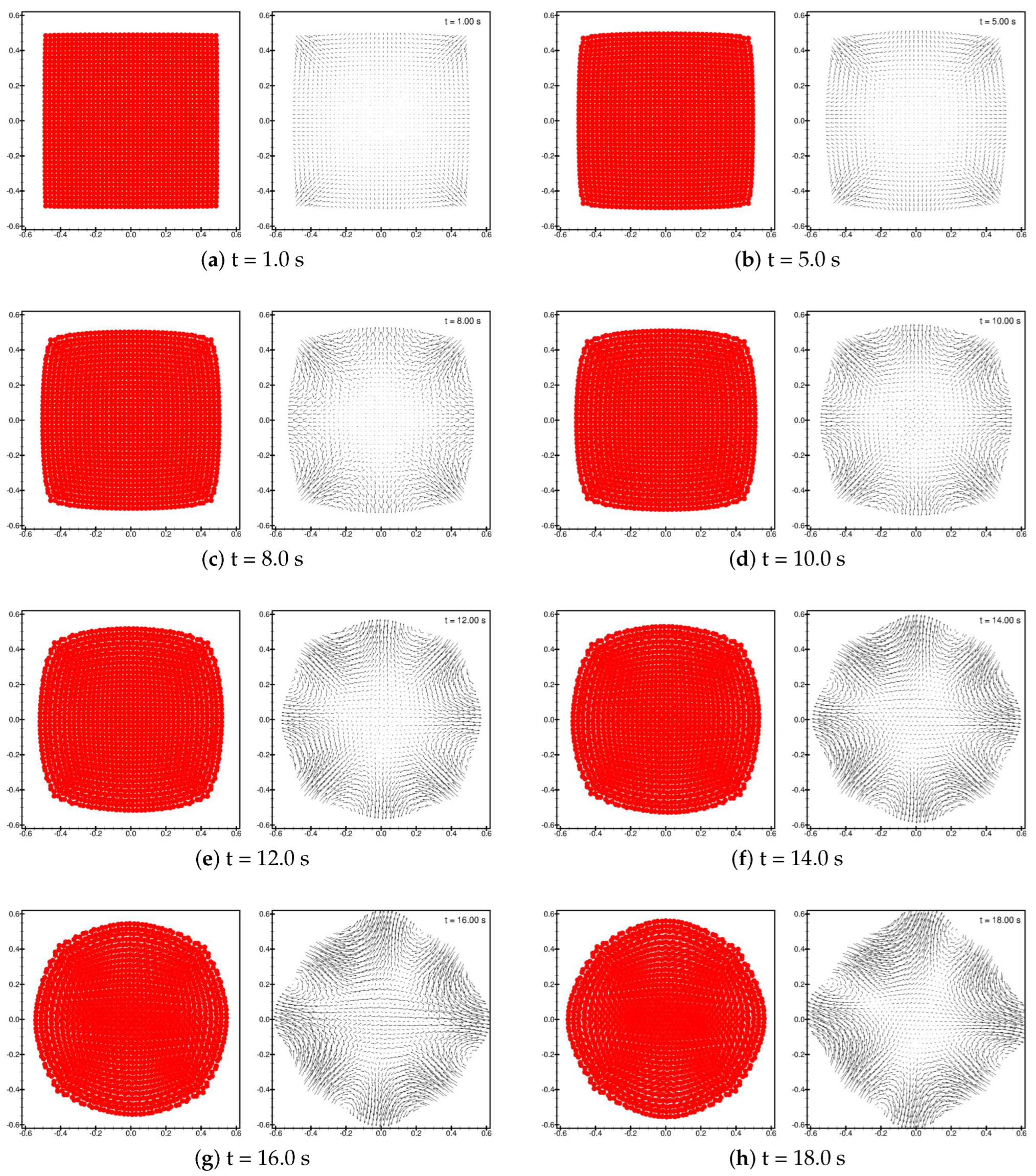
3.2. Validation Case 2 for the Surface Tension: A Square Drop with a Free Surface

This section shows a simulation of single-phase square drop by using the current surface tension force to show its capability for free surfaces. The parameters are listed in

Table 1. Parameters of used in the case of a square bubble in a single-phase system.

Parameters	Values
Width $W_B$ (m)	1.0
Number of particles $N_p$	1600
$\gamma$ in Equation (8) (-)	2
Reference pressure in EOS $p_r$ (Pa)	1.0
Background pressure in EOS $p_0$ (Pa)	1.0
Reference density in EOS ${\rho }_{ref}$ (kg/m${}^3$)	1.0
Viscosity of fluids ${\mu }_f$ (Pa·s)	0.001
coefficient of surface tension force $\sigma$ (N/m) (Pa·s)	10
Time step $\Delta t$ (s)	5.0 × ${10}^{-5}$
Time in simulation $T_t$ (s)	150.0

.

At the start, particles are arranged in a square array of zero velocity (Figure 3a). The surface tension forces are generated only at the four corners (Figure 3a). This clearly shows the validity and accuracy of the computed surface tension. Driven by the surface tension force, the fluid particles move gradually (Figure 3b–e). The particles at the corner move toward the center and the particles on the sides move outward. After 150 s (Figure 3e), the final distribution of particles becomes a nearly perfect disk.

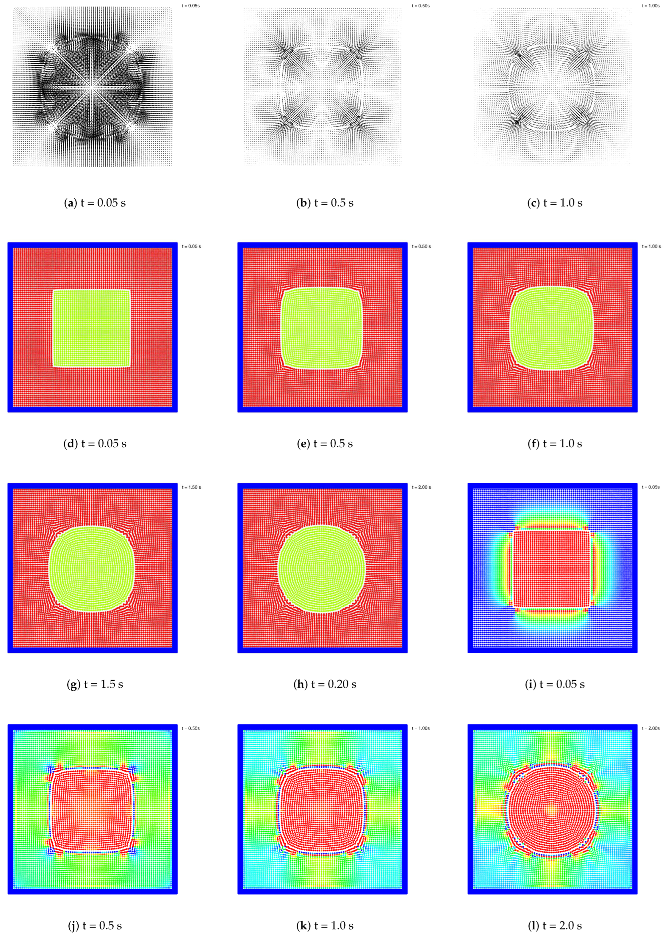
3.3. Validation Case 3 for the Surface Tension: A Square Bubble with an Inter-Phase Surface

Following a similar manner, the second case is a two-phase square bubble, whose evolution is shown in Figure 4. In this case, the coefficient of capillary force is enlarged about 7.2 times compared to the former case. The outside of the bubble is enclosed by fluids of higher density and lower viscosity (

Table 2. Parameters used in the case of a square bubble in a two-phase system.

Parameters	Phase ‘l’	Phase ‘g’
Width × height ($W_B\times H_B$) (m)	2.0 × 2.0	1.0 × 1.0
Number of particles $N_p$	4879	1521
$\gamma$ in EOS (-)	7	7
Reference pressure in EOS $p_r$ (kg/m${}^3$)	1.0	1.0
Background pressure in EOS $p_r$ (kg/m${}^3$)	1.0	1.5
Reference density in EOS ${\rho }_{ref}$ (kg/m${}^3$)	1.0	0.1
Viscosity of fluids ${\mu }_f$ (Pa·s)	1.0 × 10${}^{-3}$	1.0 × 10${}^{-6}$
coefficient of surface tension force $\sigma$ (N/m) (Pa·s)	72	72
Time step $\Delta t$ (s)	5.0 × 10${}^{-5}$	5.0 × 10${}^{-5}$
Time in simulation $T_t$ (s)	5.0	5.0

). Driven by the inter-phase surface tension force similarly, the central bubble has been changed from square to circular shape after about t = 2 s.

The velocity fields show the velocities particles in the four corners of the inner square move toward the center of it (Figure 4a–c). Figure 4d,f confirms the corresponding variations of particle positions of the bubble phase (shown by phase index of different colors). Moreover, at about t = 2.0 s, the inner square bubble becomes a nearly perfect circular bubble (Figure 4h). In addition, the pressure distributions at (t = 0.05, 0.5, 1.0 and 2.0 s) are shown in Figure 4i–l, respectively. The results of pressure distribution indicate the reliability of the current surface tension model. Hereafter, we would like to use the current model to simulate a typical case of a single rising bubble.

4. Numerical Results

4.1. Case A: A Single Rising Bubble

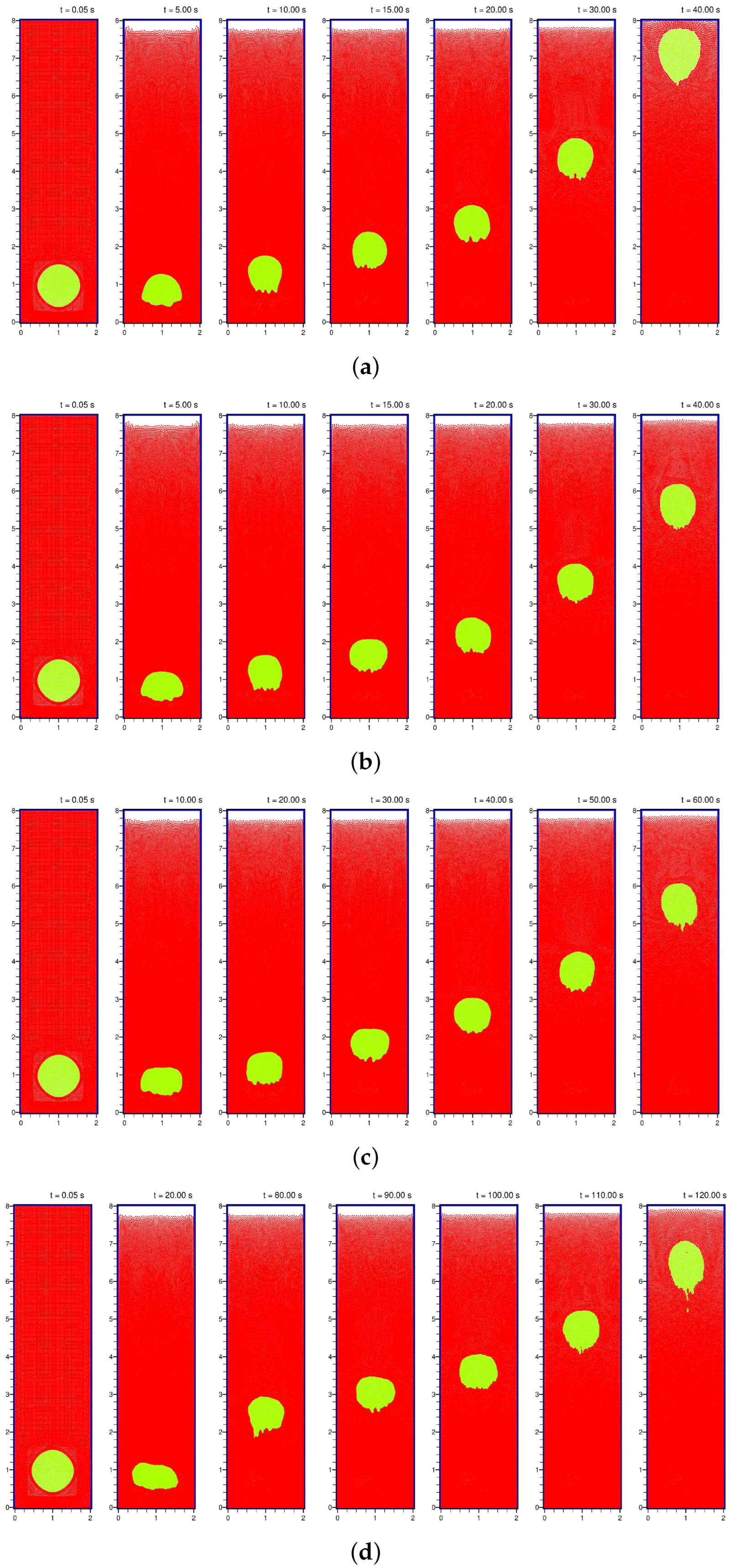
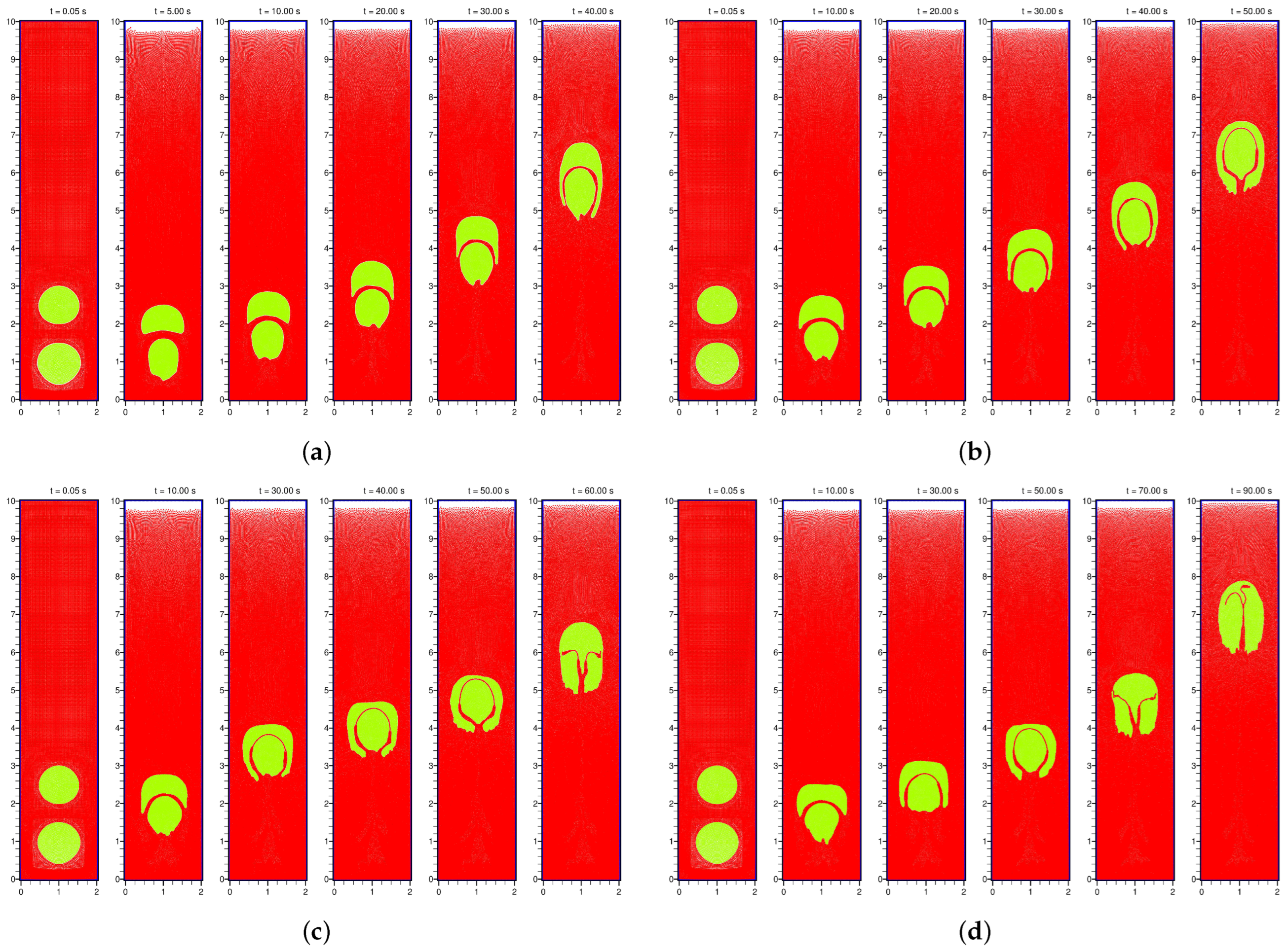
4.1.1. Snapshots of a Rising Bubble

As a demonstrative application of the current surface tension model, a rising single bubble in fluids is simulated here. Herein, a ’bubble’ does not mean it is a real bubble but just because its density is relatively smaller than the surrounding fluids. The density ratios are listed in

Table 3. Parameters used in Case A (CA) and Case B (CB) for rising bubbles in fluids.

Parameters	Phase ‘l’	Phase ‘g’
Width of Bed ($W_B$) (m)	2	-
Height of Bed ($H_B$) (m)	8 in CA & 10.0 in CB	-
Height of bubbles ($H_i$) (m)	-	1.0 and 2.5
Initial Diameter $D_i$ (m)	-	1
Number of particles $N_p$	24,273 in CA & 29346 in CB	1083 in CA & 2166 in CB
$\gamma$ in EOS (-)	7	7
Reference pressure in EOS $b_r$ (kg/m${}^3$)	1.0	1.0
Background pressure in EOS $p_r$ (kg/m${}^3$)	3.92	3.92
Reference density in EOS ${\rho }_{ref}$ (kg/m${}^3$)	1.0	-
Density ratios ($\frac{{\rho }_g}{{\rho }_f}$)	-	0.11, 0.22, 0.33, 0.44, 0.55
Viscosity of fluids ${\mu }_f$ (Pa·s)	2.0 × 10${}^{-4}$	2.0 × 10${}^{-4}$
Coefficient of surface tension $\sigma$ (N/m) (Pa·s)	0.72	0.72
Time step $\Delta t$ (s)	5.0 × ${10}^{-5}$	5.0 × ${10}^{-5}$
Time in simulation $T_t$ (s)	5.0	38∼125.0

, accompanied by other parameters. We use such a demonstrative case to show the capacity of the current model for simulating two-phase flows.

As shown in Figure 5a for $\frac{{\rho }_g}{{\rho }_f}=0.11$, a circular bubble of diameter 1 m is set in the bottom zone of a rectangular domain of size 2 m in width and 8 m in height (Table 3). At first, the bubble is compressed by surrounding fluid since it is immersed in it, with its volume soon becoming smaller and cap-like (Figure 5b). Then, as driven by the buoyant force of Equation (6), the bubble soon goes upward (Figure 5c–h). The velocity distribution around the rising bubble clearly shows the impact of the bubble’s motion on the surrounding fluid. When the bubble has risen close to the top, its volume also becomes larger.

Similarly, Figure 6 compares the rising process of the single bubble when the density ratio $\frac{{\rho }_g}{{\rho }_f}$ changes from 0.2 to 0.5. The bubbles in different cases go up ultimately. However, the speeds become slower and the bubble (in Figure 6d at $\frac{{\rho }_g}{{\rho }_f}=0.55$) almost needs more than three times of the time in (in Figure 6a at $\frac{{\rho }_g}{{\rho }_f}=0.22$) to get close to the top. During the rising process, the bubble’s shape is no longer maintained symmetrical and smooth. In particular, the shape profiles of the bubble’s tail always have been folded many times. The folded shape profiles in the downside of the rising bubble demonstrate the feature of the current surface tension force model, i.e., being capable of capturing the inter-phase interaction at particle scales.

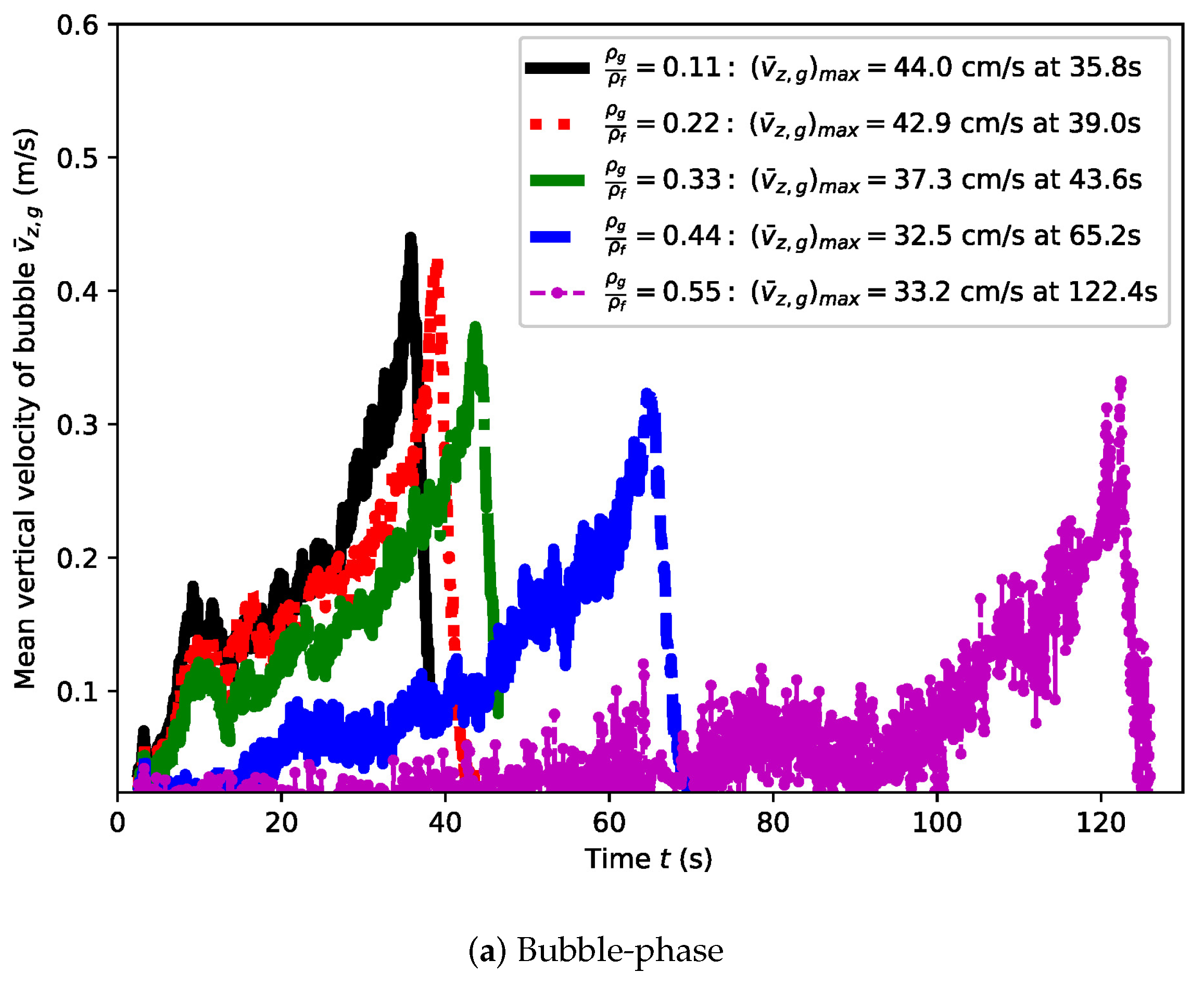
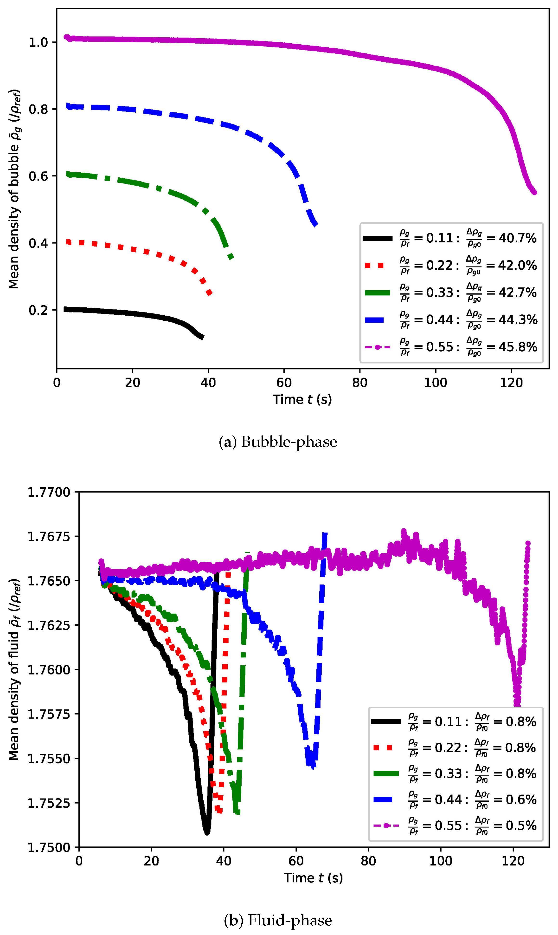
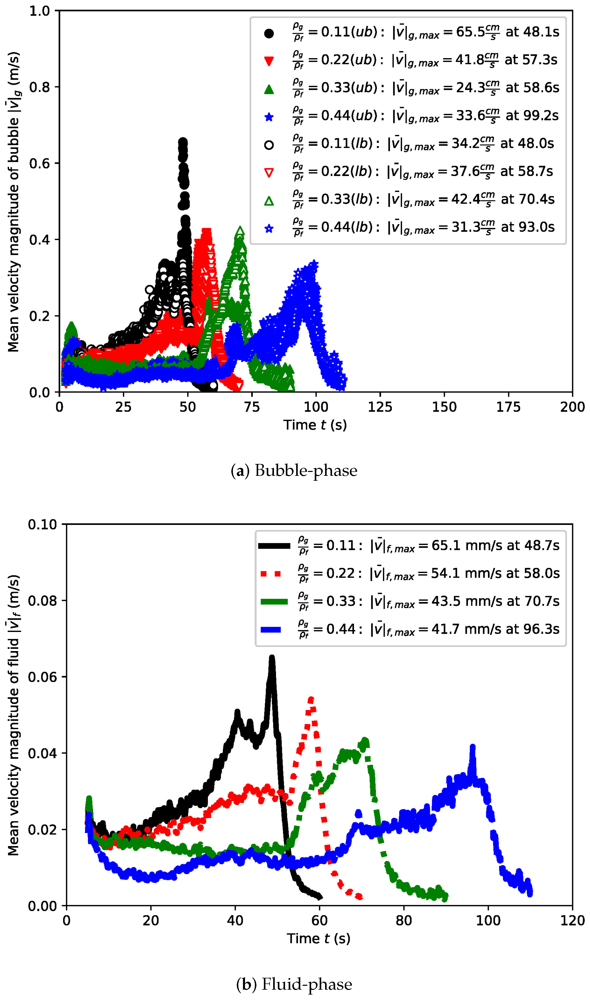
4.1.2. Rising Velocities and Densities

Then, the mean rising velocities of the bubble phase and surrounding fluids are computed, which are respectively defined as follows:

$$\begin{array}{c}\hfill \begin{array}{c}\hfill {\overline{V}}_{z,g}\left(t\right)=\frac{1}{V_g}\sum _{V_g}{V}_z\left(t\right)=\frac{1}{N_g}\sum _{i=1}^{N_g}{\left(V_z\right)}_i\left(t\right)\\ \hfill {\overline{V}}_{z,f}\left(t\right)=\frac{1}{V_f}\sum _{V_f}{V}_z\left(t\right)=\frac{1}{N_f}\sum _{j=1}^{N_f}{\left(V_z\right)}_j\left(t\right)\end{array}\end{array}$$

(17)

where the subscripts ‘g’ and ‘f’ denote the bubble and fluid phase, respectively. V is the volume and N is the number of particles belonging to each volume. z means the vertical direction (e.g., the z-direction).

Figure 7a,b shows the ${\overline{V}}_{z,g}\left(t\right)$ and ${\overline{V}}_{z,f}\left(t\right)$, respectively. For the bubble’s motion, ${\overline{V}}_{z,g}\left(t\right)$ is always going up from zero and quickly drops down after achieving its maximum at about t = 35–125 s in each case, respectively (Figure 7a). The maximum rising speed can be larger than 0.3 m/s. In addition, as the density ratio $\frac{{\rho }_g}{{\rho }_f}$ increases, the maximum rising speed of the bubble gently decreases, causing the time to achieve the maximum rising speed to be lengthened too (see the values in Figure 7a). This is reasonable since the buoyant force acting on the bubble should be weakened as the difference between the densities of the bubble and fluid becomes reduced. In contrast, for the fluids, although the rising velocities ${\overline{V}}_{z,f}\left(t\right)$ (Figure 7) are always negative (vertically downward), which are corresponding to the bubbles’ rising motion (vertically upward). Its magnitude is also always small (with a maximum magnitude lower than 0.03 m/s), about one order of magnitude smaller than that of the bubble’s rising velocity. The time points to achieve the peak velocities for both the bubble and fluid phase are almost simultaneous (see the time point values in Figure 7 corresponding to the maximum ${\left({\overline{V}}_{z,g}\right)}_{max}$ and ${\left({\overline{V}}_{z,f}\right)}_{max}$).

Similarly, the mean densities of the bubble and the surrounding fluid can be computed, respectively, by

$$\begin{array}{c}\hfill \begin{array}{c}\hfill {\overline{\rho }}_g\left(t\right)=\frac{1}{V_g}\sum _{V_g}{\rho }_g\left(t\right)=\frac{1}{N_g}\sum _{i=1}^{N_g}{\left({\rho }_g\right)}_i\left(t\right)\\ \hfill {\overline{\rho }}_f\left(t\right)=\frac{1}{V_f}\sum _{V_f}{\rho }_f\left(t\right)=\frac{1}{N_f}\sum _{j=1}^{N_f}{\left({\rho }_f\right)}_j\left(t\right)\end{array}\end{array}$$

(18)

As Figure 8 shows, the mean density of bubble ${\overline{\rho }}_g$ gently decreases as the bubble rises, and it can be reduced as much as more than 40% (see the values in the legend of Figure 8a). When the density ratio becomes larger, the amount of reduction of the density of the bubble becomes slightly larger (from 40.7% to 45.8%) too. The total amount of reduction of the bubble’s density is caused by the depressurization from surrounding fluids when the bubble goes from the height of z = 1 m to above 7 m. However, concerning the change of density of fluids, its relative magnitudes are always restricted within about 0.8% (Figure 8b), although the fluids may always become lighter when the bubble rises.

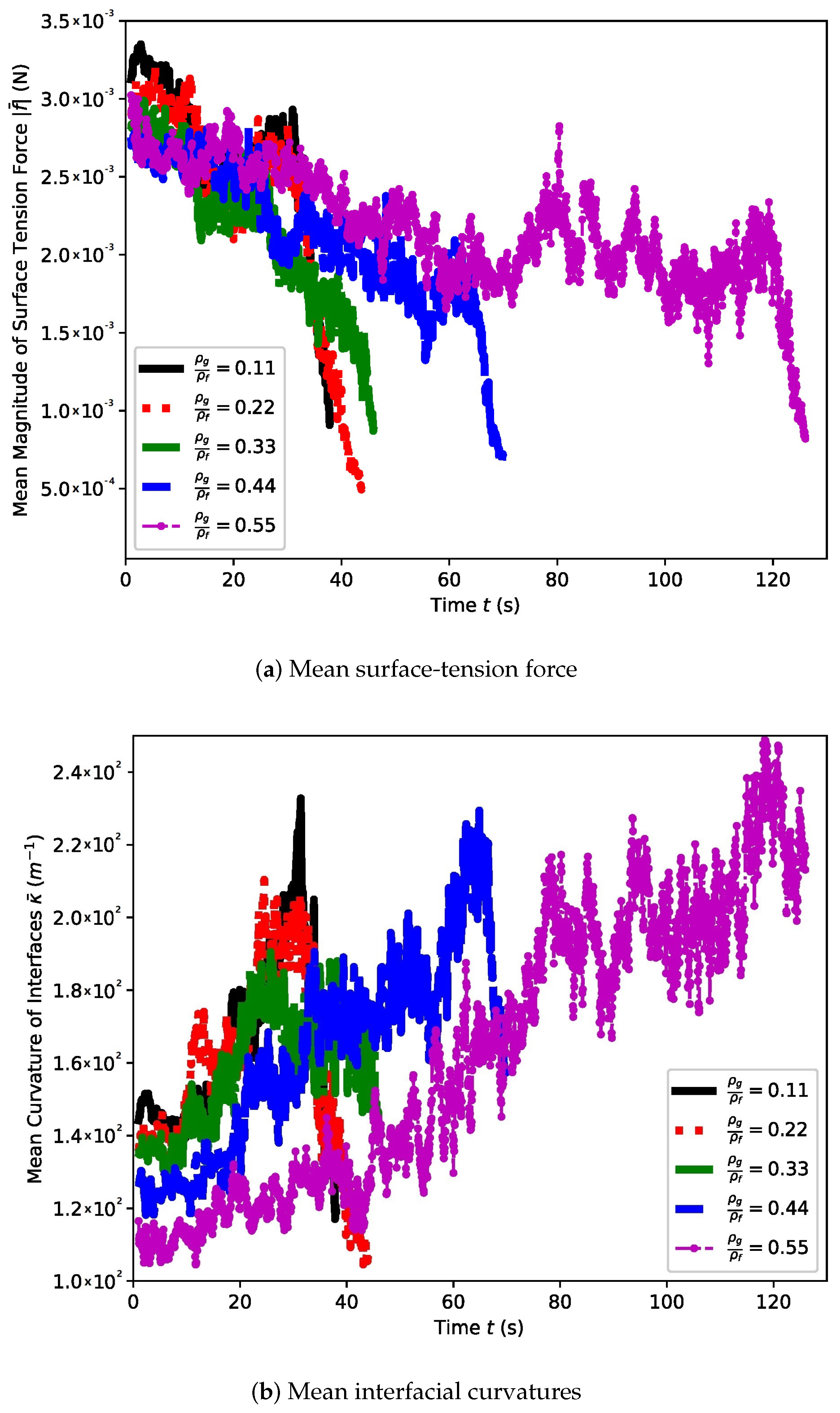
4.1.3. Mean Surface Tension Force, Curvature, and Its Power

In this section, the mean surface tension force, mean interfacial curvature, and mean power of the surface tension forces are computed as

$$\begin{array}{c}\hfill \begin{array}{c}\hfill {\overline{f}}_{Si}\left(t\right)=\frac{1}{N_g}\sum _{i=1}^{N_g}{f}_{Si}\left(t\right);{\overline{\kappa }}_f\left(t\right)=\frac{1}{N_g}\sum _{j=1}^{N_g}{\kappa }_j\left(t\right);{\overline{P}}_f\left(t\right)=\frac{1}{N_g}\sum _{j=1}^{N_g}{f}_{Si}\left(t\right)·v_i\left(t\right)\end{array}\end{array}$$

(19)

Herein, we will use them to explain the features of the current particle-scale surface tension force model.

As Figure 9 shows, the mean surface tension force is generally decreasing as the bubble rises. This is reasonable because (1) the surface tension force is caused by the imbalance between the interactions of molecules on the two sides of the interfacial surface. (2) When the bubble rises, the materials of either bubble or fluid are kept the same. However, the densities of either the bubble or fluids are changed (as indicated by Figure 8). The varied densities cause the density difference between the fluids and the bubble reduction as the bubble rises. (3) The reduced density difference makes the imbalance of interactions on the two sides of the interface weakened. In particular, in the current simulation, the number densities of the bubble-phase particles and the fluid-phase particles will change which explains the weakened interactions on the two sides of the interface.

In Figure 9b, it is also noticed that the interfacial curvature of the current model is also increasing as the bubble rises. This means that the overall level of interfacial curvature is not mainly determined by the time how long the bubble is evolved. Instead, it is mainly determined by where the bubble is located. As the number of bubble particles is kept the same when the bubble moves, the location of the bubble (namely, the height where the bubble is located) may determine the level of the number density surrounding the bubble, i.e., determines the number of interfacial interaction pairs. When the bubble rises, the bubble’s volume becomes large. More interfacial interaction pairs may take place, and the interfacial geometric feature may become more and more un-smoothing (non-round) at particle-scale (see Figure 5 and Figure 6). That is why the particle-scale curvature is increasing as the bubble rises.

Notice that the smoothing length is proportional herein to $\sim {\left(\frac{m}{\rho }\right)}^D$. As the mass of the particle is kept the same, the variation of density may change both the smoothing length as well as the volume of the particle. In other words, $\overline{h}$ is an indicator of the variation of the volume of the particle. Figure 10a shows variations of the smoothing length $\overline{h}$ of the bubbles in both cases. It is shown that the $\overline{h}$ is increasing when the bubbles rise, namely when the density becomes smaller. This confirms the explanations mentioned in the former paragraph on the bubble’s volume variation. In addition, $\overline{h}$ becomes larger when the $\frac{{\rho }_g}{{\rho }_f}$ is larger, which is straightforward since the mass of the particle of the bubble is larger when $\frac{{\rho }_g}{{\rho }_f}$ is larger.

Additionally, the power of surface tension force (Figure 10b) is determined by both the vector of surface tension force $f_{Si}$ and the velocity $v_i$. As discussed above, the surface tension force becomes weakened (Figure 9b) and the rising speed (Figure 7a) is reduced as the density ratio $\frac{{\rho }_g}{{\rho }_f}$ increases. Therefore, the surface tension force becomes lower as the density ratio $\frac{{\rho }_g}{{\rho }_f}$ increases.

4.2. Case B: A Pair of Rising Bubbles

To further demonstrate the capability of the current model, this section shows the simulation of a pair of initially vertically arranged but separated bubbles. Given $\frac{{\rho }_g}{{\rho }_f}=0.11$∼0.44, Figure 11 shows the snapshots of the evolution of the pair of rising bubbles. The two bubbles merge into a larger one when they rise. Although given a round initial shape for the two bubbles, the lower bubble (designated as ‘lb’) forms a slender shape whereas the upper bubble (named ‘ub’ for short) forms a cap-like shape. The ‘lb’ seems to have a larger rising velocity than the ‘ub’, which causes the ‘lb’ to collide into the ‘ub’ and become a kernel of the ‘ub’ (Figure 11b,c), or a head bubble dragging the ’ub’ (Figure 11c).

Figure 12a,b shows similar processes of change of densities as the former case. Compared to Case A, the amount of density reduction of the gas-phase becomes smaller (with only about 37–38%). However, the changes of densities of both the ‘lb’ and ‘ub’ are almost coinciding. In addition, the duration for the two bubbles to reduce the density becomes longer than in Case A. Similar trends can also be seen in Figure 12b. The fluids’ variation in density also becomes slower than in Case A, although its relative changes can normally be omitted.

Although the variations of densities of the two bubbles can be hard to distinguish from each other, the differences in rising velocities of the two bubbles have clear discrepancies (Figure 13a). When the density ratio is low ($\frac{{\rho }_g}{{\rho }_f}=0.11$), the maximum rising velocities of the two bubbles are 65.5 cm/s and 34.2 cm/s, respectively (about two times of magnitudes). In contrast, when the density ratio is large ($\frac{{\rho }_g}{{\rho }_f}=0.55$), the maximum rising velocities of the two bubbles are almost the same (33.6 cm/s and 31.3 cm/s, respectively). This trend shows the clear feature when the density ratio is large, the bubbles’ motion velocities may be different even if they stay close to each other. Additionally, the fluid’s maximum velocity may also become smaller when the density ratio $\frac{{\rho }_g}{{\rho }_f}$ increases.

Finally, Figure 14 shows the variations of smoothing length for each bubble (${\overline{h}}_g$ for the ‘lb’ and ‘ub’, respectively) and fluid (${\overline{h}}_f$) in the two-bubble case. It is shown that ${\overline{h}}_f$ is almost independent of $\frac{{\rho }_g}{{\rho }_f}$ and time. However, ${\overline{h}}_g$ is always increasing as either the bubbles rise or the $\frac{{\rho }_g}{{\rho }_f}$ increases. As explained before, the rise of the bubble may cause depressurization and expansion of the bubbles. As a consequence, this makes ${\overline{h}}_g$ larger dynamically determined by the location of the bubbles. Therefore, as the two bubbles merge into a large one, the locations of the materials belonging to the two bubbles are almost at the same level of heights. Hence, ${\overline{h}}_g$ of either the ‘lb’ or ‘ub’ is almost overlapping. In addition, the change of ${\overline{h}}_g$ by varied $\frac{{\rho }_g}{{\rho }_f}$ is caused by the large mass given initially, which is determined by the static condition given for each case.

5. Further Discussion

In this work, one can observe that the bubble interfaces are not as smooth as those commonly seen in simulations through Eulerian methods. The reasons are explained as follows: the surface tension is solved based on the geometrical configuration of every particle to every neighboring particle, at least one of which is located within the thin region of ‘fluid’–‘gas’ interfaces. The smoothing particle hydrodynamics is based on the technique of locally smoothing to gain a macroscopic quantity, such as density, velocity, etc. Therefore, when computing the surface tension force based on every pair of particles located within the interface, it means the scale of computing the surface tension force is thin enough in the order of or even thinner than interfaces. This condition is just like modeling and observing the surface tension via a microscope. That is why the interface surface is not as smooth as that always seen in existing works.

In addition, although the surface tension force is computed from such a fine scale, a large coefficient of surface tension was still used which is equivalent to its empirical or macroscopic counterpart through locally smoothing techniques. Therefore, the surface tension force is strengthened compared to a practical case. Therefore, bubble convergence does not happen as easily as usually seen. In other works, the bubbles do not have a kinetic energy large enough to break up the surface tension on the interface to form a convergence. This case is always seen in fine-scale bubbles. However, the current results indicate that it may also take place for large bubbles providing the surface tension is large enough.

Note that every particle in the SPH can be viewed to represent a number of small molecules, whose scale is far larger than each molecule of fluids to guarantee meaningful means of fluid quantities, and far smaller than the macroscopic flow scale to justify the derivatives of fluid quantities in the Navier–Stokes equation. In most existing CSF and CSS methods, a smoothing operation is always needed before computing the gradient of the geometry of interfaces to obtain the STF. Different from these existing models, the definition of the gradient of the geometry of interfaces for obtaining the STF here is ahead of the smoothing operation. In other words, the method proposed here is based on the computations of STF caused by every pair of neighboring particles on the interface before the smoothing operation, where the pair of particles belong to different phases. To some extent, this method can be viewed as a mesoscale method to get the STF. After computing the STFs at the mesoscale, the STFs are imposed on each neighboring particle through the smoothing operation. Therefore, the result presented in this work would not be as smooth and symmetrical as presented in most existing continuum-based methods (not only by the CSF or CSS method but also by the VOF or front-tracking method). However, this method would be beneficial to further implementing additional mesoscale modeling of interfacial mechanisms.

Moreover, the mesoscopic modeling of surface tension force is through every pair of particles on the interface. Given the STF force coefficient is large enough, the bubbles sometimes cannot break up the surface tension force to merge (Figure 11). The coefficient of STF is practically based on the macroscopic scale in reality, whereas it is used on the mesoscopic scale here. This means that the STF here is too strong to break up by the motion of the bubble. Therefore, the bubble sometimes cannot merge during the rising process until it impinges on the top wall. We would like to explain this issue here, as we still do not know what value should be given to the mesoscopic coefficient of STF.

6. Conclusions

Based on the interfacial geometric shape and the gradient of the densities across the interface, the particle-scale surface tension force model proposed herein has been proven to be suitable for capturing the interfacial interactions. The STF model is not always in the direction according to perfect interface geometry. Instead, it depends on specific particle locations near the interface. In particular, the thickness of the interface is dependent on the smoothing length which is related to the density of the bubble of fluids. Therefore, either one layer or two-layer thickness of the interface may be incorporated into the current model.

The dam-break case is utilized to validate the current combined kernel and the application of the STF model in simulating the evolution of a square bubble of a single-phase system or a square bubble immersed in the other fluids provides a suitable validation for the current model. After validations, the characteristics of the rising bubbles are studied by using the current STF model. Based on the simulation results, the bubble’s rising velocities are almost one order of magnitude larger than the fluids. The densities of bubbles are reduced by about 40% from the deeply immersed bottom to the top of fluids, whereas the densities of fluids change only about 1%. The STF is decreasing and the curvature is increasing during the bubbles’ rise. This is mainly caused by the decrease in densities between the bubbles and fluids when the bubbles rise since the bubbles in lower heights have large densities, whereas they have lower densities after rising higher. The smoothing length’s variation confirms the change of bubbles’ expanded volume and reduced density. Therefore, larger differences between the bubble and the immersed fluids indicate larger surface tension force, larger maximum velocity, shorter time duration, and larger power of STF, and vice versa.

The rising of a pair of bubbles shows a little bit less variation in densities of bubbles than in the single bubble case. In addition, larger differences in bubbles’ and fluids’ densities result in large differences in the peak velocities between the two bubbles, although the bubbles stay close and merge into a single one during their rising processes. The densities and smoothing lengths of the two bubbles seem to be almost the same since they always merge into a large one. Additionally, the variation of fluids is almost independent of the ratios of densities of bubbles to fluids.

References

1. Mittal, H.; Ray, R.K.; Gadêlha, H.; Patil, D.V. A coupled immersed interface and level set method for simulation of interfacial flows steered by surface tension. Exp. Computat. Multiphase Flow 2021, 3, 21–37. [Google Scholar] [CrossRef]
2. Liu, J.M.; Wang, Y.Q.; Gao, Y.S.; Liu, C. Galilean invariance of Omega vortex identification method. J. Hydrodyn. 2019, 31, 249–255. [Google Scholar] [CrossRef]
3. Lin, M.; Zhong, M.; Li, Y.; Yuan, M.; Yang, Y. Numerical analysis on molten droplet hydrodynamic deformation and surface waves under high pressure pulse. Ann. Nucl. Energy 2015, 77, 133–141. [Google Scholar] [CrossRef]
4. Osher, S.; Fedkiw, R.P. Level Set Methods: An Overview and Some Recent Results. J. Comput. Phys. 2001, 169, 463–502. [Google Scholar] [CrossRef]
5. Tryggvason, G.; Bunner, B.; Esmaeeli, A.; Juric, D.; Jan, Y.J. A Front-Tracking Method for the Computations of Multiphase Flow. J. Comput. Phys. 2001, 169, 708–759. [Google Scholar] [CrossRef]
6. Liu, C.; Xu, H.; Cai, X.; Gao, Y. Chapter 6—Liutex and third generation of vortex identification methods. In Liutex and Its Applications in Turbulence Research; Liu, C., Xu, H., Cai, X., Gao, Y., Eds.; Academic Press: Cambridge, MA, USA, 2021; pp. 119–149. [Google Scholar]
7. Krimi, A.; Rezoug, M.; Khelladi, S.; Nogueira, X.; Deligant, M.; Ramírez, L. Smoothed Particle Hydrodynamics: A consistent model for interfacial multiphase fluid flow simulations. J. Comput. Phys. 2018, 358, 53–87. [Google Scholar] [CrossRef]
8. Zhu, Y.; Qiu, Z.; Xiong, J.; Yang, Y. Verification and validation of MPS potential force interface tension model for stratification simulation. Ann. Nucl. Energy 2020, 148, 107753. [Google Scholar] [CrossRef]
9. Hoogerbrugge, P.J.; Koelman, J. Simulating Microscopic Hydrodynamic Phenomena with Dissipative Particle Dynamics. EPL (Europhys. Lett.) 1992, 19, 155–160. [Google Scholar] [CrossRef]
10. Abdolahzadeh, M.; Tayebi, A.; Omidvar, P. Thermal effects on two-phase flow in 2D mixers using SPH. Int. Commun. Heat Mass Transf. 2021, 120, 105055. [Google Scholar] [CrossRef]
11. Wang, Z.B.; Rong, C.; Hong, W.; Liao, Q.; Zhu, X.; Li, S.Z. An overview of smoothed particle hydrodynamics for simulating multiphase flow. Appl. Math. Model. 2016, 40, 9625–9655. [Google Scholar] [CrossRef]
12. Vergnaud, A.; Oger, G.; Touzé, D.L.; DeLeffe, M.; Chiron, L. C-CSF: Accurate, robust and efficient surface tension and contact angle models for single-phase flows using SPH. Comput. Methods Appl. Mech. Eng. 2022, 389, 114292. [Google Scholar] [CrossRef]
13. Brackbill, J.U.; Kothe, D.B.; Zemach, C. A continuum method for modeling surface tension. J. Comput. Phys. 1992, 100, 335–354. [Google Scholar] [CrossRef]
14. Lafaurie, B.; Nardone, C.; Scardovelli, R.; Zaleski, S.; Zanetti, G. Modelling merging and fragmentation in multiphase flows with SURFER. J. Comput. Phys. 1994, 113, 134–147. [Google Scholar] [CrossRef]
15. Amt, A.; Ap, B. Pairwise Force Smoothed Particle Hydrodynamics model for multiphase flow: Surface tension and contact line dynamics. J. Comput. Phys. 2016, 305, 1119–1146. [Google Scholar]
16. Scardovelli, R. Direct Numerical Simulation of Free-Surface and Interfacial Flow. Annu. Rev. Fluid Mech. 2003, 31, 567–603. [Google Scholar] [CrossRef]
17. Nugent, S.; Posch, H.A. Liquid drops and surface tension with smoothed particle applied mechanics. Phys. Rev. E 2000, 62, 4968–4975. [Google Scholar] [CrossRef]
18. Zhang, M.Y.; Zhang, H.; Zheng, L.L. Simulation of droplet spreading, splashing and solidification using smoothed particle hydrodynamics method. Int. J. Heat Mass Transf. 2008, 51, 3410–3419. [Google Scholar] [CrossRef]
19. Crespo, A.; Gomez-Gesteira, M.; Dalrymple, R.A. Modeling Dam Break Behavior over a Wet Bed by a SPH Technique. J. Waterw. Port Coast. Ocean Eng. 2008, 134, 313–320. [Google Scholar] [CrossRef]
20. Farzin, A.S.; Fatehi, B.R.; Hassanzadeh, C.Y. Position explicit and iterative implicit consistent incompressible SPH methods for free surface flow. Comput. Fluids 2019, 179, 52–66. [Google Scholar] [CrossRef]
21. Ye, Y.; Xu, T.; Zhu, D.Z. Numerical analysis of dam-break waves propagating over dry and wet beds by the mesh-free method. Ocean Eng. 2020, 217, 107969. [Google Scholar] [CrossRef]
22. Jánosi, I.; Jan, D.; Szabó, K.; Tél, T. Turbulent drag reduction in dam-break flows. Exp. Fluids 2004, 37, 219–229. [Google Scholar] [CrossRef] [Green Version]
Figure 1. Sketch of particle-scale surface tension force on the interface of the internal bubble and the surrounding fluid.
Energies 15 07132 g001
Figure 2. Comparison of dam-break process using the current kernel with some numerical [19,20,21] and experimental [22] results. (a) t = 0.280 s; (b) t = 0.345 s; (c) t = 0.470 s.
Energies 15 07132 g002
Figure 3. The evolution of particle position and velocity for a single-phase square bubble. The coordinate axes are x in horizontal and y in vertical directions, and the same hereafter if not specified.
Energies 15 07132 g003
Figure 4. The evolutions of velocity (ac), phase index (dh), and pressure (il) of particles in the two-phase square bubble.
Energies 15 07132 g004
Figure 5. The evolution of one rising bubble (ah) and corresponding velocity fields (ip) with density ratio ρ g ρ f = 0.11 .
Energies 15 07132 g005
Figure 6. The evolution of one rising bubble with density ratio ρ g ρ f = 0.22 (a), 0.33 (b), 0.44 (c), and 0.55 (d), respectively.
Energies 15 07132 g006
Figure 7. The mean vertical velocities V ¯ z of the bubble (a) and the surrounding fluid (b) for different density ratios ρ g ρ f = 0.11–0.55.
Energies 15 07132 g007aEnergies 15 07132 g007b
Figure 8. The mean densities ρ ¯ of the bubble (a) and the surrounding fluids (b) for different density ratios ρ g ρ f = 0.11–0.55.
Energies 15 07132 g008
Figure 9. The mean force | f | ¯ (a) and mean curvature κ ¯ f (b) of the surface tension force for different density ratios ρ g ρ f = 0.11–0.55.
Energies 15 07132 g009
Figure 10. The mean smoothing length h ¯ (a) and the mean power P ¯ f (b) of the bubble case for different density ratios.
Energies 15 07132 g010
Figure 11. The evolution of a pair of rising bubbles with density ratio ρ g ρ f = 0.11 (a), 0.22 (b), 0.33 (c), and 0.44 (d), respectively.
Energies 15 07132 g011
Figure 12. The mean densities ρ ¯ g of the bubble (a) and the surrounding fluids (b) for different density ratios ρ g ρ f = 0.11–0.44.
Energies 15 07132 g012
Figure 13. The mean magnitudes of velocities of the bubble | v | ¯ g (a) and the surrounding fluids | v | ¯ f (b) for different density ratios ρ g ρ f = 0.11–0.44.
Energies 15 07132 g013
Figure 14. The mean smoothing length h ¯ of the two-bubble case for different density ratios.
Energies 15 07132 g014