Abstract
South Korea officially committed to reducing 40% of its total carbon emissions by 2030, but the country has a carbon-dependent economic structure based on the manufacturing industry. Additionally, the industrial structure of each region in South Korea is heterogeneous. In this regard, policymakers should analyze the carbon emission condition at a regional level because abatement aspects are heterogeneous by urban spatial production. However, although various studies have developed a methodology to evaluate the GHG emission condition, these studies failed to consider the fundamental aspect of regional heterogeneity. In this regard, this study suggests a quantitative method to assess the potential of the carbon neutrality of regions and industries by using both shift-share analysis and the Log Mean Divisia Index method. Shift share analysis is used to quantify the relation between the industry and regional characteristics, and the Log Mean Divisia Index method can decompose each effect for economic growth and technological progress. By combining these two methods, this study suggests four classifications to evaluate regional and industrial characteristics of GHG emissions and analyze each region’s emission status in terms of the mining and manufacturing industry in South Korea.
1. Introduction
South Korea officially committed to reducing 40% of the total national GHG emissions by 2030, compared with the value in 2018. However, Korea has a carbon-dependent economic structure in that the industry sector occupies a vast proportion of the national economy. In particular, since Korea has a manufacturing-based economic system with high emissions, it is difficult for a national government to reduce total emissions compared to other countries. Nevertheless, as achieving carbon neutrality becomes a political priority, the government is actively looking for methods and ways to achieve both economic growth and emission reduction simultaneously. Additionally, in Korea, the industrial structure of each region is heterogeneous. These regional and industrial characteristics make it challenging to manage carbon emissions at the national level.
As part of this concern, various policy methods are now being discussed, but these methods have not yet yielded sufficient results to achieve NDC (Nationally Determined Contributions) goals. To achieve a social consensus and challenging goals on carbon neutrality, an appropriate methodology is needed for each industrial sector to evaluate its emission performance. Such an approach ensures the fair mean equality of opportunities and reasonable compensation for performances. In this regard, this study suggests an integrated performance measurement methodology to evaluate heterogeneous geographical GHG emission activities. To establish an integrated measurement method to evaluate local and regional GHG emission activities, this study uses both Logarithmic Mean Divisia Index (LMDI) and shift-share analysis. By examining the current GHG emission status in the industry and regional sectors through this methodology, this study tries to confirm whether it is realistically possible to achieve both economic growth and emission reduction simultaneously. Additionally, this study aims to give information regarding the current condition of carbon abatement performance by regions which can help national and local policymakers to modify emission goals and related plans more realistically. Furthermore, if the exact condition of GHG abatement performance is provided, it will help each local government to build comprehensive emission management. Additionally, through performance monitoring, local economic agents could be motivated by previous performance evaluations. In more detail, this study aims to explore the following two research questions.
- This study aims to check whether urban economic structure interrelates with GHG emissions through quantitative empirical analysis.
- This study tries to check how heterogeneous industrial structure by region affects local carbon emission by assessing it through the integrated performance evaluation method.
2. Literature Review and Theoretical Prospect
Over the last few decades, the relationship between carbon emissions and cities has received increasing attention from various academic fields. In early studies, the differences in climate conditions between urban regions and rural regions are mainly discussed. These studies particularly focused on the urban heat island effect caused by urban structure and warned that policy decision-makers should consider climate change mitigation strategies in urban planning [1,2,3,4,5,6,7]. Even though these early studies broaden urban planning to consider climate, they are limited to dealing with complex climate issues only at the local level [8,9]. In recent years, many studies have tried to look at the urban climate issue from a comprehensive and comparative perspective. Still, a globally agreed-upon protocol to deal with urban climate issues has not been established sufficiently [10].
Studies on low-carbon urban economy growth commonly approach carbon neutrality with urban planning. One study, which covers the concept of urban carbon transformations, suggests that local GHG emission blocks are divided by geographical and economical industrial territories. Some other studies imply that urban networks have a significant influence on global carbon emissions [11,12,13]. As such, policymakers dealing with urban carbon emission issues should consider local geographical and industrial contexts and international networks surrounding the city. Global agreements and protocols on climate change have a consistent influence on urban policy-making [14]. Global city governments are forced to incorporate carbon neutrality strategies into local urban policy and urban planning strategies [15]. Korea, whose GHG emissions occupy a large pie of global climate change, also has been trying to integrate carbon neutrality into urban planning. In this context, Korea set goals to incorporate urban issues into the national carbon neutrality strategy for 2050 [16,17,18].
Urban structure, including physical, social, geographical, and economic characteristics, influences carbon emission. Some studies on urban systems imply that physical urban land use derived from government policies affects future GHG emissions [19]. Together with urban structure, human activities also significantly impact local GHG emissions [20,21]. These results imply that well-designed urban policy and urban planning can influence and manage its GHG emission level. A series of studies commonly point out that urbanization directly reduces GHG emissions per person [22]. Furthermore, the city-level analysis of GHG inventory in China shows GHG uncertainty caused by industrial structure, economic growth, and population. These studies prove that the urban regional GHG emission level is destined for complex variables, meaning equity and allocation are not easily defined [23]. Government policy at the regional city level also contributes to GHG emission change. In the case of Spain, each province conducts different tax-related policies to manage GHG. Spatial clustering results are in strong interaction with one another [24,25]. Of course, GHG emission aspects are not perfectly dependent on regional territories. International companies are vague when pertaining to the places where they emit GHG exactly. Nevertheless, the spatial performance of each GHG abatement can be sorted geographically because the dynamics ultimately depend on each area [26]. Many studies that analyzed the Korean industry have already suggested the regional level of GHG emission value. Not only is the measurement needed to judge whether the GHG abatement objective is approachable, but the evaluation also motivates agents to move toward the goal voluntarily [27].
The Shift-share analysis is one of the traditional methodologies to quantify the relation between industry structure and regional characteristics. It is a quick and inexpensive analysis tool for scattered and decentralized data. If sound statistical basis sets are used for shift-share analysis [28], they can be applied to the study of regional structure. As such, this study chooses the classification of 17 urban regions. Some studies indicate that estimating the inefficiency and checking its drivers for policymakers is essential. It seems applicable to the part of GHG emission [29]. Other studies with theoretical bases support the opinions regarding the importance of efficiency evaluation [30]. One study, for example, uses stochastic frontier analysis when evaluating GHG efficiency. In particular, a Chinese study has analyzed the relationship between industrial structure and the nation’s efficiency. It concluded that the systems of energy use significantly impact GHG emissions, turning in indirect evidence [31]. Suggested flows of theoretical framework focus on what characteristics of each sort and how much they influence the GHG emission quantity of each agent behavior. In other words, evaluation needs to set the target with a standard unit of carbon or energy consumption, the kind of behavior, and so on [32]. Such a target is mainly represented by the concept of carbon intensity (CI). This concept is an effective tool for the emission agent behavior, which means the ratio between the units of the GHG emission and the output of productivity. Many studies investigated carbon emission use CI in a proper value evaluation of the performance of abatement potential [33,34,35,36].
Furthermore, to extract valuable data for analysis, only the carbon emission quantity per good measured by value added is not enough to conduct research. What factor is chosen and how much the factor influences the intensity should be sorted. Various methodologies have been put forward for several decades. Studies suggest classifying what factors influence energy consumption with a revised method. A study decomposes the energy intensity ratio into some elements and suggests which factor functions to spend energy during production [37]. In the late decade, the methodology has been standardized into a specific form. Slight variations are applied; however, the macroscopic perspective of methodology is generalized. The following studies are representative examples. One study decomposes factor CO2 emissions into a population, GDP per capita, and carbon intensity of production [38]. Many studies analyzing Korea’s status also suggest various models by focusing on industrial structure. They found out that the technology level of industries can influence the effort of GHG abatement. This implies the existence of heterogeneity in intra-sector emission abatement potential [39].
Log Mean Divisia Index (LMDI) is also applied internationally. The index derived by decomposition analysis compares Pakistan, India, and China, and it shows decoupling due to environmental impact from economic growth [40]. In addition, the studies indicate that LMDI is an effective way to conduct decomposition analysis in evaluating carbon emission and the potential of abatement performance [41,42]. Details of LMDI methodologies are analyzed next by selecting an affordable form.
3. Methodology and Data
3.1. Methodology—Logarithmic Mean Divisia Index (LMDI) and Shift-Share Analysis
To evaluate national performance sorted by each industrial sector, this study uses LMDI and shift-share methods. LMDI is an ideal index for interpreting composed data and adding essential variables to measure economic change. The critical visible factor of fundamental economic instability, such as GHG emission, infers that the GHG emission can be decomposed from other related factors. Additionally, statistical residuals do not occur in the LMDI analysis result, which helps researchers to achieve effective outcomes [43]. In this regard, many studies have analyzed the factors contributing to GHG emissions during the last decade, i.e., [44,45].
Recently, many researchers have analyzed the GHG emissions of industrial sectors using LMDI, especially in China and Korea [46,47]. Notably, one research study that examined the Korean industry of 2017 pointed out that Korea is shifting from an energy-intensive business to high-tech manufacturing. This change implies that government should reduce energy consumption while maintaining economic growth [48], and also implies that policies regarding GHG emissions should concern both economic growth and technical GHG intensity. The national economic condition affects the growth of every industrial sector. Additionally, the growth of national industry influences the growth of local and regional industries-. In this respect, Shift share analysis can help extract regional-specific characteristics. The one advantage of shift-share analysis is that it excludes the external factors affecting the industrial sector. Lately, shift-share analysis mainly depends on employment change in the industrial structure [49]. Furthermore, shift-share analysis has been actively applied to analyze the energy consumption of provinces, which often visualize its results [50].
In the preceding research, both LMDI and shift-share analysis are used to analyze GHG emissions through the employment unit. The economic growth effect and GHG intensity effect measured by GHG emission change with LMDI can be extracted through shift-share growth, resulting in GHG emission quantities as change effects.
3.2. Data
This study set the time range of the data from 2016 to 2019. This is because of the data availability. The Korean government has built up GHG emission performance statistics with CO2 equivalent ton unit from 2016. The 2019 data sets are the latest due to the COVID-19 pandemic. The pandemic also has the possibility to distort long-term GHG emission performance by undervaluing GHG risks. For this reason, the period from 2016 to 2019 was selected for this study.
The scope of the industrial sector is the MM industry in Korea, which contributes to most of the GHG emission inventory. As the energy supply is a significant consumption of GHG inventory, the concept for the ratio of the GHG consumption of the MM industry to the total GHG consumption of all sectors also reflects the contribution. According to GHG inventory statistics of Statistics Korea (KOSTAT), 56% of the total GHG industry consumption of GHG and 65% of the total GHG industry consumption were used in the mining manufacturing sector in 2018. The references of data used are as follows.
- (1)
- Korea Energy Agency arranged the energy and GHG emission inventory data. Industrial Sectors Energy and GHG Emission Statistics in 2017 and the same document in 2020 provided Industrial Sectors Energy and GHG Emission Statistics from Korea Energy Agency from 2017 to 2020.
- (2)
- Korea Bank provided data, gross output, and value-added of each company sorted by sectors, with 2015 as the reference year. Korean Standard Industrial Classification, Classification of Individual Consumption According to Purpose, and Classification of the Functions of Government are classified. The GDP deflator is adjusted, and the detailed value-added ratio of each company is sorted: National Income Statistics, Korea Bank, Financial Statement Analysis (FSA), Korea Bank; 2016–2019; 10.3.1.2 12.6.1.
As this study demands data on growth factors, the data can be measured with various basic units. Mainly, the employment reflects output and value-added owing to the homogenous impact of internal industry production and between industry and province. KOSTAT provides the total employment, output per employee, and value-added per employee with provincial data sets: Mining manufacturing survey, KOSTAT. Data collection of results is also found at some sites. The total input data analysis and information can be obtained in the National Greenhouse Gas Emission Comprehensive Information System. As such, a series of data generated 69,126 data in 2016 and 69,975 data in 2019 (Table 1). They are sorted into 19 mining manufacturing sectors for classifying emission reduction targets (Table 2).

Table 1.
Data Sources (Year: 2016, 2019).
Table 2.
Classification by industry sector.
3.3. Modeling and Data Statistic
To measure GHG emissions of each local industry sector, this study analyzes the emission from the following method as described in (1). The GHG total emission is the input, and the GHG total emission is a summation of each MM industry sector. In addition, the sector output variable, sector GHG intensity variable, and energy mixture variable are added. The process derives polynomials of multiple compositions with sigma. The notes under (1) define the letters in the equation.
- .
- .
- .
- .
- .
- .
- .
- .
Through the calculated results, three new variables are defined: output q, GHG intensity d, and energy mixture m. To measure the difference in GHG emission decomposition, 2019 total GHG emission performances in 2016 are deducted from the GHG emission performances in 2019, which is shown in (2). The other three new effect variables complete the summation of ∆g The notes under (2) define the letters in the equation.
- .
- .
- .
- .
Although the effect variables are already defined in (2), a series of multiplied monomials should be converted into summation forms. Hence, (3) illustrates each effect variable. By taking a logarithm on both sides of the equation, the multiple compositions show the equation of summation of polynomials. The scaling units for the summation methodology should be delivered by multiplying the total abatement quantity between times. Table 3 and Figure 1 present the results.
Table 3.
Decomposition results of LMDI 1.
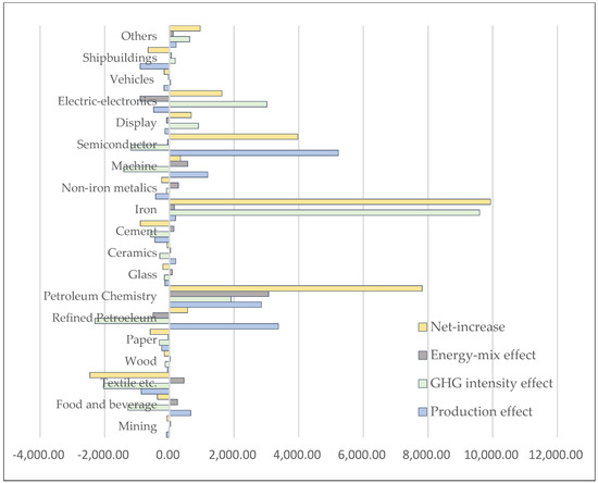
Figure 1.
Decomposition results of LMDI.
This analysis is conducted following two assumptions:
- (1)
- Industrial growth per employed population is the same in 2016 and 2019.
- (2)
- Increase in GHG emissions per employed population is the same in 2016 and 2019.
With these two assumptions, regional industrial growth (production effect) depends on the growth rate of each regional competition characteristic. In addition, each technological progress (GHG intensity effect) depends on the industry’s growth rate. This study sets the shift-share model as follows. The growth of an industry in a specific region is developed following (4). The definitions of the characters are given in (4) notes.
- .
- .
- .
The growth of an industry in a particular region is decomposed into three factors, which are given in (5). The total economic growth effect, industrial structure effect, and regional competition effect are extracted.
- .
- .
- .
This study obtains each industry’s GDP and employment by LRGs as GHG inventory from 2016 to 2019. The economic growth rates in each industry are also shown. By the assumptions, the shift-share equation is represented as (6) through GHG emission quantity unit.
.
With regard to the LMDI analysis above, this study already provides the three effects. In this part, this study excludes the energy mix effect because external suppliers control the variable that production agents cannot adjust. Equation (7) focuses on the production effect presented by an economic variable and the GHG intensity effect indicating technological progress, i.e., and .
Regarding the shift-share analysis, this study already provides the three effects in (6). Except for national-wide growth as a controlled external variable, each industry growth effect () offers technological progress (). The regional competition effect offers regional economic growth (). Equation (8) is the same as (6) in terms of equality.
Economic effects are grouped between economic variables to compensate for the regional and industrial effects on GHG emission abatement performance. Technological effects are grouped between technological variables. The effects derived from LMDI are converted into adjusted data. They are divided into individual economic and technological variables, 17 LRGs 19 industries. Unidentified geographical distinctive traits or distinctive technological traits are arranged as in (9).
A scatter plot on the coordinate plane is drawable, as shown in the following Equation (10). This study defines as Economic Local Share Effect (ELSE) with a horizontal axis and as Industrial GHG Intensity Effect (IGIE) with a vertical axis.
3.4. Classification of Industrial Sectors
To measure the status of each industrial sector, a decoupled model was set on the coordinate plane. This categorization divides the effects of direction into four different situations for decision-makers who manage GHG emission performance. Area (A), both desirables, shows the economic growth of a detailed industry is increasing, and GHG intensity is decreasing. Area (B), economically desirable, shows the economic growth of a detailed industry sector increasing. However, GHG intensity is increasing. Area (C), both undesirables, shows the economic growth of a detailed industry is decreasing and GHG intensity is increasing. Area (D), technological desirable, shows the economic growth of a detailed industry is declining. However, GHG intensity decreases, as shown in Figure 2.
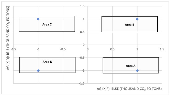
Figure 2.
Classification coordinate of industrial sectors.
The presence of both desirables (A) does not indicate the highest advantage for GHG neutrality; instead, it means that a dilemma exists between stakeholders. Similarly, the presence of both undesirables (C) do not indicate the least advantage for GHG neutrality; rather, it means that a dilemma exists between stakeholders. From the simple human-welfare perspective, the situations are desirable and undesirable. However, stakeholders should choose the opposite decision for carbon neutrality. Instead, technological desirable (D) means the most advantage for carbon neutrality, although it means ineffectiveness for the short-term attainment of human welfare. Economic desirable (B) indicates the least advantage for GHG neutrality, but it means effectiveness in the short-term achievement of human welfare. Whether (A) and (C) can abate GHG is unpredictable. However, whether (B) and (D) can achieve the GHG abatement target is predictable. The inner two stakeholders who desire economic growth or technical progress in GHG intensity evaluate their performance similarly in (A) and (C). By contrast, inner stakeholders evaluate their performance oppositely in (B) and (D). An individual LRG faces a different situation with the hypothesis. It categorizes four positions by 17 LRGs. Moreover, it suggests five representative detailed MM industries by an LRG, chosen from the distance of a zero-point as follows. Furthermore, through the ratio of both effects in a particular MM industry, the aspect of carbon neutrality that each LRG faces is shown in detail.
More importantly, this decoupled classification can derive the following policy implications. At the local level, decision-makers should consider regional characteristics because the importance of industries that affect carbon emissions varies across regions. When presenting carbon neutrality strategies by industry, it is unnecessary to present each region’s industry. The entire country can only present a uniform carbon-neutral process for each industry. This analysis also suggests the following strategies:
- (A)
- Both Desirables: These industries can take a strategy to continuously expand investment in carbon-reducing technologies through R&D so that the (+) utility made by the economic growth effect can guarantee a continuous decline in carbon concentration in production.
- (B)
- Economic Desirable: These industries are not currently shifting the (+) utility received from the economic growth effect to carbon-reducing technological advances. However, with the utility due to economic growth, they can improve reduction performance by taking a radical investment strategy to acquire R&D or carbon emission rights.
- (C)
- Both Undesirables: These industries reduce GHG emissions through virtual windfall profiles in GHG emissions. However, as the ability to change the direction of carbon concentration effects through technological progress is reduced, strategically, it is possible to change the industry itself or to attract external technologies or cooperate if the industry is maintained.
- (D)
- Technological Desirable: These industries can use strategies to maintain and sustain carbon-reducing R&D through external investment. They can partially reduce the industry’s risk through windfall propitiation and advance GHG emission reduction processes.
With these implications, the results of the classification of each industrial sector will be discussed thoroughly in the following section.
4. Results
The ELSE and IGIE effects of each LRG as GHG emission performance are shown in Figure 3. No regions in Area (C) show both undesirables. Ulsan, Daegu, Gangwon, and Jeju are located in Area (A), and show both desirables. Daegu, Gangwon, and Jeju show that IGIEs are enough to offset the ELSE. However, Ulsan shows that IGIEs are not enough to offset the ELSE. Therefore, the organizations should consider what MM industries are elected and concentrate on carbon neutrality and how agents manage the trade-off relationship between both effects. Figure 3 supplements them.
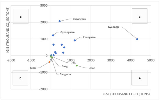
Figure 3.
Results of classification of Korean LRGs.
Seoul is located in Area (D), which is technologically desirable. Seoul shows the result desirable for the total abatement of GHG emissions. Both effects can offset performance derived from the energy mixture effect, and approaching carbon neutrality can be closest to others in the MM industry. However, whether the ELSE performance is derived from economic withdrawal or IGIE increase occurring out of MM industries is not certain. The other LRGs are located in Area (B), which is economically desirable. They show conventional economic growth, that is, more carbon consumption in production. IGIE in Gyeonggi shows the potential to convert the direction. The others are not remarkable in the conversion. They should consider the conversion to carbon neutrality urgently.
The total quantity of GHG change effects in each province is shown above. Each analysis is too scattered to understand, so a comprehensive analysis should be conducted to manage national GHG inventory in the future. Motivation and concentration are vital for carbon neutrality. For the objective, this study conducted additional analyses of the effects between region and country with detailed MM industries.
This study chose five significant industries that influence the performance of GHG abatement. The commonalities and differences between the effects of carbon emissions in local industries were revealed. Table 4 shows the number of observations in five industries with significant impacts on the GHG emission performance of 17 LRGs.
Table 4.
Observations of five main industries influencing GHG emission performance.
Suppose the classification of the reduction target industry is reasonable. In this case, the commonalities and differences in GHG emissions by LRGs are revealed clearly. As commodities, the petroleum chemistry industry is observed 16 times in Korean LRGs as one of the five major industries influencing GHG emission change. The iron industry is shown 15 times, and the electron/-electronics industry is shown 13 times. Wood, non-iron metallics, and vehicles are not observed. This finding implies that the abatement performance in those industries is comparatively homogenous compared with other industries. These industries depend on the national performance of economic growth and GHG technological progress rather than their LRG performance.
Some differences are noted between LRGs. The food and beverage industry is one of the five major industries in five LRGs, namely, Sejong, Gangwon, Chungbuk, Jeonbuk, and Jeju. These LRGs are far from the metropolitan centers but are not also metropolitan in Korea. The changes in the GHG emission performance of the refined petroleum and shipbuilding industries show that they follow the geographical and economic scales and locations near the seashore. The machine industry is in inland LRGs, demonstrated by the change in its GHG emission performance. When discussing the individual performances for carbon neutrality, the BAU of each regional industry of the base year should be considered. As shown in each second graph of each analysis, the ratios of ELSE and IGIE are considered together. This is due to the heterogeneity of LRGs. Then, each performance of local industries can be interpreted comprehensively.
Finally, a specific performance index that is adjusted according to the size of each LRG is necessary. For carbon neutrality, how much hosts should weigh on 19 industries in each region is analyzed. It refers to the priority of choice and concentration for the GHG industry from the local level. The index calculation is as follows. In each region, it calculates how much other industries account for, letting a specific industry that influences the most significant impact on carbon emission performance be 100. The other industries are calculated from the weight of the maximum 100. The following index result is helpful for the national–regional carbon neutrality objective (Table 5). Furthermore, each location of local industries in categories (A)–(D) is presented in Table 6. If the location change is remarkable, GHG abatement strategies should be established at the local level. If not, a unified strategy should be established at the national level. Like the analysis in Table 4, the weight of industries from a local level comparably shows heterogeneity in GHG emissions. However, the locations are comparably similar to LRGs. In the 323 cases, the difference is shown three times in semiconductors and vehicles in Sejong, Gangwon, and Jeju.
Table 5.
Weight of each MM industry in 17 LRGs.
Table 6.
Location of each MM industry in 17 LRGs.
5. Conclusions
This study aimed to investigate two research questions: whether urban economic structure interrelates with GHG emission and whether heterogeneous industrial structure by regions indeed affects local carbon emission. To approach this research question, this study adopted two methodologies, LMDI and shift-share analysis. The LMDI method is widely used to decompose the effect, and shift-share analysis can quantify the relationship between the industry and regional characteristics.
The main theoretical contribution of this study is that it considers the local heterogeneity in assessing the condition of GHG emissions. Most of the previous studies do not sufficiently consider the fundamental aspect of regional heterogeneity. For this, with empirical research, this study proves that heterogeneous urban economic structure interacts with each element of GHG emission, which demonstrates that carbon abatement aspects are indeed heterogeneous by urban spatial production. However, there are also some limitations of this study. First, this study started from the assumption that two essential variables, economic growth and technological change, have a trade-off. However, these trade-offs happen mostly in medium- and long-term dimensions, while this study used limited data, from 2016 to 2019, because of data availability. In addition, the question of data validity is also another limitation of this study. About 70,000 pieces of data were collected from the shift-share analysis. However, the LMDI analysis uses sampled data, with the research assuming that the data are the same. Therefore, further analysis using long-term and more valid data should proceed.
Some interesting points were also found in the Korean mining and manufacturing industry analysis. It was proved that industrial structure causes GHG emissions in each industry. For example, the iron and petroleum chemistry industries show remarkable (+) quantities in economic growth and technological progress. In contrast, the semiconductor industry shows the opposite direction in two effects on employment. Additionally, geographical differences also proved to influence GHG emission status. Based on the assumptions that industrial growth and GHG emission increase per employed population are the same in 2016 and 2019, the results show a significant difference between LRGs in GHG emission performances by their industrial structure. For example, inland metropolitan regions show GHG emission decrease in the textile industry. However, the machine industry and semiconductor industry offset ELSE and IGIE. Additionally, the IGIE per ELSE ratio of the machine is more than that of the semiconductor industry. In contrast, inland non-metropolitan and Jeju in LRGs show the GHG emission decrease in the food and beverage industry. The cement industry shows great occupation in Chungbuk and Gangwon. Gangwon is the only LRG, including the mining industry in five major industries, and both effects show (−) direction. Regarding petroleum chemistry, LRGs near the seashore show a remarkable GHG emission increase. Although the occupation of refined petroleum is remarkable, it seems that it is not possible to offset the (+) ELSE by the (−) IGIE. Moreover, the shipbuilding industry in the five industries is observed in three southern provinces near the seashore.
In brief, economic growth and technological progress in GHG emission aspects are heterogenous by LRGs, caused by geographical territorial advantage and disadvantage. This means that policymakers should decide which sector to focus on to achieve carbon neutrality. Additionally, the dilemmas between stakeholders in carbon neutrality should be adjusted with a well-designed governance system [51,52,53]. In achieving carbon neutrality, there is a dilemma [54] pertaining to the conflicts between stakeholders that can emerge or pursue different goals in achieving carbon neutrality. The existing governance system led by central government does not properly consider the differences and heterogeneity by industry sectors and regions. However, this study reveals the performance of GHG reduction is distinct by the region and industry. Huge efforts should be made to build a more detailed governance system that could encompass each different decision maker in regions and industry. The assessment method provided in this study, four categorizations, could be used to set effective strategies for achieving carbon neutrality. More precise and effective methods should be developed through following research.
Author Contributions
All authors conceived, designed, and implemented the study. H.K.: data curation, formal analysis, investigation, and writing; H.D.Z.: investigation, and writing. All authors have read and agreed to the published version of the manuscript.
Funding
This work is supported by the Korea Agency for Infrastructure Technology Advancement (KAIA) grant funded by the Ministry of Land, Infrastructure and Transport (Grant 21DEAP-B158906-02).
Data Availability Statement
All the data used in this study can be found on the website of Korea Energy Agency (KEA), Bank of Korea (BOK), and Statistics Korea (KOSTAT).
Acknowledgments
This paper is conducted based on the results of Hyungsu Kang’s doctoral dissertation, “The Analysis of the Local Industrial Structure in Korea toward Carbon Neutrality”.
Conflicts of Interest
The authors declare no conflict of interest. The funders had no role in the design of the study; in the collection, analyses, or interpretation of data; in the writing of the manuscript, or in the decision to publish the results.
References
- Bitan, A. The methodology of applied climatology in planning and building. Energy Build. 1988, 11, 1–10. [Google Scholar] [CrossRef]
- Eliasson, I. Infrared thermography and urban temperature patterns. Int. J. Remote Sens. 1992, 13, 869–879. [Google Scholar] [CrossRef]
- De Ridder, K.; Adamec, V.; Bañuelos, A.; Bruse, M.; Bürger, M.; Damsgaard, O.; Dufek, J.; Hirsch, J.; Lefebre, F.; Pérez-Lacorzana, J.M.; et al. An integrated methodology to assess the benefits of urban green space. Sci. Total Environ. 2004, 334, 489–497. [Google Scholar] [CrossRef] [PubMed]
- Ngowi, A.B. Creating competitive advantage by using environment-friendly building processes. Build. Environ. 2001, 36, 291–298. [Google Scholar] [CrossRef]
- Heidt, V.; Neef, M. Benefits of urban green space for improving urban climate. In Ecology, Planning, and Management of Urban Forests; Springer: New York, NY, USA, 2008; pp. 84–96. [Google Scholar]
- Artmann, M.; Inostroza, L.; Fan, P. Urban sprawl, compact urban development and green cities. How much do we know, how much do we agree? Ecol. Indic. 2019, 96, 3–9. [Google Scholar] [CrossRef]
- Heikinheimo, V.; Tenkanen, H.; Bergroth, C.; Järv, O.; Hiippala, T.; Toivonen, T. Understanding the use of urban green spaces from user-generated geographic information. Landsc. Urban Plan. 2020, 201, 103845. [Google Scholar] [CrossRef]
- Opschoor, H. Local sustainable development and carbon neutrality in cities in developing and emerging countries. Int. J. Sustain. Dev. World Ecol. 2011, 18, 190–200. [Google Scholar] [CrossRef]
- Hussain, T.; Abbas, J.; Wei, Z.; Nurunnabi, M. The effect of sustainable urban planning and slum disamenity on the value of neighboring residential property: Application of the hedonic pricing model in rent price appraisal. Sustainability 2019, 11, 1144. [Google Scholar] [CrossRef]
- Tozer, L.; Klenk, N. Discourses of carbon neutrality and imaginaries of urban futures. Energy Res. Soc. Sci. 2018, 35, 174–181. [Google Scholar] [CrossRef]
- Rauland, V.; Newman, P. Decarbonising Cities: Mainstreaming Low Carbon Urban Development; Springer: Berlin/Heidelberg, Germany, 2015. [Google Scholar]
- Bouzarovski, S.; Haarstad, H. Rescaling low-carbon transformations: Towards a relational ontology. Trans. Inst. Br. Geogr. 2019, 44, 256–269. [Google Scholar] [CrossRef]
- Torrens, J.; Westman, L.; Wolfram, M.; Broto, V.C.; Barnes, J.; Egermann, M.; Ehnert, F.; Frantzeskaki, N.; Fratini, C.F.; Håkansson, I.; et al. Advancing urban transitions and transformations research. Environ. Innov. Soc. Transit. 2021, 41, 102–105. [Google Scholar] [CrossRef]
- Qin, L.; Kirikkaleli, D.; Hou, Y.; Miao, X.; Tufail, M. Carbon neutrality target for G7 economies: Examining the role of environmental policy, green innovation and composite risk index. J. Environ. Manag. 2021, 295, 113119. [Google Scholar] [CrossRef] [PubMed]
- Salvia, M.; Reckien, D.; Pietrapertosa, F.; Eckersley, P.; Spyridaki, N.A.; Krook-Riekkola, A.; Olazabal, M.; Hurtado, S.D.G.; Simoes, S.G.; Geneletti, D.; et al. Will climate mitigation ambitions lead to carbon neutrality? An analysis of the local-level plans of 327 cities in the EU. Renew. Sustain. Energy Rev. 2021, 135, 110253. [Google Scholar] [CrossRef]
- Herrador, M.; de Jong, W.; Nasu, K.; Granrath, L. Circular economy and zero-carbon strategies between Japan and South Korea: A comparative study. Sci. Total Environ. 2022, 820, 153274. [Google Scholar] [CrossRef] [PubMed]
- Hyungna, O.H.; Hong, I.; Ilyoung, O.H. South Korea’s 2050 Carbon Neutrality Policy. East Asian Policy 2021, 13, 33–46. [Google Scholar]
- Tae, S.; Shin, S. Current work and future trends for sustainable buildings in South Korea. Renew. Sustain. Energy Rev. 2009, 13, 1910–1921. [Google Scholar] [CrossRef]
- Pan, H.; Jessica, P.; Le, Z.; Cong, C.; Carla, F.; Elisie, J.; Helena, N.; Georgia, D.; Brian, D.; Zahra, K. Understanding interactions between urban development policies and GHG emissions: A case study in Stockholm Region. Ambio 2020, 49, 1313–1327. [Google Scholar]
- LI, J. Decoupling urban transport from GHG emissions in Indian cities—A critical review and perspectives. Energy Policy 2011, 39, 3503–3514. [Google Scholar] [CrossRef]
- Lau, L.C.; Lee, K.T.; Mohamed, A.R. Global warming mitigation and renewable energy policy development from the Kyoto Protocol to the Copenhagen Accord—A comment. Renew. Sustain. Energy Rev. 2012, 16, 5280–5284. [Google Scholar] [CrossRef]
- Satterthwaite, D. The implications of population growth and urbanization for climate change. Environ. Urban. 2009, 21, 545–567. [Google Scholar] [CrossRef]
- Cai, B.; Cui, C.; Zhang, D.; Cao, L.; Wu, P.; Pang, L.; Zhang, J.; Daie, C. China city-level greenhouse gas emissions inventory in 2015 and uncertainty analysis. Appl. Energy 2019, 253, 113579. [Google Scholar] [CrossRef]
- Vallés-Giménez, J.; Zárate-Marco, A. A dynamic spatial panel of subnational GHG emissions: Environmental effectiveness of emissions taxes in Spanish regions. Sustainability 2020, 12, 2872. [Google Scholar] [CrossRef]
- Aydin, C.; Esen, Ö. Reducing CO2 emissions in the EU member states: Do environmental taxes work? J. Environ. Plan. Manag. 2018, 61, 2396–2420. [Google Scholar] [CrossRef]
- Witte, D. Business for Climate: A Qualitative Comparative Analysis of Policy Support from Transnational Companies. Glob. Environ. Politics 2020, 20, 167–191. [Google Scholar] [CrossRef]
- Yoo, J.-I.; Lee, D.-H.; Cheong, Y.-K.; Kim, S.-H.; Jeong, Y.-S.; Lee, D.-H.; Park, S.-K.; Kim, M.-J. Methodological approaches for estimating regional emission values using national greenhouse gas inventory: A case study of the Republic of Korea. Greenh. Gases Sci. Technol. 2021, 11, 539–553. [Google Scholar] [CrossRef]
- Mckitrick, R. A derivation of the marginal abatement cost curve. J. Environ. Econ. Manag. 1999, 37, 306–314. [Google Scholar] [CrossRef]
- Battese, G.E.; Coelli, T.J. A model for technical inefficiency effects in a stochastic frontier production function for panel data. Empir. Econ. 1995, 20, 325–332. [Google Scholar] [CrossRef]
- Kumbhakar, S.C.; Lovell, C.A.K. Stochastic Frontier Analysis; Cambridge University Press: Cambridge, UK, 2003. [Google Scholar]
- Sun, J.; Du, T.; Sun, W.; Na, H.; He, J.; Qiu, Z.; Yuan, Y.; Li, Y. An evaluation of greenhouse gas emission efficiency in China’s industry based on SFA. Sci. Total Environ. 2019, 690, 1190–1202. [Google Scholar] [CrossRef]
- Hoffmann, V.H.; Busch, T. Corporate carbon performance indicators: Carbon intensity, dependency, exposure, and risk. J. Ind. Ecol. 2008, 12, 505–520. [Google Scholar] [CrossRef]
- Roberts, J.T.; Grimes, P.E. Carbon intensity and economic development 1962–1991, A brief exploration of the environmental Kuznets curve. World Dev. 1997, 25, 191–198. [Google Scholar] [CrossRef]
- Scarlat, N.; Prussi, M.; Padella, M. Quantification of the carbon intensity of electricity produced and used in Europe. Appl. Energy 2022, 305, 117901. [Google Scholar] [CrossRef]
- Andersson, F.N.G.; Karpestam, P. CO2 emissions and economic activity: Short-and long-run economic determinants of scale, energy intensity and carbon intensity. Energy Policy 2013, 61, 1285–1294. [Google Scholar] [CrossRef]
- Doda, B. Tales from the tails: Sector-level carbon intensity distribution. Clim. Chang. Econ. 2018, 9, 1850011. [Google Scholar] [CrossRef]
- Reitler, W.; Rudolph, M.; Schaefer, H. Analysis of the factors influencing energy consumption in industry: A revised method. Energy Econ. 1987, 9, 145–148. [Google Scholar] [CrossRef]
- Rozenberg, J.; Davis, S.J.; Narloch, U.; Hallegatte, S. Climate constraints on the carbon intensity of economic growth. Environ. Res. Lett. 2015, 10, 095006. [Google Scholar] [CrossRef]
- Kim, S.; Jung, K. LMDI decomposition analysis for GHG emissions of Korea’s manufactring industry. Environ. Resour. Econ. Rev. 2011, 20, 229–254. [Google Scholar]
- Ozturk, I.; Majeed, M.T.; Khan, S. Decoupling and decomposition analysis of environmental impact from economic growth: A comparative analysis of Pakistan, India, and China. Environ. Ecol. Stat. 2021, 28, 793–820. [Google Scholar] [CrossRef]
- Ang, B.W. LMDI decomposition approach: A guide for implementation. Energy Policy 2015, 86, 233–238. [Google Scholar] [CrossRef]
- Park, N.-B.; Shim, S.H. Decomposition Analysis of Energy Consumption and GHG Emissions by Industry Classification for Korea’s GHG Reduction Targets. Environ. Resour. Econ. Rev. 2015, 24, 189–224. [Google Scholar] [CrossRef]
- Sato, K. The ideal log-change index number. Rev. Econ. Stat. 1976, 58, 223–228. [Google Scholar] [CrossRef]
- Sheinbaum, C.; Ozawa, L.; Castillo, D. Using logarithmic mean Divisia index to analyze changes in energy use and carbon dioxide emissions in Mexico’s iron and steel industry. Energy Econ. 2010, 32, 1337–1344. [Google Scholar] [CrossRef]
- Wang, M.; Feng, C. Using an extended logarithmic mean Divisia index approach to assess the roles of economic factors on industrial CO2 emissions of China. Energy Econ. 2018, 76, 101–114. [Google Scholar] [CrossRef]
- Jung, S.; An, K.-J.; Dodbiba, G.; Fujita, T. Regional energy-related carbon emission characteristics and potential mitigation in eco-industrial parks in South Korea: Logarithmic mean Divisia index analysis based on the Kaya identity. Energy 2012, 46, 231–241. [Google Scholar] [CrossRef]
- Wang, Q.; Song, X. How UK farewell to coal–Insight from multi-regional input-output and logarithmic mean divisia index analysis. Energy 2021, 229, 120655. [Google Scholar] [CrossRef]
- Kim, S. LMDI decomposition analysis of energy consumption in the Korean manufacturing sector. Sustainability 2017, 9, 202. [Google Scholar] [CrossRef]
- Yu, S.; Kim, D. Changes in Regional Economic Resilience after the 2008 Global Economic Crisis: The Case of Korea. Sustainability 2021, 13, 11392. [Google Scholar] [CrossRef]
- Bao, C.; Liu, R. Electricity consumption changes across China’s provinces using a spatial shift-share decomposition model. Sustainability 2019, 11, 2494. [Google Scholar] [CrossRef]
- Cogan, D.G. Corporate Governance and Climate Change: Making the Connection; Ceres, Inc.: Boston, MA, USA, 2006. [Google Scholar]
- Barnett, M.L.; Salomon, R.M. Beyond dichotomy: The curvilinear relationship between social responsibility and financial performance. Strateg. Manag. J. 2006, 27, 1101–1122. [Google Scholar] [CrossRef]
- Stuebs, M.; Sun, L. Corporate governance and social responsibility. Int. J. Law Manag. 2015, 57, 38–52. [Google Scholar] [CrossRef]
- Cornell, B. ESG Investing: Conceptual Issues. J. Wealth Manag. 2020, 23, 61–69. [Google Scholar] [CrossRef]


Publisher’s Note: MDPI stays neutral with regard to jurisdictional claims in published maps and institutional affiliations. |
© 2022 by the authors. Licensee MDPI, Basel, Switzerland. This article is an open access article distributed under the terms and conditions of the Creative Commons Attribution (CC BY) license (https://creativecommons.org/licenses/by/4.0/).