Synchronizing Torque-Based Transient Stability Index of a Multimachine Interconnected Power System

Abstract

Newly developed tools and techniques are continuously established to analyze and monitor power systems’ transient stability limits. In this paper, a model-based transient stability index for each generator is proposed from the synchronizing torque contributions of all other connected generators in a multi-machine interconnected power system. It is a new interpretation of the generator’s synchronizing torque coefficient (STC) in terms of electromechanical oscillation modes to consider the synchronizing torque interactions among generators. Thus, the system operator can continuously monitor the system’s available secured transient stability limit in terms of synchronizing torque more accurately, which is helpful for planning and operation studies due to the modal based index. Furthermore, the popular transient stability indicator critical clearing time (CCT), and the traditionally determined synchronizing torque values without other generator contributions, are calculated to verify and compare the performance of the proposed transient stability index. The simulations and test result discussions are performed over a western system coordinating council (WSCC) 9-bus and an extensive New England 68-bus large power test system cases. The open-source power system analysis toolbox (PSAT) on the MATLAB/Simulink environment is used to develop, simulate, validate and compare the proposed transient stability index.

1. Introduction

Power system studies worldwide are concerned about the increasing complexity of power systems and their consequences. Due to environmental and economic constraints, most power systems are close to their static and dynamic stability limits, including a lack of transmission expansion, increased power consumption, and a substantial distance between power plants and loads. Furthermore, because power is transferred from generation surplus areas to deficit areas, deregulating energy markets causes transmission congestion. Consequently, the distance between the normal operating range and the power system’s critical stability limit keeps narrowing. If the system is subjected to anomalous conditions or disturbances and is not treated on time, the system experiences cascaded events that might result in a blackout. The references [1,2,3] detail the major blackouts and cascaded emergencies in the previous decade, with their root causes and consequences. Therefore, accurate monitoring of the system’s transient stability is critical and can help the system operator to determine system states following a significant disturbance (e.g., faults, loss of loads).

A power system’s transient stability is related to its ability to remain synchronized after being subjected to a large disturbance [4]. Different techniques have been employed in the transient stability analysis literature, but most have drawbacks. The time-domain simulation is a reliable method, where power system dynamic models are represented by differential equations and solved numerically at each instant by applying contingencies or faults at a specified period. Hence, this method requires high computation for solving nonlinear differential-algebraic equations due to the bulk power systems’ large dimensionality and nonlinearity [5]. However, model-based direct methods are derived to determine the quantitative information of the system’s stability based on the ability to absorb fault-on energy during the post-fault period. The Lyapunov stability-based transient energy function (TEF) methods calculate the kinetic energy stored on the rotor during fault-on and the potential energy released during the post-fault period [6]. Later, extended equal area criterion (EEAC) based methods are introduced to determine power systems’ transient stability based on the equivalent single-machine infinite bus (SMIB) system’s characteristics [7,8]. The limited scalability and conservativeness limit the direct methods; however, some advanced hybrid methods have been developed by combining both time-domain and $TEF$ methods to improve previous methods’ performance [9,10,11]. Recently, the bulk availability of measured data and fast computations has reignited the interest in advanced machine learning tools, such as decision trees [12], neural networks [13], and fuzzy knowledge-based systems [14] for measurement-based transient stability analysis, and the research area keeps expanding at a fast pace with new algorithms. In addition to that, the measured system state variables are used to analyze power systems’ stability through the estimated synchronizing torque values [15,16,17,18]. However, the model-based transient stability analysis through generators’ synchronizing torques is still the least explored research area.

The synchronizing torque is an electrical torque component produced by interacting stator windings and a fundamental air-gap flux component of the synchronous generator defined in [19]. The post-fault power network’s restoring or synchronizing torque availability can analyze a power system’s transient stability. During disturbances, the generators’ magnetic fields’ accumulated energy ensures precise immediate power support, and these magnetic fields are distributed according to the synchronizing torque coefficients (STC) matrix of the multimachine interconnected power system. Thus, the larger synchronizing torque values indicate a more substantial stability region through stable initial rotor angle deviations. However, the smaller synchronizing torque values diverge the rotor angles with the power system’s nonoscillatory instability [20]. Traditionally, each machine’s synchronizing torque calculations were used to determine the system’s immediate transient stability information during disturbances [20,21]. Recently, the paper [22] investigated the impact of generator location and reactive power output on the generator rotor speed deviations from the STC matrix by considering the multimachine Heffron–Phillips model and the network admittance matrix.

The synchronizing torque interactions among the generators in a power system are carried through the rotor oscillations, and the corresponding synchronizing torque values vary with the respective generator contributions on the modes [15]. The traditional synchronizing torque is calculated by focusing on only one target generator and not including the contributions from the other generators over power system networks. Consequently, the corresponding transient stability information is obtained from the approximated SMIB system, which is inaccurately determined. This paper presents a new transient stability index that investigates the synchronizing torque contributions from other generators with the generators’ electromechanical interactions to improve the accuracy of the transient stability index of a multi-machine power system. From the modal analysis, the systems’ eigenvalues, eigenvectors, and participation factors are utilized to express a relationship between generators, and then the contributions from other generators are added to the traditional method. The new index accurately indicates dominant generators’ net synchronizing torque values and transient stability information of the system. However, the proposed method requires systems’ modal information and performs further calculations to determine the stability index.

The remaining sections of the paper are organized as follows. Section 2 deals with the background theory for developing a stability index comprising the STC matrix and the linearized models of the multimachine interconnected power system. The proposed transient stability index is derived in Section 3 with a detailed explanation of the general three-machine example case. In Section 4, the proposed index is verified and compared on a western system coordinating council (WSCC) 9-bus test system and a large New England 68-bus test system with simulation studies and discussions. Finally, Section 5 concludes the paper with future research directions.

2. Background Theory

The following sections discuss essential power system dynamic concepts required to derive and verify the proposed transient stability index. A multimachine power system’s synchronizing torques are derived first, then the general system stability remarks from the traditional synchronizing torque calculations are described. In addition, the conventionally used transient stability indicator, critical clearing time (CCT) is briefly explained, which is used to evaluate the performance of the proposed transient stability index.

2.1. STC Matrix from Linearized Models of Multimachine Power System

For a multimachine power system with $N_G$ machines without considering damping torques, the swing equation of the ith machine is defined by reducing the network admittance matrix into the machine’s internal node and operating point linearization around the equilibrium point as follows [20,23].

$$\Delta \dot{{\delta }_i}=\mathsf{\Omega }\Delta {\omega }_i$$

(1)

$$\dot{\Delta {\omega }_i}=\frac{1}{2H_i}\left(\Delta P_{mi}-K_{sii}\Delta {\delta }_i+\sum _{j=1,j\ne i}^{N_G}{K}_{sij}\Delta {\delta }_j\right)$$

(2)

Since $P_{mi}$ = constant and $2{H_i}^{-1}$ = ${M_i}^{-1}$, Equation (2) can be rearranged as follows

$$\dot{\Delta {\omega }_i}={M_i}^{-1}\left(-K_{sii}\Delta {\delta }_i+\sum _{j=1,j\ne i}^{N_G}{K}_{sij}\Delta {\delta }_j\right)$$

(3)

for i = 1, 2, …, $N_G$.

where

${\delta }_i$	ith machine rotor angle
${\delta }_j$	adjacent machine rotor angle
${\omega }_i$	ith machine rotor speed in pu
$P_{mi}$	ith machine mechanical power input
$H_i$	ith machine inertia constant
$\mathrm{\Omega }$	$=2\pi f$ is the per unit to radian conversion factor for the speed change.
$K_{sii}$	= ${\sum }_{j=1,j\ne 1}^{N_G}{E}_i{E}_j\left(B_{ij}\cos \left({\delta }_i-{\delta }_j\right)\right)-G_{ij}\sin \left({\delta }_i-{\delta }_j\right){|}_{\circ }$ are diagonal elements representing the total contribution of synchronizing torque from a machine to the network.
$K_{sij}$	= $E_i{E}_j\left(B_{ij}\cos \left({\delta }_i-{\delta }_j\right)\right)-G_{ij}\sin \left({\delta }_i-{\delta }_j\right){|}_{\circ }$ are off-diagonal elements representing the synchronizing torque interactions between the machines.
$E_i$	= constant voltage behind transient reactance of the machine i
$Y_{ii}$	$=G_{ii}+j{B}_{ii}$ diagonal element of the network’s short-circuit admittance matrix Y
$Y_{ij}$	$=G_{ij}+j{B}_{ij}$ off-diagonal element of the network’s short-circuit admittance matrix Y

The linearized multimachine power system’s state-space form can be represented as follows using Equations (1) and (3)

$$\begin{array}{c}\left[\begin{array}{c}\dot{\Delta {\delta }_i}\\ \dot{\Delta {\omega }_i}\end{array}\right]=A\left[\begin{array}{c}\Delta {\delta }_i\\ \Delta {\omega }_i\end{array}\right]\end{array}$$

(4)

where

A	= $\left[\begin{array}{cc}0& \mathsf{\Omega }I\\ M_i^{-1}{K}_s& 0\end{array}\right]$ is the system matrix,
$K_s$	= $\left[\begin{array}{ccc}-K_{s11}& \cdots & K_{s1N_G}\\ ⋮& \ddots & ⋮\\ K_{s{N}_{G}1}& \cdots & -K_{s{N}_G{N}_G}\end{array}\right]$ is the synchronizing torque coefficient (STC) matrix,
${M_i}^{-1}$	= $\left[\begin{array}{ccc}{M_1}^{-1}& \cdots & 0\\ ⋮& \ddots & ⋮\\ 0& \cdots & {M_{N_G}}^{-1}\end{array}\right]$ is the inertia constants of all synchronous machines in diagonal matrix form.

2.2. Synchronizing Torque and System Stability

The change in a synchronous machine’s electrical torque following a perturbation can be resolved into two components: synchronizing and damping torque coefficients, defined in [24] given in Equation (5).

$$\Delta T_e\left(t\right)=k_s\Delta \delta \left(t\right)+k_d\Delta \omega \left(t\right)$$

(5)

The synchronizing torque factor is in phase with the rotor angle perturbation $\Delta \delta \left(t\right)$, and $k_s$ indicates the synchronizing torque coefficient. The damping torque factor is in phase with the speed deviation $\Delta \omega \left(t\right)$, and the corresponding damping torque coefficient is $k_d$. These two torque coefficients indicate the system’s general stability characteristics from electric torque fluctuations. The positive $k_s$ and $k_d$ values ensure non-oscillatory and oscillatory stabilities, whereas negative values indicate the corresponding instabilities [24,25]. Traditionally, the synchronizing torque values of each generator ($K_{sTrad}$) in power systems are determined based on only the total synchronizing torque contributions from the generator to the network, which is obtained from the corresponding diagonal elements of the STC matrix in Equation (4) [22] through the SMIB system approximation. Therefore, the $K_{sTrad}$ values indicate individual generators’ approximate transient stability margin without considering other connected generator synchronizing torque interactions accurately.

2.3. Transient Stability Analysis through CCT

The CCT is the maximum duration a power system can tolerate in the fault-on state without becoming unstable before removing the fault. It should be noted that a CCT is specific to the fault’s type and location applied to the system, and it is explicitly stated that the normal clearing time is often much shorter than the CCT values. The CCT is a valuable metric for power system design and operation studies because it allows comparison of the severity of different conditions and effectiveness of numerous interventions such as generation dispatches, control modifications, or network reinforcements [26,27,28]. Thus, each generator’s transient stability limit can be determined by applying a three-phase fault near the generators and measuring the CCT values by varying the fault duration on the system.

3. Proposed Stability Index

The proposed transient stability index derivation is given in the first section with details. The index is then explained with a generalized three-machine test system case.

3.1. Derivation and Explanation

The time-domain response of states in linearized power system models can be expressed as the summation of n modes as shown in Equation (6).

$$\Delta x\left(t\right)=\sum _{h=1}^n\left(w_h^T\Delta x_0\right)v_h{e}^{{\lambda }_{h}t}$$

(6)

The term $w_h^T\Delta x_0$ with a contribution factor of left eigenvector $w_h$ represent the contribution of the initial state $\Delta x_0$ in the hth mode. The right eigenvector represented by $v_h$ denotes the mode shape and provides the participation of modes in each state, and ${\lambda }_h$ is the hth eigenvalue.

Using Equation (6), the ith machine’s rotor angle dynamic state variable can be represented in terms of eigenvectors for all n modes as shown in Equation (7).

$$\begin{array}{cc}\hfill \Delta {\delta }_i\left(t\right)& =\sum _{h=1}^n\left(w_h^T\Delta {\delta }_{0i}\right)v_h{e}^{{\lambda }_{h}t}\hfill \\ \hfill & =\sum _{h=1}^n{\Delta {\delta }_i}^h\left(t\right)\hfill \end{array}$$

(7)

where $\Delta {\delta }_{0i}$ indicates the ith machines’s initial rotor angle state variable, and the variable $\Delta {{\delta }_i}^h\left(t\right)$ represents the ith machine’s rotor angle change for the hth mode.

Therefore, the corresponding ith machine’s rotor speed change for the hth mode can be formulated from Equation (7) as follows.

$${\dot{\Delta \omega }}_i^h\left(t\right)={M_i}^{-1}\left(-K_{sii}{\Delta {\delta }_i}^h\left(t\right)+\sum _{j=1,j\ne i}^{N_G}{K}_{sij}{\Delta {\delta }_j}^h\left(t\right)\right)$$

(8)

Equation (8) consists of two components in terms of the STC matrix’s diagonal and off-diagonal elements. The off-diagonal element factor represents the other jth generator rotor angle interactions. Hence, the synchronizing torque contributions from jth generator on the ith generator can be accommodated by the eigenvector relationship between the rotor angle dynamic states of the generators expressed in Equation (7). The corresponding ith machine’s transient stability margin in terms of synchronizing torques, which includes the synchronizing torque contributions of the jth machine’s interactions for the hth mode, is accurately formulated in Equation (9).

$$\frac{{\dot{\Delta \omega }}_i^h\left(t\right)}{{\Delta {\delta }_i}^h\left(t\right)}={M_i}^{-1}\left(-K_{sii}+\frac{{\sum }_{j=1,j\ne i}^{N_G}{K}_{sij}{\Delta {\delta }_j}^h\left(t\right)}{{\Delta {\delta }_i}^h\left(t\right)}\right)$$

(9)

The traditional transient stability analysis through synchronizing torque coefficients considers the synchronizing torque interaction through the SMIB approximations. However, the proposed transient stability index in Equation (9) considers the synchronizing torque interactions from the other connected generators through the STC matrix elements and rotor angle time response for each mode obtained from the systems’ eigenvector modal information of the multimachine power system.

3.2. Example: A Generalized Three-Machine Interconnected System Case

The proposed transient stability index is explained on a three-machine interconnected power system $(N_G=3)$ with negligible damping torques. For an interconnected power system holding $N_G$ machines, there would be a $N_G-1$ set of electromechanical oscillation modes generated from swing equations, and the fundamental behavior of these modes is solely caught in the rotor angle and speed dynamic variables [20]. Hence, there are two electromechanical oscillation modes (n = 2) for the generalized three-machine example system case.

From Equation (7), the three machines’ rotor angle dynamic state’s time response can be independently split in terms of the rotor angle dynamic state variables of two modes formulated in Equation (10), calculated from the system’s eigenvector information through modal analysis.

$$\begin{array}{cc}\hfill \Delta {\delta }_1\left(t\right)& ={\Delta {\delta }_1}^1\left(t\right)+{\Delta {\delta }_1}^2\left(t\right)\hfill \\ \hfill \Delta {\delta }_2\left(t\right)& ={\Delta {\delta }_2}^1\left(t\right)+{\Delta {\delta }_2}^2\left(t\right)\hfill \\ \hfill \Delta {\delta }_3\left(t\right)& ={\Delta {\delta }_3}^1\left(t\right)+{\Delta {\delta }_3}^2\left(t\right)\hfill \end{array}$$

(10)

Therefore, the calculated values of each generator’s rotor angle dynamic states for each mode in Equation (10) can be used to determine the other generator’s synchronizing torque contribution factor for each mode separately.

For mode 1:

$$\begin{array}{cc}\hfill \frac{{\dot{\Delta \omega }}_1^1\left(t\right)}{{\Delta {\delta }_1}^1\left(t\right)}& ={M_1}^{-1}\left(-K_{s11}+K_{s12}\frac{{\Delta {\delta }_2}^1\left(t\right)}{{\Delta {\delta }_1}^1\left(t\right)}+K_{s13}\frac{{\Delta {\delta }_3}^1\left(t\right)}{{\Delta {\delta }_1}^1\left(t\right)}\right)\hfill \\ \hfill \frac{{\dot{\Delta \omega }}_2^1\left(t\right)}{{\Delta {\delta }_2}^1\left(t\right)}& ={M_2}^{-1}\left(K_{s21}\frac{{\Delta {\delta }_1}^1\left(t\right)}{{\Delta {\delta }_2}^1\left(t\right)}-K_{s22}++K_{s23}\frac{{\Delta {\delta }_3}^1\left(t\right)}{{\Delta {\delta }_2}^1\left(t\right)}\right)\hfill \\ \hfill \frac{{\dot{\Delta \omega }}_3^1\left(t\right)}{{\Delta {\delta }_3}^1\left(t\right)}& ={M_3}^{-1}\left(K_{s31}\frac{{\Delta {\delta }_1}^1\left(t\right)}{{\Delta {\delta }_3}^1\left(t\right)}+K_{s32}\frac{{\Delta {\delta }_2}^1\left(t\right)}{{\Delta {\delta }_3}^1\left(t\right)}-K_{s33}\right)\hfill \end{array}$$

(11)

For mode 2:

$$\begin{array}{cc}\hfill \frac{{\dot{\Delta \omega }}_1^2\left(t\right)}{{\Delta {\delta }_1}^2\left(t\right)}& ={M_1}^{-1}\left(-K_{s11}+K_{s12}\frac{{\Delta {\delta }_2}^2\left(t\right)}{{\Delta {\delta }_1}^2\left(t\right)}+K_{s13}\frac{{\Delta {\delta }_3}^2\left(t\right)}{{\Delta {\delta }_1}^2\left(t\right)}\right)\hfill \\ \hfill \frac{{\dot{\Delta \omega }}_2^2\left(t\right)}{{\Delta {\delta }_2}^2\left(t\right)}& ={M_2}^{-1}\left(K_{s21}\frac{{\Delta {\delta }_1}^2\left(t\right)}{{\Delta {\delta }_2}^2\left(t\right)}-K_{s22}++K_{s23}\frac{{\Delta {\delta }_3}^2\left(t\right)}{{\Delta {\delta }_2}^2\left(t\right)}\right)\hfill \\ \hfill \frac{{\dot{\Delta \omega }}_3^2\left(t\right)}{{\Delta {\delta }_3}^2\left(t\right)}& ={M_3}^{-1}\left(K_{s31}\frac{{\Delta {\delta }_1}^2\left(t\right)}{{\Delta {\delta }_3}^2\left(t\right)}+K_{s32}\frac{{\Delta {\delta }_2}^2\left(t\right)}{{\Delta {\delta }_3}^2\left(t\right)}-K_{s33}\right)\hfill \end{array}$$

(12)

Equations (11) and (12) provide the proposed transient stability margin of generators 1, 2, and 3 separately for modes 1 and 2, respectively. The proposed transient stability index considers the synchronizing torque contributions from other connected generators through the eigenvector information of each generator’s rotor angle dynamic states of each electromechanical oscillation mode.

4. Results and Discussions

The proposed transient stability index is verified and compared on two test case simulations; a small WSCC 9-bus test system with three synchronous generators, and a large New England 68-bus test system with 16 synchronous generators without considering exciter and governor dynamics. The test systems’ initial load bus information for the simulations are attached in the Appendix A, the static and dynamic data of the test systems are obtained from [29,30]. The MATLAB/Simulink-based open-source power system analysis toolbox (PSAT) is used for the simulations, and comparative studies [31].

The generators in the two test systems are modeled in subtransient machine models with negligible damping torque, and the loads are modeled with constant impedance models. The simulations and analysis are performed over a range of critical operating points obtained by a slowly varying load factor $\lambda$. The $\lambda$ vary the loads’ active and reactive power demands according to Equation (13) as follows [32].

$$\begin{array}{cc}\hfill P_L& =P_{L0}\left(1+\lambda \right)\hfill \\ \hfill Q_L& =Q_{L0}\left(1+\lambda \right)\hfill \end{array}$$

(13)

where $P_{L0}$ and $Q_{L0}$ are the initial real and reactive power levels of the loads on the test systems, respectively.

The variable $K_{sNew}^h$ indicates the generators’ proposed transient stability margins for the system’s hth mode. The popular time-domain transient stability indicator CCT verified the $K_{sNew}^h$ values, and the performance evaluation was conducted by comparing each generator’s $K_{sTrad}$ values determined from the system’s state matrix explained in Section 2.2. The $K_{sNew}^h$ and $K_{sTrad}$ values are plotted by its normalized values and CCT by its actual values for the following case studies.

4.1. The WSCC 9-Bus Test System

The $WSCC$ 9-bus test system’s eigenvalue analysis resulted in two electromechanical oscillation modes due to the three generator interactions. The system’s eigenvalues remained in the negative half of the s-plane, indicating a stable region of operating points over the range of $\lambda$ values. The proposed transient stability index in Equation (9) and the detailed expressions in Equations (11) and (12) for each modes are utilized to determine generators’ transient stability.

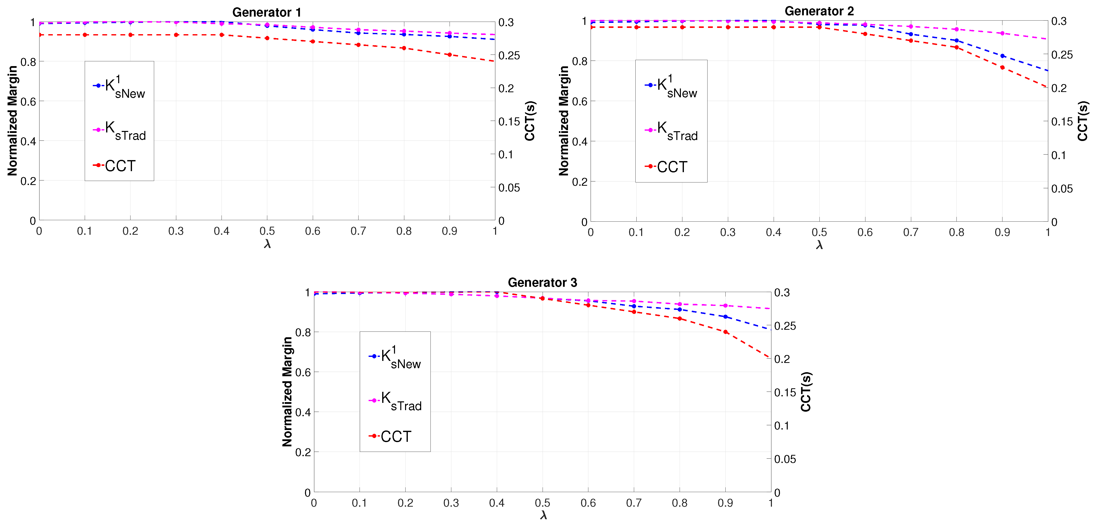
Figure 1 plotted the transient stability margin variation of the generators 1, 2 and 3 according to Equation (11) over the range of 0 to 1 values of $\lambda$. The $K_{sTrad}$, $K_{sNew}^1$ and CCT curves of three generators are decreasing over the increase in $\lambda$ values, indicating a reduction in the system’s overall transient stability and verifies the proposed transient stability index. Generator 1’s CCT values are slightly reduced from 0.28 s to 0.24 s and the normalized values of $K_{sTrad}$ and $K_{sNew}^1$ are slightly reduced to 0.93 and 0.87 over the range of $\lambda$ values. However, the CCT values of generator 2 and 3 are sharply reduced from 0.29 s and 0.30 s to 0.20 s, and the $K_{sNew}^1$ values of generator 2 and 3 follow a similar sharp reduction to 0.75 and 0.81, respectively. The $K_{sTrad}$ values of generators 2 and 3 show a slight decline in the normalized values to 0.90 and 0.91, respectively. Therefore, the $K_{sNew}^1$ values of generator 2 and 3 show a more accurate transient stability than the corresponding $K_{sTrad}$ values.

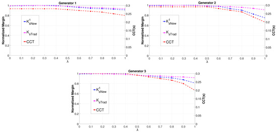
Figure 1. Transient stability margin of generators in WSCC 9-bus test system for mode 1.

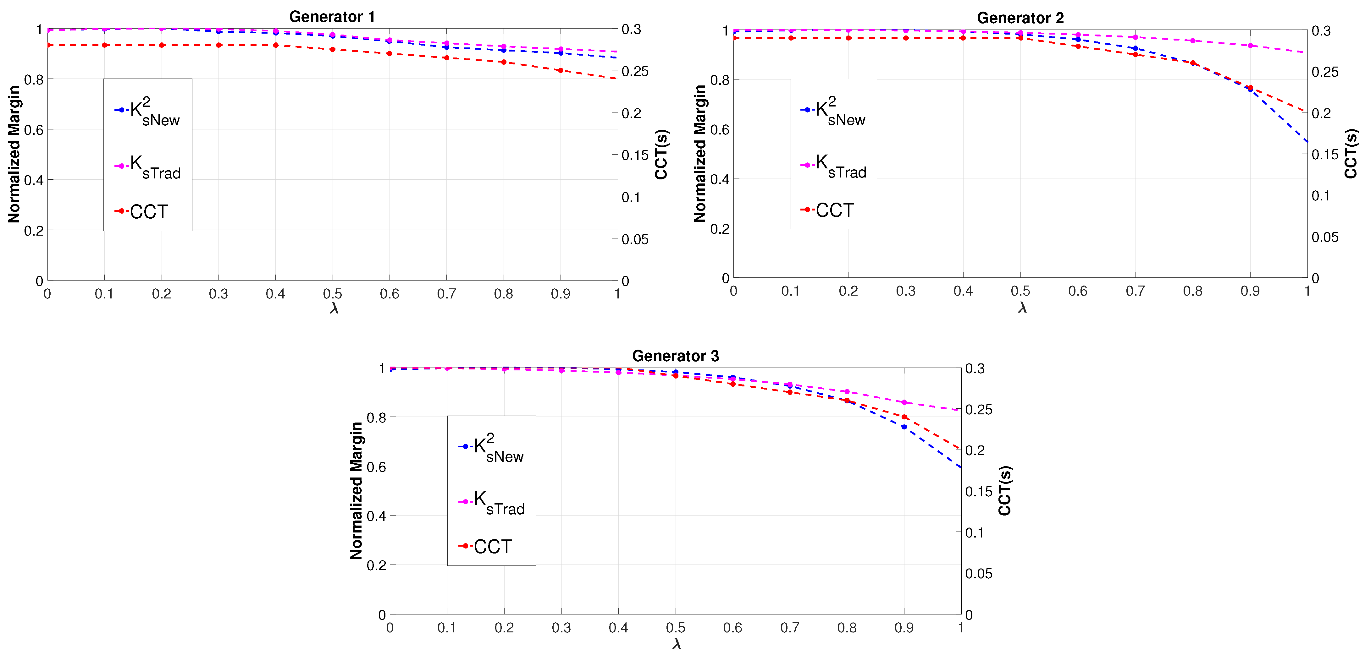
Figure 2 plots the transient stability margin variation of the generators 1, 2 and 3 according to the Equation (12) over the range of 0 to 1 values of $\lambda$. The $K_{sTrad}$, $K_{sNew}^2$ and CCT curves of three generators are decreased over the increase in $\lambda$ values, indicating a reduction in the system’s overall transient stability margin and verifying the proposed transient stability index. Generator 1’s CCT curve is slightly reduced from 0.28 s to 0.24 s and the normalized values of $K_{sTrad}$ and $K_{sNew}^2$ are slightly reduced to 0.90 and 0.88, respectively. However, the CCT values of generator 2 and 3 is sharply reduced from 0.29 s and 0.30 s to 0.20 s, and the $K_{sNew}^2$ values of generator 2 and 3 follow a similar sharp reduction to 0.54 and 0.59, respectively. The $K_{sTrad}$ values shows a slight decline in the normalized values to 0.90 and 0.82, respectively. Therefore, the $K_{sNew}^2$ values of generator 2 and 3 show a more accurate transient stability than the corresponding $K_{sTrad}$ values.

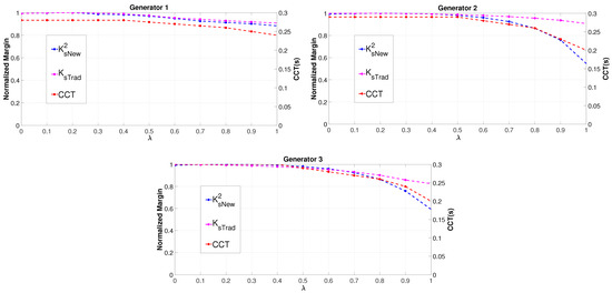
Figure 2. Transient stability margin of generators in WSCC 9-bus test system for mode 2.

4.2. The New England 68-Bus Test System

The New England 68-bus test system’s eigenvalue analysis resulted in 15 electromechanical oscillation modes due to the 16 generator interactions. The system’s eigenvalues remained in the negative half of the s-plane, indicating a stable region of operating points over the range of $\lambda$ values. According to the proposed transient stability index, 16 generators’ transient stability margins can be determined for all the 15 electromechanical modes. However, the critical transient stability of the system is primarily based on a few generators in the system. Therefore, the generators with decreasing CCT values over the rise of $\lambda$ values in the system are considered as critical generators. Therefore, the proposed transient stability index validation and comparison studies are performed only on these critical generators.

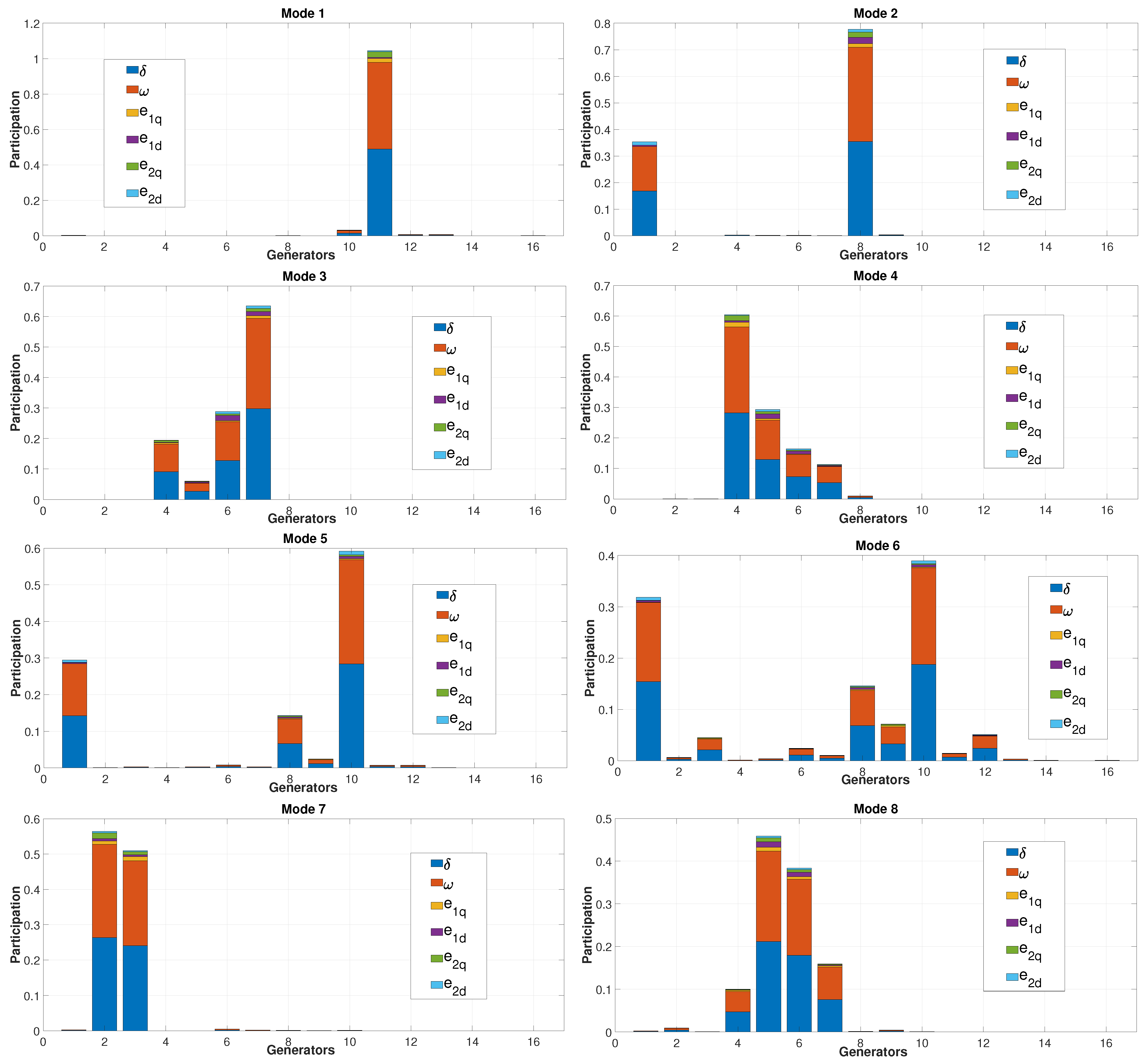
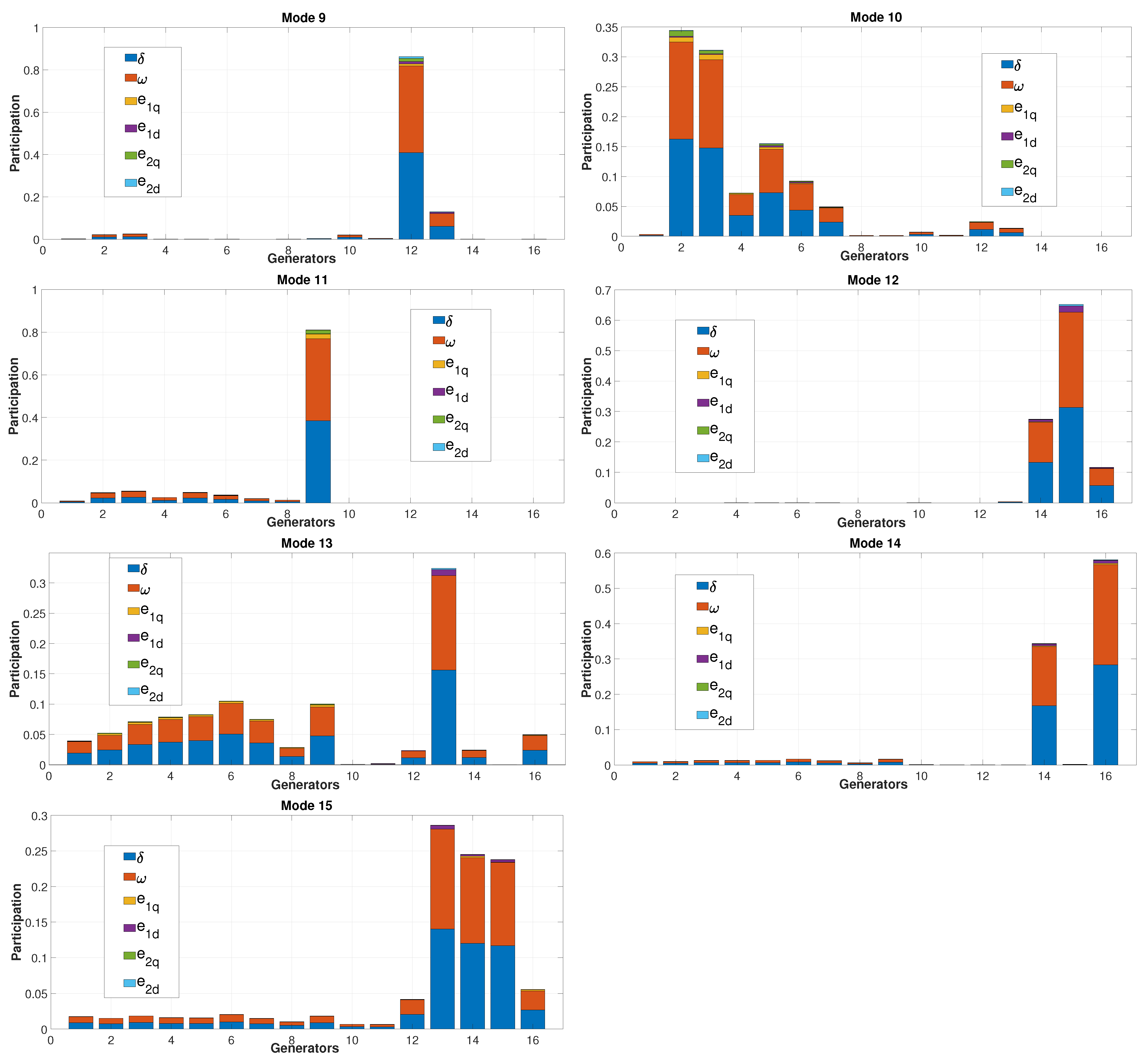
The proposed transient stability index calculates each generator’s transient stability based on the electromechanical modes excited on the system. Therefore, the system’s participation factor from eigenvalue analysis can be utilized to identify the associated generators and their contributions to each electromechanical mode separately shown in Figure 3. The X axis of each graph indicates the generator number and the Y axis represents the stacked participation value of the corresponding generator’s state variables $\delta$, $\omega$, $e_{1q}$, $e_{1d}$, $e_{2q}$ and $e_{2d}$ for subtransient machine models [23].

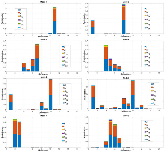
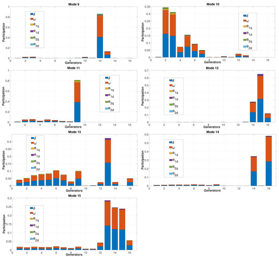
Figure 3. Participation factor information of electromechanical modes in New England 68-bus test system.

The generators and the corresponding associated electromechanical modes can also be identified from Figure 3, and it is summarized in Table 1. The generators with $\delta$ and $\omega$ stacked participation greater than an assumed threshold value of 0.025 are considered the generators’ valuable participation in the specified electromechanical modes, making more reliable stability remarks based on the proposed transient stability index. The generator $G_1$ is responsible for the electromechanical modes 2, 5, 6, and 13, and the remaining generators until $G_{16}$ with the corresponding responsible electromechanical modes are also tabulated.

Table 1. Generators with the associated electromechanical modes from the Figure 3.

Generators	Associated Electromechanical Modes
$G_1$	Mode 2, Mode 5, Mode 6, Mode 13
$G_2$	Mode 7, Mode 10, Mode 11, Mode 13
$G_3$	Mode 6, Mode 7, Mode 9, Mode 10, Mode 11, Mode 13
$G_4$	Mode 3, Mode 4, Mode 8, Mode 10, Mode 11, Mode 13
$G_5$	Mode 3, Mode 4, Mode 8, Mode 10, Mode 11, Mode 13
$G_6$	Mode 3, Mode 4, Mode 8, Mode 10, Mode 11, Mode 13
$G_7$	Mode 3, Mode 4, Mode 8, Mode 10, Mode 13
$G_8$	Mode 2, Mode 5, Mode 8, Mode 13
$G_9$	Mode 8, Mode 11, Mode 13
$G_{10}$	Mode 1, Mode 5, Mode 8
$G_{11}$	Mode 1, Mode 15
$G_{12}$	Mode 8, Mode 9, Mode 15
$G_{13}$	Mode 9, Mode 13, Mode 15
$G_{14}$	Mode 12,Mode 14, Mode 15
$G_{15}$	Mode 12, Mode 15
$G_{16}$	Mode 12, Mode 13, Mode 14, Mode 15

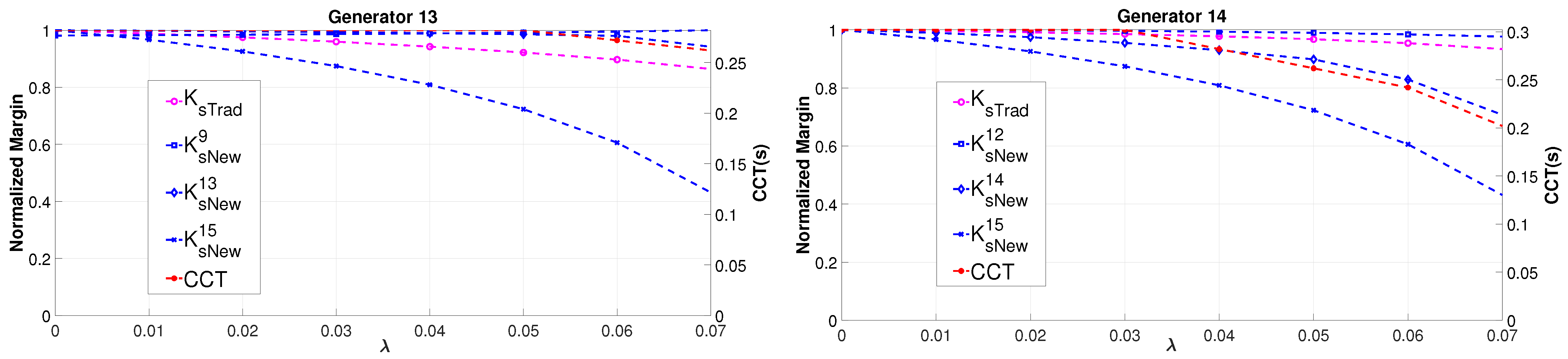
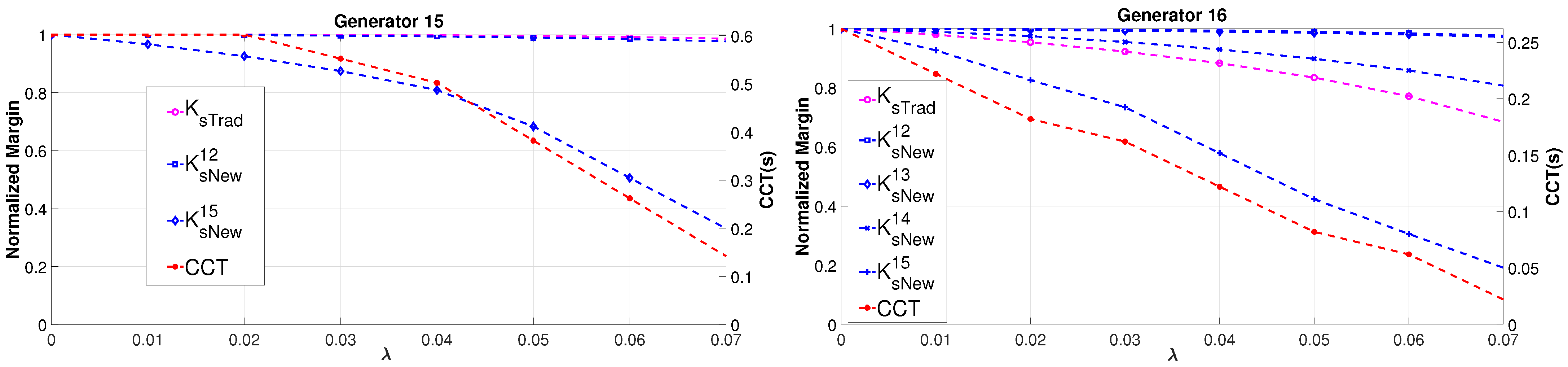
The CCT value analysis of the New England 68-bus test system simulation results, four generators $G_{13}$, $G_{14}$, $G_{15}$ and $G_{16}$ with decreasing CCT value over the range of $\lambda$ variations and are considered as the critical generators. Compared to other generators, the transient stability margin of the critical generators is the least, and becomes unstable quickly during disturbances. Therefore, the generators with the lowest CCT values are commonly considered as the critical generators. From Table 1, the critical generators’ associated electromechanical modes can be identified and the proposed stability index must be calculated only for these associated electromechanical modes.

Figure 4 plots the transient stability margin variations of the critical generators $G_{13}$, $G_{14}$, $G_{15}$ and $G_{16}$ over the range of 0 to 0.07 values of $\lambda$. The generators’ proposed transient stability margin values related to the electromechanical modes are determined separately and plotted under the same graph with the variables $K_{sNew}^9$, $K_{sNew}^{12}$, $K_{sNew}^{13}$, $K_{sNew}^{14}$ and $K_{sNew}^{15}$. Generators 15 and 16 show a sharp decline in CCT values, indicating more loss of transient stability margin among the critical generators. The CCT values of generator 13 are slightly decreased from 0.28 s to 0.26 s, and the corresponding $K_{sNew}^9$ values follow the same variations with the decrease to 0.94 of its normalized value. For generators 14, 15 and 16, the CCT values decreased from 0.30 s, 0.60 s, 0.26 s to 0.20 s, 0.14 s and 0.02 s, respectively. The corresponding $K_{sNew}^{14}$ and $K_{sNew}^{15}$ values of the generators decreased to 0.70, 0.33 and 0.19 of their normalized values, and follow the CCT curves. Therefore, the proposed transient stability margin corresponding to each electromechanical mode shows a more accurate transient stability margin based on the generators’ contributions to the corresponding electromechanical mode.

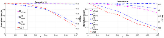
Figure 4. Transient stability analysis of critical generators in New England 68-bus test system.

5. Conclusions

This research proposed a new transient stability index for a multimachine interconnected power system based on synchronizing the torque contributions of all other connected generators. The proposed margin is verified with the most popular transient stability indicator, CCT, and compared with the generators’ traditionally determined synchronizing torque values. The proposed margin shows the system’s transient stability limit in terms of synchronizing torques for each generator separately, and is more accurate than the traditional stability indicator, which considers only individual generators’ synchronizing torques. Hence, the system operator can use this more accurate indication of the transient stability index for planning and operation studies, and take essential measures to improve the system’s stability through the concerned individual generators. The simulations are performed over a small WSCC 9-bus test system and a large New England 68-bus test system. For future work, the synchronizing torque contributions of all machines on the transient stability margin of renewable penetrated interconnected power systems must be accurately determined and verified.

References

- Haes Alhelou, H.; Hamedani-Golshan, M.E.; Njenda, T.C.; Siano, P. A survey on power system blackout and cascading events: Research motivations and challenges. Energies 2019, 12, 682. [Google Scholar] [CrossRef] [Green Version]
- Wu, Y.K.; Chang, S.M.; Hu, Y.L. Literature review of power system blackouts. Energy Procedia 2017, 141, 428–431. [Google Scholar] [CrossRef]
- Złotecka, D.; Sroka, K. The characteristics and main causes of power system failures basing on the analysis of previous blackouts in the world. In Proceedings of the 2018 International Interdisciplinary PhD Workshop (IIPhDW), Swinoujscie, Poland, 9–12 May 2018; pp. 257–262. [Google Scholar]
- Kundur, P.; Paserba, J.; Ajjarapu, V.; Andersson, G.; Bose, A.; Canizares, C.; Hatziargyriou, N.; Hill, D.; Stankovic, A.; Taylor, C.; et al. Definition and classification of power system stability IEEE/CIGRE joint task force on stability terms and definitions. IEEE Trans. Power Syst. 2004, 19, 1387–1401. [Google Scholar]
- Nagel, I.; Fabre, L.; Pastre, M.; ç ois Krummenacher, F.; Cherkaoui, R.; Kayal, M. High-speed power system transient stability simulation using highly dedicated hardware. IEEE Trans. Power Syst. 2013, 28, 4218–4227. [Google Scholar] [CrossRef]
- Fouad, A.A.; Vittal, V. Power System Transient Stability Analysis Using the Transient Energy Function Method; Prentice-Hall: Englewood Cliffs, NJ, USA, 1991. [Google Scholar]
- Xue, Y.; Van Cutsem, T.; Ribbens-Pavella, M. A simple direct method for fast transient stability assessment of large power systems. IEEE Trans. Power Syst. 1988, 3, 400–412. [Google Scholar] [CrossRef]
- Xue, Y.; Van Custem, T.; Ribbens-Pavella, M. Extended equal area criterion justifications, generalizations, applications. IEEE Trans. Power Syst. 1989, 4, 44–52. [Google Scholar] [CrossRef]
- Vu, T.L.; Turitsyn, K. Lyapunov functions family approach to transient stability assessment. IEEE Trans. Power Syst. 2015, 31, 1269–1277. [Google Scholar] [CrossRef] [Green Version]
- Wang, S.; Yu, J.; Zhang, W. Transient stability assessment using individual machine equal area criterion PART I: Unity principle. IEEE Access 2018, 6, 77065–77076. [Google Scholar] [CrossRef]
- Wang, S.; Yu, J.; Zhang, W. Transient stability assessment using individual machine equal area criterion part II: Stability margin. IEEE Access 2018, 6, 38693–38705. [Google Scholar] [CrossRef]
- Liu, C.; Sun, K.; Rather, Z.H.; Chen, Z.; Bak, C.L.; Thøgersen, P.; Lund, P. A systematic approach for dynamic security assessment and the corresponding preventive control scheme based on decision trees. IEEE Trans. Power Syst. 2013, 29, 717–730. [Google Scholar] [CrossRef]
- Yan, R.; Geng, G.; Jiang, Q.; Li, Y. Fast transient stability batch assessment using cascaded convolutional neural networks. IEEE Trans. Power Syst. 2019, 34, 2802–2813. [Google Scholar] [CrossRef]
- Kamwa, I.; Samantaray, S.; Joós, G. On the accuracy versus transparency trade-off of data-mining models for fast-response PMU-based catastrophe predictors. IEEE Trans. Smart Grid 2011, 3, 152–161. [Google Scholar] [CrossRef]
- Shaltout, A.; Al-Feilat, K.A. Damping and synchronizing torque computation in multimachine power systems. IEEE Trans. Power Syst. 1992, 7, 280–286. [Google Scholar] [CrossRef]
- Abu-Al-Feilat, E.; Bettayeb, M.; Al-Duwaish, H.; Abido, M.; Mantawy, A. A neural network-based approach for on-line dynamic stability assessment using synchronizing and damping torque coefficients. Electr. Power Syst. Res. 1996, 39, 103–110. [Google Scholar] [CrossRef]
- Kamari, N.A.M.; Musirin, I.; Othman, M.M. EP based optimization for estimating synchronizing and damping torque coefficients. Aust. J. Basic Appl. Sci. 2010, 4, 3741–3754. [Google Scholar]
- Mohamed Kamari, N.A.; Musirin, I.; Dagang, A.N.; Mohd Zaman, M.H. PSO-based oscillatory stability assessment by using the torque coefficients for SMIB. Energies 2020, 13, 1231. [Google Scholar] [CrossRef] [Green Version]
- Anderson, P.M.; Fouad, A.A. Power System Control and Stability; John Wiley & Sons: Hoboken, NJ, USA, 2008. [Google Scholar]
- Chow, J.H.; Sanchez-Gasca, J.J. Power System Modeling, Computation, and Control; John Wiley & Sons: Hoboken, NJ, USA, 2020. [Google Scholar]
- Vittal, V.; McCalley, J.D.; Anderson, P.M.; Fouad, A. Power System Control and Stability; John Wiley & Sons: Hoboken, NJ, USA, 2019. [Google Scholar]
- Bakhtvar, M.; Vittal, E.; Zheng, K.; Keane, A. Synchronizing torque impacts on rotor speed in power systems. IEEE Trans. Power Syst. 2016, 32, 1927–1935. [Google Scholar] [CrossRef] [Green Version]
- Sauer, P.W.; Pai, M.A.; Chow, J.H. Power System Dynamics and Stability: With Synchrophasor Measurement and Power System Toolbox; John Wiley & Sons: Hoboken, NJ, USA, 2017. [Google Scholar]
- Kundur, P. Power System Stability and Control; McGraw-Hill: New York, NY, USA, 1994. [Google Scholar]
- Mithulananthan, N.; Canizares, C.A.; Reeve, J.; Rogers, G.J. Comparison of PSS, SVC, and STATCOM controllers for damping power system oscillations. IEEE Trans. Power Syst. 2003, 18, 786–792. [Google Scholar] [CrossRef]
- Roberts, L.G.; Champneys, A.R.; Bell, K.R.; di Bernardo, M. Analytical approximations of critical clearing time for parametric analysis of power system transient stability. IEEE J. Emerg. Sel. Top. Circuits Syst. 2015, 5, 465–476. [Google Scholar] [CrossRef] [Green Version]
- Sharma, S.; Pushpak, S.; Chinde, V.; Dobson, I. Sensitivity of transient stability critical clearing time. IEEE Trans. Power Syst. 2018, 33, 6476–6486. [Google Scholar] [CrossRef] [Green Version]
- Wu, Y.K.; Lee, T.C.; Hsieh, T.Y.; Lin, W.M. Impact on critical clearing time after integrating large-scale wind power into Taiwan power system. Sustain. Energy Technol. Assess. 2016, 16, 128–136. [Google Scholar] [CrossRef]
- WSCC 9-Bus System—Illinois Center for a Smarter Electric Grid (ICSEG). Available online: https://icseg.iti.illinois.edu/wscc-9-bus-system/ (accessed on 3 May 2022).
- New England 68-Bus Test System—Illinois Center for a Smarter Electric Grid (ICSEG). Available online: https://icseg.iti.illinois.edu/new-england-68-bus-test-system/ (accessed on 3 May 2022).
- Milano, F. An open source power system analysis toolbox. IEEE Trans. Power Syst. 2005, 20, 1199–1206. [Google Scholar] [CrossRef]
- Cañizares, C.A.; Mithulananthan, N.; Milano, F.; Reeve, J. Linear performance indices to predict oscillatory stability problems in power systems. IEEE Trans. Power Syst. 2004, 19, 1104–1114. [Google Scholar] [CrossRef]
Publisher’s Note: MDPI stays neutral with regard to jurisdictional claims in published maps and institutional affiliations. |
© 2022 by the authors. Licensee MDPI, Basel, Switzerland. This article is an open access article distributed under the terms and conditions of the Creative Commons Attribution (CC BY) license (https://creativecommons.org/licenses/by/4.0/).