Abstract
This work presents a comparison of alternating current (AC) and direct current (DC) distribution systems for a residential building equipped with solar photovoltaic (PV) generation and battery storage. Using measured PV and load data from a residential building in Sweden, the study evaluated the annual losses, PV utilization, and energy savings of the two topologies. The analysis considered the load-dependent efficiency characteristics of power electronic converters (PECs) and battery storage to account for variations in operating conditions. The results show that DC distribution, coupled with PV generation and battery storage, offered significant loss savings due to lower conversion losses than the AC case. Assuming fixed efficiency for conversion gave a 34% yearly loss discrepancy compared with the case of implementing load-dependent losses. The results also highlight the effect on annual system losses of adding PV and battery storage of varying sizes. A yearly loss reduction of 15.8% was achieved with DC operation for the studied residential building when adding PV and battery storage. Additionally, the analysis of daily and seasonal variations in performance revealed under what circumstances DC could outperform AC and how the magnitude of the savings could vary with time.
1. Introduction
The solar photovoltaic (PV) and battery markets have seen rapid price reduction and exponential growth in recent years [1,2]. The interest in direct current (DC) systems has also gained more momentum following the latest technological development in power electronics [3] and the increased penetration of PV and battery storage [4]. As PV modules generate DC and batteries operate with DC, a DC topology enables efficient interaction between the two, with fewer power semiconductors in the current path for voltage conversion. Furthermore, almost all electronic loads in buildings are DC-operated [5]. Lastly, the expected growth in electric vehicles, which are also DC-operated, is an additional motivator for DC in and adjacent to buildings [6]. Today’s conventional alternating current (AC) topologies require conversions between AC and DC before the final user stage, generating losses. Adopting DC distribution reduces or even avoids some conversion losses, thereby increasing the system performance. In an expert survey among market stakeholders [7], the top priority identified for further DC market penetration was the need for more research on this topic.
Many attempts have been made to estimate the energy savings when switching from AC to DC distribution in buildings. The reported findings differ substantially, with reported savings of up to 25%, depending on the chosen reference case, types of appliances (i.e., loads included), and systems studied (with or without PV and battery) [8,9,10,11,12,13], including studies where no energy savings are observed [12]. In [8], the study’s novelty includes the use of real household profiles from 120 residential buildings, unlike previous studies where synthetic profiles are used [9,12,14,15]. Here, savings vary between 9 and 20% and increase to 14–25% with the inclusion of battery storage. Vossos et al. used synthetic load and PV profiles in 14 cities in the US to determine the energy savings derived from DC distribution [9]. The cities were chosen to examine the effect of varying solar radiation, and the findings report savings in the range of 5–14%. Siraj et al. compared the performance of a DC home at three DC voltage levels (48, 220, and 380 VDC) and a 220 VAC case and reported savings of 4–10% at the highest DC voltage levels [11]. Dastgeer et al. performed a comparative study of AC and DC distribution in a residential building and concluded that no energy savings were achieved with DC [12]. However, previous works [3,10,16,17,18] acknowledge that including PV and battery as native DC generator and storage, respectively, is a prerequisite for achieving energy savings with DC. These components were not included in [12]. A comprehensive simulation comparison for zero net energy (ZNE) office buildings by [17] shows a significant variation in savings, ranging between 1 and 18%. The variation comes from parametric simulations varying PV, battery, and power electronic converter (PEC) sizes and demonstrates the effect of the system design on energy savings. Ahmad et al. performed a day-by-day comparative analysis of AC and DC distribution performance in a residential building and analysed the output through parametric simulations of PEC efficiency, solar power, and seasonal variation [18]. The work by Alshammari et al. reports a 5% reduction in annual grid energy with DC distribution in a commercial building (school) [19]. This study also compares the seasonal variations in energy savings by studying days of the four seasons. Spiliotis et al. studied the energy savings in an office building in five geographical locations; they concluded that 380 VDC outperformed the conventional 230 VAC in terms of energy efficiency and presented a loss split for the included components [20]. To minimise the conversion losses for AC and DC operation, [21] demonstrated a system control scheme for the internal power flows and source origin (grid, PV, or battery). Chinnathambi et al. performed measurements at the sources in this real-life demonstration, but it remains unclear how the control scheme treats the converter losses.
As pointed out in previous works, e.g., [16,17,22], this research topic requires more comprehensive efforts, deepening the detail level of modelling to enable an accurate comparison of the two topologies. A comprehensive review article by Gelani et al. [23] concludes that the findings from previous works are conflicting, and the combined efforts fail to give a final verdict on the feasibility of DC operation and under what circumstances DC is favourable. Table A1 gives an overview of related journal publications on DC energy savings in buildings concerning methods, data profiles, and inclusion of DC sources, i.e., solar photovoltaic (PV) and battery. The last row in the table relates this work to previous efforts.
Typical in previous works, e.g., [9,11,14,24], is the use of constant efficiency for power electronic converters (PECs) and battery when assessing the energy savings derived from DC distribution. This approach neglects the load-dependent efficiency characteristics, which represent a deciding factor for an accurate comparison [10,17,18,20,23,25]. Despite acknowledging the importance of load-dependent efficiency, [12] only includes a variety of fixed efficiency values when quantifying the effect of the converter characteristic. Studies acknowledging the efficiency load dependency are, e.g., [15,17,20]. However, the presented PEC efficiency curves only include part of the loading range and thus make it unclear how the low loading range is treated in modelling. Using constant efficiency or neglecting the entire operating range—without considering PEC power operating constraints in the latter case—leads to inaccurate results. Examples of varying efficiency characteristics and their effect on system performance are examined in [12,18,26]. However, these studies only present the effect on a single day’s performance [18,26] or the effect of various constant efficiency values [12]. While the referred studies leave room for improvement, they demonstrate the need for the proper modelling of converters for a fair and accurate comparison.
In addition to constant efficiency, another gap is the access and usage of data profiles (PV and load) in modelling [23]. Several of the previous studies use synthetic profiles for the full-year comparison, and these are either based on average profiles [9,12,17,18] or modelled using building and occupant-specific factors [20,27]. Averaging data leaves out peaks and variations while modelling synthetic data using performance indexes, e.g., internal heat dissipation (W/person or appliance) and ventilation flow rates (l/s), often resulting in repetitive profiles that may not reflect the building actual behaviour. Another vital aspect for an accurate comparison is the data period analysed, where comparisons based on a single day’s operation [15,18,21] neglect the seasonal variations in load and PV profiles. Ref. [15] presents daily variation in energy savings with DC operation, but as proven in other studies, seasonal variations also affect the performance [18,19,27,28]. With these arguments, an accurate comparison requires full-year, measured operation data of both PV and load profiles.
Furthermore, other studies identify the need for more detailed modelling of the battery losses and dynamic load behaviour [17,23], which previous important works [8,9,17] lack.
Given the identified gaps, the topic needs more detailed analyses to address whether a DC topology results in lower losses, and if so, to what extent, and the decisive factors. The latter is also identified as a top priority in an expert assessment on the future of direct current in buildings [22]. This work aims to evaluate and quantify the performance of AC and DC distribution in a residential building. The work addresses the gaps identified above by including measured efficiency characteristics of PECs and battery and evaluating the performance using a full-year data set of load usage and PV generation. The results include the relative effect of including DC sources (PV and battery) and challenge the assumption of using constant PEC efficiency. Furthermore, an examination of the daily and seasonal performance of the two topologies statistically determines when DC is a favourable option for loss reduction in the studied case. This study completes previous efforts and contributes to the current field with the following:
- Experimentally obtained efficiency characteristics of power electronic converters (PECs) and battery cells;
- Quantification of the loss discrepancy when using fixed and load-dependent converter and battery efficiencies;
- Quantification of the effect on the system technical performance of the inclusion of a PV and battery system;
- The magnitude of the loss origins in the AC and DC topologies;
- Statistical identification of most significant correlating factor for DC savings.
The remainder of the work is outlined as follows: Section 2 introduces the theoretical framework, and Section 3 presents the case setup, including the residential building and modelled topologies. Section 4 describes the PEC measurements and resulting efficiency characteristics, and Section 5 presents the modelling approach and evaluation metrics. In Section 6, the results are presented and discussed, and concluding remarks are presented in Section 7.
2. Theory
2.1. AC Building Topology with PV and Battery System
In urban areas with access to a shared electrical grid, AC power is the primary source of electricity in buildings. Figure 1 illustrates a typical AC configuration for a residential building with solar PV and battery storage. In this system, loads are divided into “big” and “small” based on the maximum power, and it is assumed that these needs are met using DC power in the final stage.
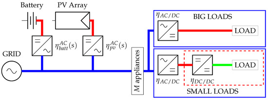
Figure 1.
Modelled AC distribution topology with AC-coupled PV and battery system.
The small loads require two conversion steps [12]: firstly rectification (AC/DC) and then DC/DC conversion, where the needed galvanic isolation in the distribution is realized in the later stage. A power flow path from PV energy, p, to the load through intermediate battery storing reveals that several conversion steps are needed to meet the load demand, p, as seen in Figure 1.
where the PV array and the battery storage AC/DC efficiency values, (s) and (s), respectively, are functions of loading (s); and and are load-specific conversions.
In Figure 1, the PV and battery are connected through the main AC link (AC-coupled). An alternative method, in which the PV or battery is connected to the primary DC link, is outlined in [29]. Here, it is important to point out that this configuration brings some impracticality, such as a varying DC voltage level. The DC coupling complicates the charge control of the battery and adds costs for the other conversion units, since they have to be designed for a substantially varying voltage level. Accordingly, this solution is omitted in further investigations in this article.
2.2. Electrical Losses in Buildings
Losses in an electrical system occur in the cable power transfer (conduction) and through conversions between voltage levels and between different states, i.e., inversion (DC/AC) or rectification (AC/DC). The relation among power, current, and voltage is
where p(t) is the power, u(t) is the branch voltage, and i(t) is the current.
2.2.1. Cable Conduction Losses
For a power demand , the conduction losses, , in the cable can be expressed using the following relation:
where is the load current and R is the cable resistance. For a DC topology, u(t) and i(t) are equal to u(t) and i(t). For the AC topology, cos() = 1 is assumed, and u(t) and i(t) are equal to u and i, respectively. In addition, harmonics are neglected, which, together with the cos() assumption, underestimates the losses for the AC system. The cable resistance, R, in (3) is given as
where is the resistivity of the cable material, L is the length of the cable, and A is the cable cross-section area [10]. The minimum cable area is chosen with consideration of the thermal limitations. The necessary cable cross-section area for a building is found in the IEC 60228 standard [30], as shown in Table 1. The table also specifies the cable resistance per meter length, using (4).

Table 1.
Standardised cable cross-section area per maximum current according to IEC 60228 and the corresponding resistance per meter from (4), using the resistivity of copper (0.0171 mm/m).
2.2.2. Voltage Conversion Losses
Few loads operate directly on the incoming 230/110 AC voltage, and conversion between voltage levels, and AC and DC is performed in different ways. When supplying the smaller loads, a so-called power factor correction (PFC) circuit is typically used that consists of a diode bridge rectifier followed by a boost converter step. The large-load AC/DC rectifiers can either be a PFC circuit or a three-phase transistor rectifier, and in this work, the bidirectional AC/DC converters are assumed to consist of transistor bridges. The conversion efficiency is calculated using the ratio of input and output powers as
where the inputs and outputs can be either AC or DC at different voltage levels. The corresponding conversion losses are then calculated as
where p(t) is the converter power throughput, including load demand and converter losses.
3. Case Setup
A comparison of AC and DC operations was made for a residential building located in Sweden, with space and domestic hot water heating generation using a ground-source heat pump. The house was developed and built within a EU-FP7 collaborative project (Need4b—http://need4b.eu/?lang=en, URL accessed 18 January 2023) to demonstrate cost-effective and energy-efficient technologies. Fourteen PV panels (each of 260 kWp) were installed at a 45 tilt angle due south to help to achieve the primary energy consumption target of 60 kWh/m/a. Blueprints and more detailed information about the house can be found in [10].
3.1. Electrical Load and Photovoltaic Profiles
Measured data of the load and PV generation with temporal resolution of 15 min were used as the basis for this study. Figure 2 shows the daily load demand and PV generation, which display a clear seasonal miss-correlation.
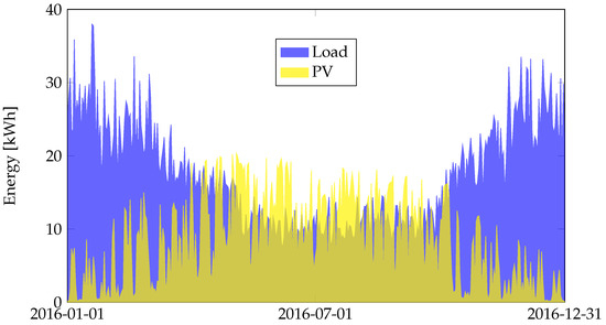
Figure 2.
Daily load demand and PV generation of the residential building.
Individual measurements were obtained for the following appliances: ground-source heat pump, ventilation, water pumps, and PV generation. As there were no individual measurements of the other appliances, synthetic profiles for lighting and other appliances were created and used with the measured profiles. The works in [31,32] were used as inspiration for the load profiles of the white goods. A comparison was made with the measured aggregated profile to verify the magnitude and time distribution to verify the synthetic profiles. The annual load demand for the studied year was 6354 kWh, and the PV-generated energy was 3113 kWh, both in AC quantities.
3.2. Proposed DC System Topology with PV and Battery System
Figure 3 shows an example of a DC topology for a residential house with two DC voltage levels for larger (“big”) and smaller (“small”) loads (the loads are distinguished as “big” and “small” depending on their rated power). The larger loads were operated directly via the main DC bus, and the smaller loads were fed via a DC/DC converter. The studied typology determined the distribution voltage, i.e., 230 VAC or 380/20 VDC for AC or DC, respectively. This study was performed for a grid-tied building; a bidirectional AC/DC converter was needed for grid interaction.
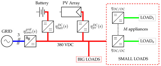
Figure 3.
Modelled DC distribution topology with individual converters for the PV and battery system. Loads are distinguished as ”BIG” and ”SMALL” depending on their rated powers, where the m smaller loads are supplied by 20 VDC via galvanically isolated DC/DC converters.
The DC topology allowed the energy generated by the PV system to be more efficiently used than the AC topology, as shown in Figure 1, because DC/DC conversion was more efficient than the AC/DC equivalent. Using the same power flow example as in (1), the equivalent conversion steps could be reduced from five to four.
where the low-power DC/DC conversion () is equal for both the AC and DC topologies, as indicated by the dashed perimeters in Figure 1 and Figure 3.
3.3. Investigated System Topologies
In this study, four system topologies were modelled and compared with regards to their technical performance:
- AC—230 VAC with load-dependent efficiency.Conventional system. See Figure 1 for the system layout including PV and battery system. Here, cable conduction losses occurred with the 230 VAC distribution.
- DC—380 VDC with load-dependent efficiency.Conduction losses with 380 VDC distribution. This voltage level was chosen from the EMerge Alliance 380 VDC standard for data centre power distribution [33,34,35] and the result of an expert assessment [22] of suitable DC distribution levels.
- DC—380 VDC with fixed converter efficiency.To quantify the loss discrepancy with DC, fixed efficiency values were used for all converters and the battery. This represented the approach used in previous works [12,14,36].
- DC—380 and 20 VDC with load-dependent efficiency.A 20 VDC sub-voltage level was added to DC and DC to supply the smaller loads and lighting through a central DC/DC converter (see Figure 1 in [37] for an example of such a system topology). Since this "Class A" voltage level is considered not to be dangerous for humans, safety designs are substantially cheaper [38]. Additionally, this sub-voltage level aligns with the supply voltage of the USB Type–C standard.
4. Power Electronic Converter Measurements
Due to the variation in converter performance discrepancies found in the literature [9,24,39,40,41,42] and to model the efficiency characteristics, laboratory measurements were made on three power electronic converters (PECs). These included: (i) a 14 kVA transformerless bidirectional converter with a neutral-point-clamped (NPC) topology, (ii) a 6 kW transformerless bidirectional (DC/DC) buck–boost converter with two interleaved legs, and (iii) a 6 kW transformerless unidirectional boost (DC/DC) converter with two interleaved legs. In Figure 3, the bidirectional converter is located between the AC grid and the DC main link voltage; the bidirectional DC/DC converter, at the battery; and the unidirectional DC/DC converter, at the PV array.
4.1. Experimental Setup
Measurements were made in the complete operating range of the converters, and the efficiency characteristics were calculated using (2) and (5). For the bidirectional converters, measurements were taken in both directions. A Norma D6100A watt meter was used to measure the current and voltage of the DC/DC solar converter and the AC side of the bidirectional AC/DC converter, while data of the DC side of the bidirectional converter were acquired using Yokogawa WT1600. The total power measurement uncertainty was 0.2%. In Figure 4, the measurement setup is shown for the 14 kW bidirectional AC/DC converter.
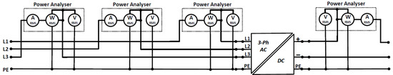
Figure 4.
Measurement setup for the bidirectional AC/DC converter.
4.2. Results—Converter Measurements
Figure 5 shows the measurement points and curve fit for the three converters.
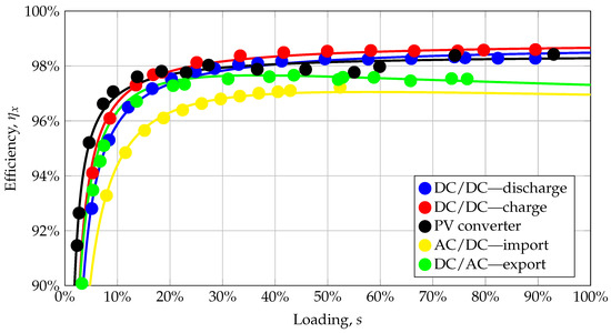
Figure 5.
Resulting converter efficiency values and curve fit derived from measurements.
Curve fitting was performed using a rational polynomial as
where p(s) is the ratio of the converter loading to its rated power. The numerical values of k and m in (8) can be found in Table A2 for the respective converters. The bidirectional DC/DC converter was measured for charge and discharge. The resulting difference was due to the converter topology, where the latter was performed using the buck combination semiconductors and the former was performed through the boost combination of the semiconductors. The results show that the assumption of fixed efficiency might be sufficient under loading >20% but greatly overestimates the performance for points below that.
5. System Modelling
System modelling was based on a power flow analysis using the PV generation and load usage time-series profiles from Section 3.1 with 15-minute temporal resolution. The measured PV data are in AC quantity, and the gross yield generated by the PV array, that is, before MPPT and inverter, was calculated as
where (s) is the inverter efficiency as a function of loading.
The battery control operated to minimize the grid interaction, as it has been identified in related studies that grid interaction disfavours the DC topology [10,20]. Figure 6 describes the battery charge and discharge conditions, where SOC(t) is the battery state of charge (SOC) in each time step and (s) is the total efficiency of battery conversion, including losses of the battery cell [10] and the converter for topology j (AC ∨ DC).
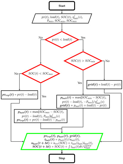
Figure 6.
Flow chart of battery charge and discharge control.
Here, the battery voltage level, u(t), is adjusted for the next time step using the current and internal resistance, r(i), and the battery open-circuit voltage (OCV) as functions of its SOC, all adopted from previous work of the author [10]. Lastly, the battery SOC level, SOC(t + t), is adjusted for the next time step. The battery operating SOC range was set to 15–90% (SOC and SOC, respectively), and the variation in internal battery resistance was set as a function of the current adopted from [10].
The case study was for a PV/battery system of 3.68 kWp and 7.5 kWh, respectively, and a charge/discharge limitation, P, of 6 kW. The selected battery size was derived from a related study in [43], which concluded that for the studied user case, limited additional gains in self-consumption were seen for battery sizes exceeding 7.5 kWh.
5.1. Loss Modelling
The following sections describe the conduction- and conversion-loss modelling methodology and introduce the evaluation performance metrics.
5.1.1. Cable Conduction Losses
For the modelling of the conduction losses, the feeder lengths defined based on the house drawings (see Appendix A in [10]) were used together with the distribution voltage, U, and (3) and (4). The cable cross-section area from Table 1 was fixed for each appliance and set according to the maximum current of one year’s operation in each cable branch. For the lighting, it was assumed that the current to each room, being the sum of the current to all active lamps, was fed through one cable and then distributed to individual branches depending on the lighting layout [10]. Each room consisted of 2–11 LED lights at 7 W each. The model treated individual room sockets similarly by distributing common current to the active socket(s) at each time step. In addition, stationary appliances has a fixed feeder length, and conduction losses were calculated using (3) and (4).
5.1.2. Converter Losses
Both the AC and DC topologies were operated with fixed main link voltage levels (230 VAC and 380 VDC, respectively). Therefore, the battery voltage had to be converted to the desired voltage using a converter, and these losses were calculated as
where (s) is the load-dependent efficiency for topology j and p(t) is the battery power. In addition to the losses of the battery converter, the losses of the battery cell—caused by the internal resistance—were included and modelled with varying resistance as a function of the current, r(i), as [10]
where the relation between battery cell resistance and current, r(i), was taken from [10].
The losses of the PV converter (PV inverter for the AC topology) were calculated using the gross yield, p(t), from (9) as
where the efficiency characteristics, (p), are dependent on the modelled topology, j.
A summary of the efficiency characteristics used in the modelling is given in Table 2 for the four cases (AC, DC–DC).
Table 2.
Efficiency characteristics used for system modelling in each of the four cases.
Here, f(s) denotes efficiency varying with converter loading (s), and and are the load-side conversion efficiency values (see Figure 1 and Figure 3). The last DC/DC conversion for the low-power appliances, , was present in both topologies and did not affect the relative comparison since they were treated equally. The losses of the grid-tied bidirectional converter were calculated using both load-dependent (DC) and fixed (DC) efficiency characteristics, as explained in Section 3.3. The fixed efficiency was set to 97.6% to match the peak efficiency of the AC/DC converter from the measurements. The converter was modelled with a rated power to match the annual load peak, 6.2 kW, to always enable load coverage. The efficiency characteristics of the PV and battery converters in the AC case were extracted from the measurements in Section 4.2 with a −1.5-percentage-point offset from the efficiency curve caused by extra-semiconductor crossing [10]. In the AC topology, AC/DC conversions were performed with an H-bridge for each load, and the operation was binary (ON/OFF), with fixed efficiency of 97% [10]. In DC, the peak efficiency values from the measurements were used for the grid, battery, and PV converters.
5.2. Building Performance Metrics
In addition to loss savings, the topologies were evaluated for their PV utilisation factor, , which defines the useful PV energy, with the losses of the PV converter (PV inverter for the AC topology) and battery storage (including battery cell losses) being taken into consideration. When battery charging is solely performed via PV surplus, PV utilisation is defined, in [27], as
where p are the losses of the battery converter; p are the battery cell losses; p are the losses of the PV converter, calculated with (10)–(12), respectively; and p is the generated gross PV energy calculated with (9). The numerator denotes the PV-associated losses. Another metric, defined in [17] as the system efficiency, relates the annual losses to the total load demand as
where E is the annual load demand, which is equal for all modelled topologies and cases. The total loss, E, for topology j was calculated using (3), (6), and (10)–(12) as
where p(t) is the sum of all M load-side converter losses, and in the DC topology, these also include the grid-tied bidirectional converter.
6. Results and Discussion
This work quantified the loss savings of a DC topology and the resulting discrepancy when using load-dependent and fixed efficiencies. The analysis used the measured load and PV profiles presented in Section 3.1 on the topologies in Section 3.3. Section 5 outlines the system modelling and includes the PEC measurement results in Section 4.2.
The annual losses of the four topologies (Figure 7) without PV and battery storage resulted in three observations:
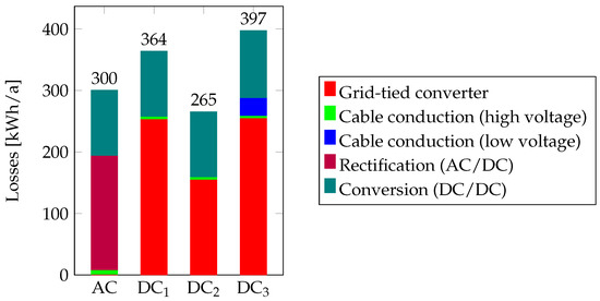
Figure 7.
Annual system losses in the four modelled cases without PV and battery storage.
- The bidirectional converter losses significantly differed when modelled with fixed and load-dependent efficiency characteristics; see cases DC and DC. Assuming constant efficiency as in many previous studies, e.g., [39,44,45], was thus not eligible. As this study was for a residential building with varying net grid interaction, the converter covered the entire load range during operation. Considering the efficiency characteristics of the converter (see Figure 5), the constant efficiency approach was relatively accurate under loading >20% but underestimated the losses below that loading. The results also suggest that with assumed constant efficiency, the DC topology could achieve energy savings even without the inclusion of PV or battery storage, contradicting the findings in [8,9,17]. In relative numbers, the losses of the grid-tied converter using a constant efficiency approach (DC) were 34% lower (or in absolute terms, an underestimation of 63 kWh) than those in the case implementing load-dependent efficiency (DC). Using (14), the system efficiency values of the respective systems (AC and DC) were 95.3, 94.3, 95.8, and 93.7%, respectively.
- Adding a DC sub-voltage level (DC) added 7.3% (29.0 kWh/a) to the total losses when operated at 20 VDC. These added losses also transferred to the load-side conversion (DC/DC) losses, which were 3% higher with DC than in the other cases. The cable conduction losses, identified in [23] as an essential factor to consider, amounted to 2.4 and 1.5% of the total losses in the AC and DC cases, respectively, which is in line with findings in previous works [46,47].
- Without the inclusion of PV and battery, the DC topology did not present a favourable option in terms of loss reduction (excluding case DC with the reasoning performed in 1). This result confirms the findings in previous works [8,9,17,22,24].
Based on these observations, the continuing analysis only includes the AC reference case and the DC topology with load-dependent converter efficiency (DC).
The comparison presented in Table 3 is for a system with a 3.7 kWp PV array and 7.5 kWh battery storage.
Table 3.
Comparison of system performance with AC and DC with 3.7 kWp PV and 7.5 kWh battery storage.
The generated PV energy was higher in the DC case, since it was fed directly to the DC link, with reduced conversion losses. With the inclusion of the DC sources (PV and battery storage), operation with the DC topology reduced the total annual losses by 15.8%. Figure 8 shows a loss breakdown per source in the two cases.
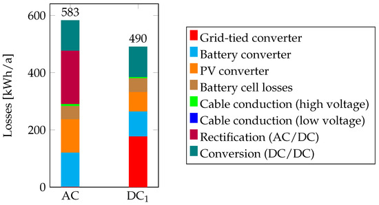
Figure 8.
Annual system losses for a system configuration with 3.7 kWp PV array and 7.5 kWh battery storage. Low-voltage cable conduction was zero for both topologies but is included in the legend for consistency with the other figures.
The effect of adding the DC sources is confirmed in [10,12,20]. The lowered losses through the bidirectional converter were due to the reduced grid interaction (see comparison with DC in Figure 7) when energy was generated and stored locally. Comparing the rectification losses in AC operation with the grid-tied converter in the DC case—having the same purpose (in addition to grid import rectification (AC/DC), the bidirectional grid-tied converter also inverts the grid export (DC/AC))—showed a 5.3% relative annual loss reduction with DC operation. The losses of the PV array and battery were lower in the DC case due to more efficient conversion (−41.4% and −27.3%, respectively), which affected the PV utilisation factor, , as shown in Table 3. In this case, the PV-associated losses of the PV converter, battery converter, and battery cells were 28.6% lower with the DC topology, resulting in a PV utilisation gain of 2.6% using (13). The system efficiency values from (14) were then 90.8 and 92.3% with the AC and DC topologies, respectively, thus resulting in a relative efficiency gain of 1.7%.
Figure 9 shows the power flow duration in annual operation as a function of respective converter loading. In Figure 9a, the grid-interaction is shown for import and export, which highlight the necessity to account for the load-dependent efficiency characteristics when modelling the losses.
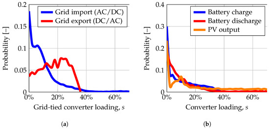
Figure 9.
Power flow distribution in annual operation for (a) grid import and export, and (b) battery charge and discharge, and PV generation.
Fixed efficiency, thus, underestimated the accumulated losses by ignoring frequent operation under low loading (with poor efficiency; see Figure 5). Similarly, Figure 9b shows the duration of battery charge, battery discharge, and PV output. Again, the majority of occasions occurred under low converter loading, which further stresses the importance of adopting the complete PEC efficiency characteristics.
To determine under what circumstances DC is a favourable option for loss reductions, Figure 10a shows a heat map of the loss difference in AC and DC operations sorted by daily hour (1–24) and month (1–12), where positive values indicate loss savings with DC operation.
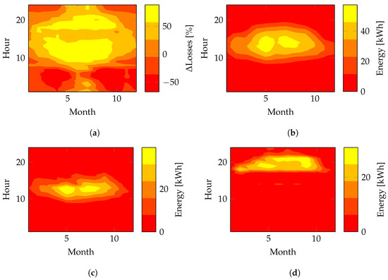
Figure 10.
Heat map per daily hour and month in 2016 showing (a) loss differences in AC and DC operations (positive values indicate savings with DC), (b) accumulated PV generation, and (c,d) accumulated battery charge and discharge, respectively.
When PV was present, DC operation resulted in lower losses, which correlates well with the results in Figure 10b. In the presence of battery storage and with the battery control described in Figure 6, the loss savings expanded to later in the day, when excess PV generation charged the battery (Figure 10c) and discharged to cover load surplus (see Figure 10d). Using Spearman’s rank coefficient of correlation [48], the loss savings showed the highest correlation (0.59) with PV generation. The loss saving dependency on available PV generation is also confirmed in previous works [27,49,50].
Figure 11 shows an expanded analysis of AC and DC by varying the sizes of the PV array and battery storage.
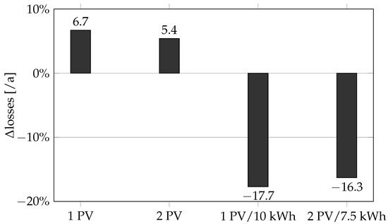
Figure 11.
Relative changes in annual losses during DC operation with various PV and battery system configurations. The -comparison is with reference to AC performance; thus, positive values indicate higher losses during DC operation.
Compared with the case without PV and battery in Figure 7, the inclusion of PV (“1 PV”) reduced the annual loss difference from +22% to +6.7% but was not sufficient for the DC case to achieve annual energy savings comparable to those with AC. A doubling of the PV array (“2 PV”) resulted in a marginal improvement in the relative comparison with the AC topology (+5.3%/a). Doubling PV also added +18.3% to the grid-tied converter losses due to increased PV export (see Figure 12).
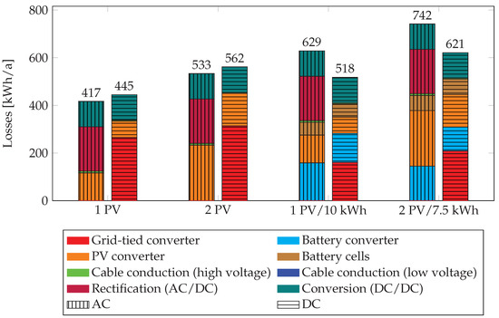
Figure 12.
Loss split in AC and DC operations and the modelled PV and battery system configurations. Low-voltage cable conduction is zero for all topologies but is included in the legend for consistency with the other figures.
The DC topology first achieved savings when including battery storage (“1 PV/10 kWh” and “2 PV/7.5 kWh”), as it reduced the interaction with the grid and thus the influence of the grid-tied converter. This reduction was due to the chosen battery control with the objective function to minimise the grid interaction, as presented in Section 5. The annual loss reductions with a battery included ("1 PV/10 kWh" and "2 PV/7.5 kWh" in Figure 11) were marginally greater than those in the case in Table 3. This trade-off between PV array and battery size, and annual savings is further investigated in [27], where it is concluded that the sizing of the PV array and the battery, for DC savings analysis, is important to avoid sub-optimisation.
This work, as well as several others, e.g., [10,17,20], quantified the effect of the grid-tied converter on the system performance and highlighted it as a critical component of the DC topology. Measures to reduce this impact include parallel converter operation, as suggested in [10,25], and demand-side management of suitable loads. Two parallel converters, with one being designed for high-efficiency operation at low power, can boost the grid-tied converter performance. In addition, shifting loads and avoiding these low-power operations can further reduce losses. Furthermore, as proven in previous works [27,49,50], the load and PV coincidence are decisive factors in DC operation loss savings. Awad et al. [51] present a method to design the PV array (in terms of orientation(s) and tilt angle(s)) to match the load demand and suggest to include this in future works.
7. Conclusions
This work compared the performance of a residential building with AC and DC distribution using measured performance characteristics of power electronic converters (PECs) and battery storage. The results used load and PV profiles measured during one year’s operation. The analysis included quantifying the DC loss savings when adding solar photovoltaic (PV) and battery storage and varying their respective sizes. The results present a quantitative comparison of the DC annual loss discrepancy when using fixed and load-dependent efficiency characteristics of the PECs. Three DC topologies were studied and compared to AC distribution: 380 VDC with load-dependent PEC efficiency (DC), 380 VDC with fixed PEC efficiency (DC), and DC with an added sub-voltage level (DC).
Comparing DC and DC, which had identical topologies, revealed a significant loss discrepancy when using fixed and load-dependent efficiencies. In this study, the loss discrepancy was 34% in a case without PV and battery storage. Analysing the converter loading showed that most interactions occurred in the low-load region with poor efficiency, thus highlighting the importance of using load-dependent efficiency. Therefore, load-dependent efficiency is essential when modelling realistic scenarios with a wide operating range.
The results show that with load-dependent PEC efficiency, internal conduction and conversion losses were reduced by 15.8% when switching from AC to DC, with PV and battery included. Furthermore, the DC topology increased PV utilisation by 2.6% with a 28.6% reduction in PV-associated losses. The analysis of hourly and seasonal variations in DC savings showed that Spearman’s rank coefficient showed the highest correlation (0.59) between DC savings and available PV generation.
The extended analysis showed that more than only adding PV was needed to achieve savings in the DC case compared with the AC case. The DC topology marginally improved when doubling the PV size, from +6.7% to +5.4% annual loss increase. However, when adding a battery, DC operation achieved substantial savings (up to 17.7% reduction), as the effect of grid-tied converter operation was reduced. The battery objective function to minimise the grid interaction due to export and import is a prerequisite for grid reduction and DC loss savings.
Above all, the results from this work show the relevance of modelling the conversion efficiency characteristics with load dependence to account for the PEC efficiency characteristics. Using the assumption of constant efficiency has proven inaccurate in the studied case with frequent converter operations in the lower power ranges and, thus, high relative losses. The presented efficiency characteristics of the converters and battery offer an accurate way to assess the potential for DC distribution in future studies.
Author Contributions
Conceptualization, P.O. and T.T.; Data curation, P.O.; Formal analysis, P.O.; Funding acquisition, P.O., T.T. and C.M.; Investigation, P.O. and T.T.; Methodology, P.O. and T.T.; Project administration, P.O.; Software, P.O.; Supervision, T.T., M.P. and C.M.; Visualization, P.O.; Writing—original draft, P.O.; Writing—review and editing, P.O., T.T., M.P. and C.M. All authors have read and agreed to the published version of the manuscript.
Funding
The Swedish Energy Agency funded this research through the national project “From photovoltaic generation to end-users with minimum losses—a full-scale demonstration” (2018–2020, grant number 43276–1) and the national project “Flexibility and energy efficiency in buildings with PV and EV charging” (2020–2023, grant number 50986–1).
Data Availability Statement
Not applicable.
Acknowledgments
The authors would like to thank Ferroamp for valuable discussions in conjunction with the measurement campaign.
Conflicts of Interest
The authors declare no conflict of interest.
Nomenclature
| A | Cable cross-section area |
| AC | Alternating current |
| DC | Direct current |
| Annual load demand | |
| Annual losses for topology j | |
| Energy imported from the grid | |
| j | Topology denotation (AC ∨ DC) |
| Rational polynomial curve-fitted constant () | |
| L | Cable length |
| Rational polynomial curve-fitted constant () | |
| NPC | Neutral-point-clamped |
| Power demand from load | |
| Power losses of component “x” | |
| Power to/from source “x” | |
| Gross energy yield from PV modules | |
| Maximum battery (converter) power | |
| PEC | Power Electronic Converter |
| pp | Percentage points |
| PV | Photovoltaic |
| PV energy exported to the grid | |
| Rated battery capacity (Ah) | |
| R | Resistance (in the cable) |
| Internal battery cell resistance | |
| SOC | Battery state of charge |
| SOC | Minimum battery state of charge |
| SOC | Maximum battery state of charge |
| Distribution voltage level | |
| Battery open-circuit voltage | |
| Combined battery efficiency, including converter and battery cell losses | |
| Efficiency of bidirectional grid-tied converter | |
| Efficiency of component “x” | |
| PV utilisation (subscript “PV”) or system efficiency (subscript “system”) | |
| Resistivity in cable material |
Appendix A
Table A1.
Taxonomy table of journal publications on AC vs. DC in buildings; methods, data profiles, DC sources included, data period analysed, and presented energy savings.
Table A1.
Taxonomy table of journal publications on AC vs. DC in buildings; methods, data profiles, DC sources included, data period analysed, and presented energy savings.
| PEC Efficiency | Data Profile | Battery Loss | DC Source | Data Period | Savings * | |||||||
|---|---|---|---|---|---|---|---|---|---|---|---|---|
| Ref. | Building Type | Load-Dependent | Fixed | Synthetic | Measured | Load-Dependent | Fixed | PV | Battery | Single Day(s) | Full Year | % |
| [8] | Residential | (✓) a | ✓ | ✓ | ✓ | ✓ | ✓ | 9–20 b | ||||
| [9] | Residential | ✓c | ✓ | ✓ | ✓ | ✓ | ✓ | 5 d | ||||
| [11] | Residential | ✓ | ✓ | – | – | ✓ | ✓e | 4–10% f | ||||
| [12] | Residential | ✓ | ✓ | – | – | ✓e | −6–−2% | |||||
| [15] | Residential | (✓) g | ✓ | ✓g | ✓ | ✓ | ✓ | – h | ||||
| [17] | Commercial | (✓) g | ✓ | ✓ | ✓ | ✓ | ✓ | 1–18% i | ||||
| [18] | Residential | ✓ | ✓ | – | – | ✓ | ✓ | – h | ||||
| [19] | Commercial | ✓ | ✓ | ✓ | ✓ | ✓ | ✓ | 5% | ||||
| [20] | Commercial | (✓) j | ✓ | ✓ | ✓ | ✓ | ✓ | 2–5% | ||||
| [21] | Residential | (✓) k | ✓ | – | – | ✓ | ✓ | – h | ||||
| [27] | Residential | ✓ | ✓ | ✓ | ✓ | ✓ | ✓ | 1–9% l | ||||
| This work | Residential | ✓ | ✓ | ✓ | ✓ | ✓ | ✓ | Section 6 | ||||
* Savings are either reported as energy savings in [8,9,19] or as system efficiency savings [11,12,15,17,18,20,27]. For a definition of system efficiency, see [17]. a Presents max and min values for the converters and claims that the same efficiency degradation is used for AC/DC and DC/DC PECs, but it is not clear whether the full efficiency range is considered in the loss analysis. b The savings increase to 14–25% when including battery storage. c Acknowledges the efficiency degradation at part load but only considers a single efficiency point below 20% of full-load operation. The work also includes a sensitivity analysis on PEC efficiency and concludes that improvements favouring either AC or DC will most likely concur; thus, the relative gains remain unchanged. d The savings increase to 14% when including battery storage. e Not explicitly mentioned, but to the best of our knowledge, it seems that the analysis is performed for an entire year’s operation. f The savings vary depending on the chosen DC distribution voltage (48–380 VDC) and wire gauge. g Presents efficiency curves for the PECs but only down to 10% part load. It is thus unclear how efficiency is treated in loading cases below 10%. h Only compares on the basis of a single day’s operation and thus not relevant to present savings in relation to the other studies. i The span represents the result from parametric simulations with varying PV and battery sizes for small and medium zero net energy office buildings. j Presents PEC efficiency curves down to 20% part load operation, but it is unclear how the efficiency is treated below that loading. k It remains unclear how the converter losses are treated. l Energy savings vary with the size of the PV/battery system and the geographical location studied.
Table A2 presents the numerical values for (8) to represent the converter efficiency characteristics. Figure 5 visualises the results as a function of converter loading.
Table A2.
Numerical values for the modelled converters to be used in (8).
Table A2.
Numerical values for the modelled converters to be used in (8).
| DC/DC | DC/DC | PV | AC/DC | DC/AC | |
|---|---|---|---|---|---|
| 0.9887 | 0.9876 | 0.9843 | 0.9617 | 0.9621 | |
| 0.607 | 0.662 | ||||
| 0.0021 | 0.0028 | 0.0015 | 0.615 | 0.667 | |
| 0.003 | 0.002 | ||||
| R | 1.000 | 1.000 | 0.999 | 0.999 | 1.000 |
| RMSE | 0.0019 | 0.0014 | 0.0024 | 0.0019 | 0.0008 |
References
- Bloomberg. New Energy Outlook 2019; Bloomberg New Energy Finance (BNEF): Lodon, UK, 2019. [Google Scholar]
- IEA. 2018 Snapshot of Global Photovoltaic Markets; IEA PVPS TCP: Paris, France, 2018; ISBN 978-3-906042-72-5. [Google Scholar]
- Elsayed, A.T.; Mohamed, A.A.; Mohammed, O.A. DC microgrids and distribution systems: An overview. Electr. Power Syst. Res. 2015, 119, 407–417. [Google Scholar] [CrossRef]
- Patterson, B.T. DC, come home: DC microgrids and the birth of the “enernet”. IEEE Power Energy Mag. 2012, 10, 60–69. [Google Scholar] [CrossRef]
- Chub, A.; Vinnikov, D.; Korkh, O.; Malinowski, M.; Kouro, S. Ultra-Wide Voltage Gain Range Microconverter for Integration of Silicon and Thin-Film Photovoltaic Modules in DC Microgrids. IEEE Trans. Power Electron. 2021, 36, 13763–13778. [Google Scholar] [CrossRef]
- Rodriguez-Diaz, E.; Savaghebi, M.; Vasquez, J.C.; Guerrero, J.M. An overview of low voltage DC distribution systems for residential applications. In Proceedings of the 2015 IEEE 5th International Conference on Consumer Electronics-Berlin (ICCE-Berlin), Berlin, Germany, 6–9 September 2015; pp. 318–322. [Google Scholar] [CrossRef]
- Vossos, V.; Johnson, K.; Kloss, M.; Khattar, M.; Gerber, D.; Brown, R. Review of DC Power Distribution in Buildings: A Technology and Market Assessment; LBNL Report; University of California at Berkeley: Berkeley, CA, USA, 2017. [Google Scholar] [CrossRef]
- Glasgo, B.; Azevedo, I.L.; Hendrickson, C. How much electricity can we save by using direct current circuits in homes? Understanding the potential for electricity savings and assessing feasibility of a transition towards DC powered buildings. Appl. Energy 2016, 180, 66–75. [Google Scholar] [CrossRef]
- Vossos, V.; Garbesi, K.; Shen, H. Energy savings from direct-DC in US residential buildings. Energy Build. 2014, 68, 223–231. [Google Scholar] [CrossRef]
- Ollas, P. Energy Savings Using a Direct-Current Distribution Network in a PV & Battery Equipped Residential Building. Ph.D. Thesis, Department of Electrical Engineering, Chalmers University of Technology, Göteborg, Sweden, 2020. [Google Scholar]
- Siraj, K.; Khan, H.A. DCdistribution for residential power networks—A framework to analyze the impact of voltage levels on energy efficiency. Energy Rep. 2020, 6, 944–951. [Google Scholar] [CrossRef]
- Dastgeer, F.; Gelani, H.E. A Comparative analysis of system efficiency for AC and DC residential power distribution paradigms. Energy Build. 2017, 138, 648–654. [Google Scholar] [CrossRef]
- Savage, P.; Nordhaus, R.; Jamieson, S. DC Microgrids: Benefits and Barriers, from Silos to Systems: Issues in Clean Energy and Climate Change; Yale School of Forestry and Environmental Studies: New Haven, CT, USA, 2010. [Google Scholar]
- Starke, M.; Tolbert, L.M.; Ozpineci, B. AC vs. DC distribution: A loss comparison. In Proceedings of the 2008 IEEE/PES Transmission and Distribution Conference and Exposition, Chicago, IL, USA, 21–24 April 2008; pp. 1–7. [Google Scholar] [CrossRef]
- Gelani, H.E.; Dastgeer, F.; Siraj, K.; Nasir, M.; Niazi, K.A.K.; Yang, Y. Efficiency comparison of AC and DC distribution networks for modern residential localities. Appl. Sci. 2019, 9, 582. [Google Scholar] [CrossRef]
- Dastgeer, F.; Gelani, H.E.; Anees, H.M.; Paracha, Z.J.; Kalam, A. Analyses of efficiency/energy-savings of DC power distribution systems/microgrids: Past, present and future. Int. J. Electr. Power Energy Syst. 2019, 104, 89–100. [Google Scholar] [CrossRef]
- Gerber, D.L.; Vossos, V.; Feng, W.; Marnay, C.; Nordman, B.; Brown, R. A simulation-based efficiency comparison of AC and DC power distribution networks in commercial buildings. Appl. Energy 2018, 210, 1167–1187. [Google Scholar] [CrossRef]
- Ahmad, F.; Dastgeer, F.; Gelani, H.E.; Khan, S.; Nasir, M. Comparative analyses of residential building efficiency for AC and DC distribution networks. Bull. Pol. Acad. Sci. Tech. Sci. 2021, 69, e136732. [Google Scholar] [CrossRef]
- Alshammari, M.; Duffy, M. Feasibility Analysis of a DC Distribution System for a 6 kW Photovoltaic Installation in Ireland. Energies 2021, 14, 6265. [Google Scholar] [CrossRef]
- Spiliotis, K.; Gonçalves, J.E.; Saelens, D.; Baert, K.; Driesen, J. Electrical system architectures for building-integrated photovoltaics: A comparative analysis using a modelling framework in Modelica. Appl. Energy 2020, 261, 114247. [Google Scholar] [CrossRef]
- Chinnathambi, N.D.; Nagappan, K.; Samuel, C.R.; Tamilarasu, K. Internet of things-based smart residential building energy management system for a grid-connected solar photovoltaic-powered DC residential building. Int. J. Energy Res. 2022, 46, 1497–1517. [Google Scholar] [CrossRef]
- Glasgo, B.; Azevedo, I.L.; Hendrickson, C. Expert assessments on the future of direct current in buildings. Environ. Res. Lett. 2018, 13, 074004. [Google Scholar] [CrossRef]
- Gelani, H.E.; Dastgeer, F.; Nasir, M.; Khan, S.; Guerrero, J.M. AC vs. DC Distribution Efficiency: Are We on the Right Path? Energies 2021, 14, 4039. [Google Scholar] [CrossRef]
- Weiss, R.; Ott, L.; Boeke, U. Energy efficient low-voltage DC-grids for commercial buildings. In Proceedings of the 2015 IEEE First International Conference on DC Microgrids (ICDCM), Atlanta, GA, USA, 7–10 June 2015; pp. 154–158. [Google Scholar] [CrossRef]
- Seo, G.S.; Baek, J.; Choi, K.; Bae, H.; Cho, B. Modeling and analysis of DC distribution systems. In Proceedings of the 8th International Conference on Power Electronics-ECCE Asia, Jeju, Republic of Korea, 30 May–3 June 2011; pp. 223–227. [Google Scholar] [CrossRef]
- Gelani, H.E.; Dastgeer, F. Efficiency analyses of a DC residential power distribution system for the modern home. Adv. Electr. Comput. Eng. 2015, 15, 135–143. [Google Scholar] [CrossRef]
- Ollas, P.; Thiringer, T.; Chen, H.; Markusson, C. Increased photovoltaic utilisation from direct current distribution: Quantification of geographical location impact. Prog. Photovoltaics Res. Appl. 2021, 29, 846–856. [Google Scholar] [CrossRef]
- Ammous, A.; Assaedi, A.; Al Ahdal, A.; Ammous, K. Energy efficiency of a novel low voltage direct current supply for the future building. Int. J. Energy Res. 2021, 45, 15360–15371. [Google Scholar] [CrossRef]
- Li, J.; Danzer, M.A. Optimal charge control strategies for stationary photovoltaic battery systems. J. Power Sources 2014, 258, 365–373. [Google Scholar] [CrossRef]
- IEC. Conductors of Insulated Cables; Technical Report IEC 60228:2004; International Electrotechnical Commission: Geneva, Switzerland, 2004. [Google Scholar]
- Issi, F.; Kaplan, O. The determination of load profiles and power consumptions of home appliances. Energies 2018, 11, 607. [Google Scholar] [CrossRef]
- Pipattanasomporn, M.; Kuzlu, M.; Rahman, S.; Teklu, Y. Load profiles of selected major household appliances and their demand response opportunities. IEEE Trans. Smart Grid 2013, 5, 742–750. [Google Scholar] [CrossRef]
- Alliance, E. 380 VDC Architectures for the Modern Data Center; EMerge Alliance: San Ramon, CA, USA, 2013. [Google Scholar]
- Geary, D.E.; Mohr, D.P.; Owen, D.; Salato, M.; Sonnenberg, B. 380V DC eco-system development: Present status and future challenges. In Proceedings of the Intelec 2013, 35th International Telecommunications Energy Conference, Smart Power and Efficiency, VDE, Hamburg, Germany, 13–17 October 2013; pp. 1–6. [Google Scholar]
- Becker, D.J.; Sonnenberg, B. DC microgrids in buildings and data centers. In Proceedings of the 2011 IEEE 33rd International Telecommunications Energy Conference (INTELEC), Amsterdam, The Netherlands, 9–13 October 2011; pp. 1–7. [Google Scholar] [CrossRef]
- Manandhar, U.; Ukil, A.; Jonathan, T.K.K. Efficiency comparison of DC and AC microgrid. In Proceedings of the 2015 IEEE Innovative Smart Grid Technologies-Asia (ISGT ASIA), Bangkok, Thailand, 3–6 November 2015; pp. 1–6. [Google Scholar] [CrossRef]
- Gerber, D.L.; Liou, R.; Brown, R. Energy-saving opportunities of direct-DC loads in buildings. Appl. Energy 2019, 248, 274–287. [Google Scholar] [CrossRef]
- ISO. Electrically Propelled Road Vehicles—Safety Specifications—Part 1: Rechargeable Energy Storage System (RESS); Technical Report ISO 6469-1:2019; International Organization for Standardization: Geneva, Switzerland, 2019. [Google Scholar]
- Backhaus, S.N.; Swift, G.W.; Chatzivasileiadis, S.; Tschudi, W.; Glover, S.; Starke, M.; Wang, J.; Yue, M.; Hammerstrom, D. DC Microgrids Scoping Study. Estimate of Technical and Economic Benefits; Technical Report; Los Alamos National Lab. (LANL): Los Alamos, NM, USA, 2015.
- Fregosi, D.; Ravula, S.; Brhlik, D.; Saussele, J.; Frank, S.; Bonnema, E.; Scheib, J.; Wilson, E. A comparative study of DC and AC microgrids in commercial buildings across different climates and operating profiles. In Proceedings of the 2015 IEEE First International Conference on DC Microgrids (ICDCM), Atlanta, GA, USA, 7–10 June 2015; pp. 159–164. [Google Scholar] [CrossRef]
- Noritake, M.; Yuasa, K.; Takeda, T.; Hoshi, H.; Hirose, K. Demonstrative research on DC microgrids for office buildings. In Proceedings of the 2014 IEEE 36th International Telecommunications Energy Conference (INTELEC), Vancouver, BC, Canada, 28 September–2 October 2014; pp. 1–5. [Google Scholar] [CrossRef]
- Planas, E.; Andreu, J.; Gárate, J.I.; De Alegría, I.M.; Ibarra, E. AC and DC technology in microgrids: A review. Renew. Sustain. Energy Rev. 2015, 43, 726–749. [Google Scholar] [CrossRef]
- Ollas, P.; Persson, J.; Markusson, C.; Alfadel, U. Impact of Battery Sizing on Self-Consumption, Self-Sufficiency and Peak Power Demand for a Low Energy Single-Family House With PV Production in Sweden. In Proceedings of the 2018 IEEE 7th World Conference on Photovoltaic Energy Conversion (WCPEC) (A Joint Conference of 45th IEEE PVSC, 28th PVSEC & 34th EU PVSEC), Big Island, HI, USA, 10–15 June 2018; pp. 0618–0623. [Google Scholar] [CrossRef]
- Sannino, A.; Postiglione, G.; Bollen, M.H. Feasibility of a DC network for commercial facilities. In Proceedings of the Conference Record of the 2002 IEEE Industry Applications Conference, 37th IAS Annual Meeting (Cat. No. 02CH37344), Pittsburgh, PA, USA, 13–18 October 2002; Volume 3, pp. 1710–1717. [Google Scholar] [CrossRef]
- Thomas, B.A.; Azevedo, I.L.; Morgan, G. Edison Revisited: Should we use DC circuits for lighting in commercial buildings? Energy Policy 2012, 45, 399–411. [Google Scholar] [CrossRef]
- Boeke, U.; Wendt, M. DC power grids for buildings. In Proceedings of the 2015 IEEE First International Conference on DC Microgrids (ICDCM), Atlanta, GA, USA, 7–10 June 2015; pp. 210–214. [Google Scholar] [CrossRef]
- Brenguier, J.; Vallet, M.; Vaillant, F. Efficiency gap between AC and DC electrical power distribution system. In Proceedings of the 2016 IEEE/IAS 52nd Industrial and Commercial Power Systems Technical Conference (I&CPS), Detroit, MI, USA, 1–5 May 2016; pp. 1–6. [Google Scholar] [CrossRef]
- Ramadhani, U.H.; Shepero, M.; Munkhammar, J.; Widen, J.; Etherden, N. Review of probabilistic load flow approaches for power distribution systems with photovoltaic generation and electric vehicle charging. Int. J. Electr. Power Energy Syst. 2020, 120, 106003. [Google Scholar] [CrossRef]
- Vossos, V.; Gerber, D.; Bennani, Y.; Brown, R.; Marnay, C. Techno-economic analysis of DC power distribution in commercial buildings. Appl. Energy 2018, 230, 663–678. [Google Scholar] [CrossRef]
- Vossos, V.; Gerber, D.L.; Gaillet-Tournier, M.; Nordman, B.; Brown, R.; Bernal Heredia, W.; Ghatpande, O.; Saha, A.; Arnold, G.; Frank, S.M. Adoption Pathways for DC Power Distribution in Buildings. Energies 2022, 15, 786. [Google Scholar] [CrossRef]
- Awad, H.; Gül, M. Load-match-driven design of solar PV systems at high latitudes in the Northern hemisphere and its impact on the grid. Sol. Energy 2018, 173, 377–397. [Google Scholar] [CrossRef]


Disclaimer/Publisher’s Note: The statements, opinions and data contained in all publications are solely those of the individual author(s) and contributor(s) and not of MDPI and/or the editor(s). MDPI and/or the editor(s) disclaim responsibility for any injury to people or property resulting from any ideas, methods, instructions or products referred to in the content. |
© 2023 by the authors. Licensee MDPI, Basel, Switzerland. This article is an open access article distributed under the terms and conditions of the Creative Commons Attribution (CC BY) license (https://creativecommons.org/licenses/by/4.0/).