Comparison of Space Cooling Systems from Energy and Economic Perspectives for a Future City District in Sweden

Abstract

In this study, the performance of different cooling technologies from energy and economic perspectives were evaluated for six different prototype residential Nearly Zero Energy Buildings (NZEBs) within a planned future city district in central Sweden. This was carried out by assessing the primary energy number and life cycle cost analysis (LCCA) for each building model and cooling technology. Projected future climate file representing the 2050s (mid-term future) was employed. Three cooling technologies (district cooling, compression chillers coupled/uncoupled with photovoltaic (PV) systems, and absorption chillers) were evaluated. Based on the results obtained from primary energy number and LCCA, compression chillers with PV systems appeared to be favorable as this technology depicted the least value for primary energy use and LCCA. Compared to compression chillers alone, the primary energy number and the life cycle cost were reduced by 13%, on average. Moreover, the district cooling system was found to be an agreeable choice for buildings with large floor areas from an economic perspective. Apart from these, absorption chillers, utilizing environmentally sustainable district heating, displayed the highest primary energy use and life cycle cost which made them the least favorable choice. However, the reoccurring operational cost from the LCCA was about 60 and 50% of the total life cycle cost for district cooling and absorption chillers, respectively, while this value corresponds to 80% for the compression chillers, showing the high net present value for this technology but sensitive to future electricity prices.

1. Introduction

With the increase in population and urbanization, the energy needs for building sectors are increasing. In most cities, housing accounts for more than 70% of land use [1]. This value tends to increase due to the population growth rate. However, the pace of population growth has been shown to be falling below 1.1% in recent years [2]. Based on the report, it is expected that the population growth rate will continue to slow down towards the end of the century [2]. However, it is not expected to reach zero or a decline in the trend. Therefore, with this increase in the population, energy use within the building sector also increases which consequently leads to an increase in greenhouse gas (GHG in form of carbon dioxide equivalents CO₂ eq) emissions. This sector is considered a significant consumer, using around 40% of the total energy produced for heating and cooling purposes in the European Union [3]. Therefore, utilizing environmentally sustainable energy to limit GHG emissions and the global temperature rise to ensure a positive environment for energy transition is of concern [4].

1.1. Nearly Zero Energy Building and Primary Energy Number

The European Commission has introduced the European Green Deal [5]. It consists of several climate action initiatives to cut GHG emissions by adopting policies that fit net emission reduction through energy, transport, and taxation. The European Climate Law [6], European Climate Pact [7], and the European adaptation strategy [8] are among the climate action initiatives. Based on the climate law actions, the union tries to become a climate-neutral continent by 2050 which means on average a 2.6% reduction in CO₂ eq emission per year [4,6]. The European Climate Pact is an initiative that involves communities, people, and organizations in climate action [7]. Finally, the European Adaptation Strategy deals with the climate resiliency of Europe by setting principal objectives to enable adaptation to the unavoidable impacts of climate change [8]. The initiatives help reach the European Green Deal principles for a clean energy transition that consequently not only reduces GHG emissions but also enhances the quality of life for citizens [9]. However, the possibility of a 100% renewable power system by 2050 remains a question. Several studies evaluated this possibility in Europe [10,11,12] and Canada [13] and these have reported large capacity and investment requirements. However, the mentioned studies carried out for Europe concluded that even completely renewable systems might fail to deliver the planned carbon reduction.

The Energy Performance of Buildings Directive (EPBD) 2010/31/EU [14,15] has emphasized adopting cost-optimal energy efficiency measures and the importance of Nearly Zero Energy Buildings (NZEBs). Studies have been carried out on reviewing [16] and evaluating the operation of such buildings in, for example, southern Europe [17], Italy [18], Sweden, and Norway [19,20,21]. Commission Recommendation (EU) 2016/1318 [22] established guidelines promoting NZEBs in 2016, which regards them as buildings with high energy performance using a low amount of energy, mostly covered by renewable sources. On the other hand, to evaluate the energy performance of the buildings, guidelines were provided in the official journal of the European Union (EU) [23,24]. The energy performance of a building is defined as the building’s energy demand in the form of heating, cooling, ventilation, lighting, and domestic hot water [23]. With the emphasis on NZEBs and improving the energy performance of the buildings, European member states were obliged to provide their definition, reflection, and a numerical indicator of Primary energy (PE) [14,15,25]. Primary energy is used to anticipate the end-use energy before it undergoes any conversions or transformations. Based on the Directive 2010/31/EU, primary energy factors should be included in energy performance indicators. These factors are based on national or regional values [26].

Studies were carried out to define primary energy factors and their application in Swedish buildings [26,27]. The Swedish National Board of Housing Building and Planning (Boverket) [28] has proposed the term “primary energy number” (PE_PET), which is based on weighting factors of energy carriers that are used in buildings. PE_PET is a numerical indicator for NZEBs that sets energy use-related limitations in buildings and it is expressed in kWh/m² per year. The calculation method is defined in the Swedish Building Codes [29]. Per 2020, bounding PE_PET below 75 kWh/m² contributes to fulfilling the criteria according to the NZEB definition for the residential sector [30].

From the year 2020 onwards, newly constructed buildings in Sweden are obliged to comply with the provided NZEB definition. The studied future district comprises 6000 new residential buildings and it is now in the planning phase and programmed to be fully utilized after 2040 [31]. Therefore, all buildings are obliged to be NZEBs to form an environmentally sustainable district.

1.2. Life Cycle Cost Analysis

Life cycle cost analysis (LCCA) is marked as a criterion used in evaluating economic assessment and evaluating the efficiency of energy-saving measures in the building sector [32]. The importance of adopting a cost-optimal energy efficiency measure to enhance the desired energy performance has been proposed in Article 1 of regulations in EPBD [33]. This connects energy performance optimization with financial targets and emphasizes cost analysis tools to study the energy performance of buildings. Studies have been carried out to evaluate optimal economic performance on different levels. At the district level, Arrieta et al. [34] reported the use of photovoltaic cells for self-energy consumption to be profitable for primary energy use and energy cost reduction. At NZEB levels, [35] a cost-optimal set of technologies was introduced to be used in different contexts. Finally, at the building refurbishment level, [36,37] the performance of different ventilation technologies, fabric elements, etc. were evaluated and the optimal option was reported.

To evaluate the economic feasibility of certain energy reduction measures in this study, LCCA was adopted as it provides insight into the amount of investment and life cycle cost of the considered technologies. Having an insight into the life cycle cost of each cooling technology helps to plan more wisely for the district to find the optimized alternative from not only the energy perspective but also the economic perspective, when the district is still in the planning phase.

1.3. Motivation and Aim

The current study aims at predicting the future primary energy number and energy use for cooling of buildings for a future city district in central Sweden in the 2050s (mid-term future) given that the operative temperatures in buildings is expected to increase worldwide [38,39]. The district is to be developed in Gävle (60.6749° N, 17.1413° E), Sweden and the study is a part of the program concerning heating and cooling from the future energy system (TERMO program) held by the Swedish Energy Agency [40] with its focus on space cooling demand. The project tries to predict space cooling demand for reference buildings, which, scaled up, will map the cooling profile of the building types and of the city district. Based on the objectives of the program, the goal is to compare and evaluate the primary energy and economic-efficient cooling alternatives for the prototype buildings given that the case study district is one of the Swedish government’s nine selected initiatives concerning development of future environmentally sustainable districts. Apart from that, from previous studies, an increase in the number of exceedance hours (zone temperature exceeding a certain threshold, such as 27 °C) has been reported when using a projected climate file or a heatwave weather file in the authors’ previous works [20,41,42,43]. Therefore, this emphasizes the importance of anticipating the cooling demand for prototype buildings. Cooling alternatives encompass district cooling technologies versus in-house solutions that rely on district heating or electricity such as absorption chillers and compression chillers as their energy carriers and sources. Here, by in-house alternative, it is meant any local technology—in other words, technology that does not draw the required energy from a central station to many buildings or a campus. It is noteworthy that ventilative cooling should be assumed since residential buildings must have mechanical ventilation for heat recovery according to Swedish building regulations.

To obtain a better prospect of the energy performance of the buildings in the future, building performance simulations were considered. To describe the dynamic behavior of the buildings, annual hourly weather data was employed. The weather file used represents the mid-term future (2041–2060) and it has been projected and bias-corrected based on methodologies presented by Machard et al. [44] and Cannon [45,46] respectively. Detailed information regarding the projection of the future climate file for the studied city exists in the authors’ previous work [41]. Lack of implementing a climate file that represents the future conditions for building design purposes was regarded as a policy gap in the authors’ previous works therefore it is now expanded to a city district, given that it is regarded as an environmentally sustainable city district in which all buildings match the NZEB definition. The obtained climate file has been verified by a methodology introduced in IEA EBC Annex80: Resilient cooling of buildings [47]. It is noteworthy that validation of the assembled climate file is not possible as it represents the 2050s.

Based on the authors’ previous works mentioned earlier and the studies carried out in different regions such as Sweden [48], Finland [49], and Denmark [50], the cooling demand will increase. Present Swedish residential buildings are not commonly equipped with cooling technologies; therefore, given the ongoing climate changes, the resiliency and robustness of these buildings in the future would be questionable. Therefore, this study aims to touch upon the resiliency of these studied technologies. A number of resilient cooling strategies have been reviewed in IEA EBC Annex 80: Resilient cooling of buildings by Zhang et al. [51]. Approaches to achieving higher robustness in high energy performance buildings were introduced in [52,53]. It should be noted that finding the environmentally sustainable and resilient alternative may end up being uneconomic and expensive. Therefore, it is important to consider the economic aspects of the studies, especially that the district is in the planning phase and to the knowledge of the authors, there have not been enough studies to cover the economic section of alternative cooling technologies for prototype buildings in a district, especially in Sweden. Therefore, the following question was kept in mind as the aim of this study:

Which are the more suitable space cooling alternatives from primary energy number (PE_PET) and economic points of view for property developers/owners and energy suppliers for a residential district in Gävle, Sweden?

2. Materials and Methods

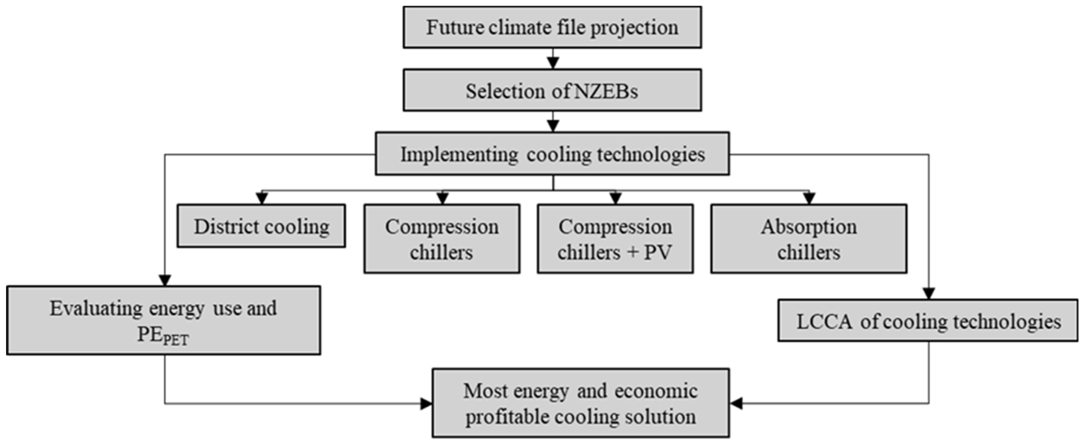
2.1. Framework

The studied district, Näringen in Gävle, is located in central Sweden and it is planned to be a residential district [31] consisting of 6000 new apartments and public service buildings, such as schools. The district is planned to be built between 2025–2050, starting the construction phase in 2025. Six different building models were chosen as representatives to be constructed in the area. The model buildings meet NZEB requirements and these were adapted from a report by Energiforsk [54], a research and knowledge institute that conducts and coordinates energy research in Sweden. Some of the represented models have been constructed in newly utilized neighboring districts [55,56]; however, these must be modified to match the NZEB expectations for the studied future district. Figure 1 depicts the representative building models. The prototype buildings were modeled in IDA-Indoor Climate and Energy (ICE) version 4.8 [57]. The software has been validated using the BESTEST procedure [58]. It has also been validated against measured data [59,60]. More information regarding the validation processes can be found in [61].

Since the district is expected to be fully utilized after 2040, the climate file representing the mid-term future was used to describe the dynamic behavior of the buildings. A typical meteorological year (TMY) file containing 8760 h derived from multiyear data was assembled. The European Coordinated Regional Downscaling Experiment (EURO-CORDEX) was used to assemble the climate file. Data were downloaded from the Earth System Grid Federation (ESGF) [62]. The average annual dry-bulb temperature will be 8 °C whereas it is 5.8 °C at present [63]. July and December are the warmest and the coldest months. Average monthly temperatures for these months correspond to 20 and −1 °C respectively.

To address the aim of the study, a framework has been developed. The workflow to evaluate the economic and energy performance of different employed technologies is shown in Figure 2.

After assembling the future climate files and obtaining the prototype models that are planned to be built in the district, different cooling technologies as shown in Figure 2 were chosen to be assessed from primary energy number and economic perspectives. Finally, the most energy-efficient and profitable cooling solution will be reported.

Three different space cooling technologies were chosen to evaluate their performance for all the building models under same conditions. District cooling (DC), compression chillers coupled with solar photovoltaic (PV) systems (denoted as Chiller + PV) and uncoupled with a PV system, and finally, absorption chillers (Abs) driven by district heating were the cooling technologies considered in this study. The case of compression-only chillers was considered to evaluate the effects of PV systems on the electricity use for cooling, since PV systems are expected to reduce electricity use by employing self-produced electricity that leads to reduction of carbon emissions.

Given that the energy demand is predominantly heating, as district heating (DH) is the most widespread alternative in Sweden in more than 90% of multifamily buildings [64], the new district will have DH for space and domestic hot water heating. Therefore, DH will cover all heating demand irrespective of cooling options. Multifamily buildings are required to have mechanical ventilation systems according to building regulations, whereof systems with a heat exchanger involving heat recovery are common. This study assumes, independently of cooling source, that supply air is chilled by means of a cooling coil to meet the cooling demand (see [20] for more details). The energy efficiency of the heat exchangers was assumed to be 85%. Moreover, in the economic analysis, the costs of transfer of cold from the chiller unit to supply air has been omitted, i.e., assumes these are of the same order of magnitude. The cost differences studied between the technologies are in energy price, purchase of the cooling device, and the physical space these occupy. More details are described below on the cooling alternatives within the scope of this study.

2.1.1. Cooling Alternatives

District cooling is chosen as the first cooling choice. The local energy provider in the studied city, Gävle Energi AB [65], utilizes free cooling from a river and it is responsible for the operation and maintenance of the central compression chillers of the DC system. In this system, water in the network is cooled with the help of the river and if the temperature of the cold source (the river) is higher than 6 °C, two central compression chillers are utilized [66]. In the new district, heat for both space and domestic hot water is obtained from DH; therefore, laying the cooling pipes along with heating pipes at the construction stage of the district is easier and inexpensive. Considering the 4th-generation district heating (4GDH), the return pipes can be used even for a district cooling system, which reduces the investment costs [67]. The energy efficiency ratio (EER) of the central chillers is generally higher than that of the in-house chillers used in the central units in Stockholm with EER 6 [68]. Nevertheless, based on the information obtained from Gävle Energi AB, the EER of the central chillers is 4. Gävle Energi AB uses the nearby river for free cooling; therefore the EER of the systems tend to be lower than those of Stockholm, which has access to more free cooling via the Baltic Sea. The EER under standard rating conditions is defined as the ratio of the total cooling capacity [kW] to the effective input power to the device [69,70].

In this case, buildings are individually connected to the DC network and an installation cost is charged upon connection, based on the power, energy use, and location of the district.

Compression chillers with and without PV systems are chosen as a second cooling alternative. Chiller + PV is expected to be a common solution in the future and the excess PV-produced electricity can be delivered to the grid. This combination was chosen since it encourages self-electricity use, which consequently helps reduce GHG emissions to be on track with the EU commission goals. The panels help in producing the electricity for the compression chillers as it is concluded to be an efficient solution [27]. Apart from that, the impact of climate change on PV generation has been overall reported to be low [71]. To maximize the self-consumption of electricity produced from the PV system, different sizes were evaluated. Panel-to-roof area ratios of 100% and 50% and a panel-to-floor ratio of 10% were considered as the sensitivity analysis cases. Full self-use with minimized imported energy (electricity) could not be achieved and, as mentioned in [72], this is impractical as oversized PV systems are required. A ratio of 10% of floor area appeared to be the optimized ratio as it increased self-use from an average of 20% to 40% compared to the other two. The produced electricity when considering 100% panel-to-roof area is mostly sold to the grid, which is not an optimal choice since more self-use is encouraged. Therefore, a panel-to-floor ratio of 10% was used throughout the rest of the study.

The obtained cooling peak power demand ranges from 4–31 kW for the smallest to the largest models. The compression chillers are chosen from products manufactured by Carrier [73] to meet the cooling demand of the buildings. Two variable speed compression chillers, 17 and 21 kW in nominal cooling capacity, were found suitable to meet the cooling energy demand of the buildings. The number of buildings attached to each chiller and the building’s cooling demand are shown in

Table 1. Number of compression chillers and absorption chillers along with the chosen cooling capacity for the studied models.

		Compression Chiller		Absorption Chiller
Model	Number of Buildings	Capacity (kW)	Number of Systems	Capacity (kW)	Number of Systems
1	4	17	1	17	1
2	12	17	6	35	3
3	18	21	9	35	6
4	20	21	10	17	5
				35	5
5	39	17	39	35	19
6	53	17	106	17	106

. This means that the chiller units may be shared among various buildings, especially depending on building size.

The solar panels were sized based on the available products from SVEA SOLAR [74], a company that is one of the major producers of solar panels in Sweden. The system cost (including the panels, material, financing cost, permits, etc.) was projected based on a report from [75] and it is estimated to be around 10 SEK/W_p (1 EUR/W_p) in 2040s [76]. SEK stands for Swedish crowns. Based on the statistics presented by the European Central Bank [77], 1 euro has been equivalent to 10 SEK over the past years. This rate is considered in this study. The extra electricity produced was considered for sale to the grid at spot price of Nord Pool for Sweden. Data for the spot price is available over the past decade from [55]. The spot price for the analysis was calculated using a moving average with 3 intervals as the prior points to obtain the moving average, since fluctuations in the spot price do not allow obtaining a value by the normal averaging technique.

Finally, absorption chillers are implemented. These chillers use heat as their source of energy and these could be employed both for large buildings and in the central plant of DC system [78]. District heating (DH) has been the main form of heat supply for space heating and domestic hot water and it is expected to be available in the future as well. Therefore, absorption chillers were appropriate options given that DH is the most common form of heating in Sweden [37]. District heat is relatively clean and cheap as it uses mostly recycled heat (for production mix see Section 2.2.3). The emission factor for district heating has shown a large reduction over the past decade with an emission factor of 37 gCO₂ eq/kWh in 2010 to 4 gCO₂ eq/kWh in 2021 for Gävle [65] and it is expected to decline further. Apart from that, the heat generated during the summer can be utilized to provide cooling. The chillers in this study were chosen from Yazaki and their cooling coefficient of performance COP is reported 0.7 [79]. Two absorption chillers, SC5 and SC10, with a 17 kW and 35 kW cooling capacity respectively, were chosen. The number of chillers and required cooling capacity for buildings are shown in Table 1.

2.1.2. Energy Performance of the Buildings

This section is designed to evaluate the changes in PE_PET. The prototype buildings adopt the latest available construction features from the newest city district in the same city [80]. The building specifications are shown in

Table 2. Construction and general specifications of the buildings.

Parameter	Values	Parameter	Values
Uvalues Windows (W/(m2·K))	0.92	Heating set-point [81]	21 °C
Uvalues External walls (W/(m2·K))	0.1	Cooling set-point	25 °C
Uvalues Roofs (W/(m2·K))	0.06	Heat exchanger efficiency	0.85–0.9
Window to floor ratio (%)	10	Number of residents [81]	1.42–2.18
Total area (m2)	400–4000	Internal heat gain (kWh/m2 per year) [82]	25–28

. Appliance and occupant gains, lighting and building properties were chosen from Swedish building regulations and standards for building energy performance [30,81,82], where the latter reference implies 30% lower heat gains from modern household appliances than the older standard. Automatic blinds were added between the windowpanes. Blinds are drawn when the incident solar radiation exceeds 100 W/m² (1500 lx) on the outside of the glazing.

For a building to be considered an NZEB, the condition PE_PET < 75 kWh/m² based on the annual purchased energy must be satisfied. PE_PET is used for the evaluation since lower delivered energy does not necessarily imply lower primary energy (PE) use [26]. Equation (1) represents the calculation flow for PE_PET.

$$P{E}_{PET}=\frac{{{\displaystyle \sum }}_{i=1}^6\left(\frac{E_{heating,i}}{F_{geo}}+E_{cooling,i}+E_{DHW,i}+E_{el,i}\right)\times W{F}_i}{A_{temp}}$$

(1)

where:

$P{E}_{PET}$ Primary energy number, kWh/m² per year

E_heating Energy for heating, kWh per year

F_geo Geographical adjustment factor

E_cooling Energy for cooling, kWh per year

E_DHW Energy for domestic hot water, kWh per year

E_el Building operational electricity use, kWh per year

WF Weight factor

i Index denoting energy carrier type

$A_{temp}$ Heated floor area, m²

The geographical and weight factors are based on the National Board of Housing, Building, and Planning regulations. F_geo for the studied city corresponds to 1.1 and weight factor WF for district heating, district cooling, and electricity are 0.7, 0.6, and 1.8, respectively [30]. It is noteworthy to keep in mind the difference between the term “zero energy building” and NZEB (used in this project). The Swedish definition of “zero energy building” demands on one hand the fulfillment of Swedish passive house criteria and on the other hand a building’s zero energy balance in terms of import or export over a year [83].

2.2. Life Cycle Cost Analysis (LCCA)

LCCA is the economical assessment tool that is used to evaluate the economic performance of the different space cooling technologies studied. LCCA is generally employed to support the decision when there are alternatives to choose from [37]. The net present value (NPV) method is implemented to evaluate the economic performance of the alternative technologies. Equation (2) defines the requirements to implement LCCA for this method. The steps to evaluate and analyze the life cycle cost are from [37,84].

$$LC{C}_{TOT}=I_0+LC{C}_{energy}+LC{C}_{maintenance}-residual value$$

(2)

where $LC{C}_{TOT}$ is the total life cycle cost, $I_0$ is the initial investment, $LC{C}_{energy}$ is the energy cost, and $LC{C}_{maintenance}$ is the maintenance cost. The residual value is the amount that is considered for parts of the system with extended life to meet the duration of the considered service time by assuming a replacement of these parts during the life cycle period. $LC{C}_{maintenance}$ was found to be on average 5% of the investment cost for the in-house solutions and zero for the DC since it is already included in its price and maintaining this system is up to Gävle Energi AB. The residual value was considered to be zero.

The entire life cycle cost of a product or building during an expected life period is estimated with the help of a chosen discount rate. The discount rate is referred to as the interest rate used to determine the present value of future cash flows in discounted cash flow analysis. The real discount rate (d) can be calculated from Equation (3).

$$d=nominal discount rate-inflation$$

(3)

Energy price increases or decreases at an estimated rate different from price inflation even if the energy use is the same from year to year. Equation (4) depicts the real energy price escalation (e).

$$e=Energy price escalation-inflation$$

(4)

In order to make comparisons between present and future costs, the present value must be calculated to convert the costs during the studied period at a discount rate [85]. To be able to compare the costs that occur at different stages and periods of a project, all costs are discounted to the present value. To carry on the calculations, the following two basic factors are considered:

Single present value (SPV), which is used when a cost occurs in a certain year (t) and the cost is discounted then is recalculated with regard to the discount rate to a present value. SPV is calculated based on Equation (5a).

$$\mathrm{S}\mathrm{P}\mathrm{V} \left(d;t\right)=\frac{1}{{\left(1+d\right)}^t}$$

(5a)

Uniform present value (UPV), which is the current value of a future sum of money or series of non-uniform annually recurring amounts over n years, given a specified escalation rate. It is represented in Equation (5b).

$$\mathrm{U}\mathrm{P}\mathrm{V} \left(f;n\right)=\frac{{\left(1+f\right)}^n-1}{f·{\left(1+f\right)}^n}$$

(5b)

where f is the net discount rate. It is presented as in Equation (6) and it includes the price escalation:

$$f=\frac{\left(d-e\right)}{\left(1+e\right)}$$

(6)

2.2.1. Analysis Period

The analysis period was chosen to be 25 years for the absorption and compression chillers based on the general lifespan of the cooling system. This also matches the criteria from [86] from the Federal Energy Management Program which state that the service period is commonly set the same as the life of the system alternative. This period meets the maximum beneficial service period of 40 years. However, the lifespan for the DC system is generally 50 years due to the infrastructure of this system (the piping, etc.). Control systems and the heat exchangers are to be changed after 25 years. Therefore, the analysis period for the DC system also was considered 25 years, and the rest (the infrastructure cost) is counted as the residual value.

2.2.2. Inflation and Discount Rates

The average inflation rate in the past ten years has been 2.18% with the highest rate being 3.87% in 2021 and the lowest being −0.31% in 2014 [87]. The goal, based on the Central Bank of Sweden, is to keep the inflation rate at 2% [88]. However, the inflation rate is omitted by analyzing the real discount and price escalation rates.

The discount rate for the EU members, according to Building Performance Institute of Europe (BPIE), is between 1% and 7% [89]. In order to consider uncertainties in this study, three real discount rates of 3, 4 and 5% were chosen for sensitivity analysis based on [37].

The energy cost and price escalation were retrieved from a report by the Swedish Energy Agency [90]. Different electricity price scenarios have been considered in the report and are shown in Figure 3. Five scenarios are presented in the report as well as several sensitivity analyses. Three of these scenarios are presented as a basis for climate reporting from the Climate Reporting Ordinance [91,92] which places demands on those scenarios that will form the basis for the calculation of greenhouse gas emissions. Scenario reference EU is used for emission calculations for the EU Commission. The scenarios for lower energy prices and lower economic development for gross domestic product (GDP) have been developed corresponding to high and low GHG emissions respectively. Based on the Climate Reporting Ordinance demand, these are further used as a basis for the emission calculations.

Electrification is the scenario developed with an increased degree of electrification compared to other scenarios; In addition, various sensitivity analyses have been performed for this scenario by the Swedish Energy Agency.

To carry out a sensitivity analysis on energy prices, three scenarios representing low, medium, and high price increases, namely lower energy price, reference EU, and electrification, were respectively chosen. The price escalation rate was estimated to be around 1–2% based on the differences in the prices for the mentioned scenarios. However, to cover a wider range of price increase, 0% in changes also was considered. Based on the report published in 2021 from [93], which surveys Sweden’s municipalities and thus makes it possible to compare costs, yearly changes in DH price for the studied city was observed to be less than 1% in the past decade. Therefore, to examine all the scenarios and price escalation rates, different scenarios as shown in

Table 3. Scenarios for energy price escalation based on the respective energy carriers.

Scenarios	Carrier	Price Escalation	Carrier	Price Escalation
Sc 1	El&DC	1%	DH	0%
Sc 2	El&DC	1%	DH	1%
Sc 3	El&DC	2%	DH	0%
Sc 4	El&DC	2%	DH	1%

were considered.

2.2.3. Energy Cost

The DC energy cost was calculated based on the prices from Stockholm Exergi [68] for buildings using less than 50 kW cooling power. Based on the provided calculation procedure, a constant fixed price of 310 EUR and power price of 91.8 EUR/kW must be paid annually apart from the energy price (0.046 EUR/kWh for June–August). The values were taken from Stockholm Exergi since DC is already employed for residential cooling purposes in Stockholm; however, it has not yet been employed in Gävle.

A connection cost must be paid upon connecting the buildings to the system, for which the price is provided by Gävle Energi AB [65]. However, a cost for the heat exchangers and the control system has to be considered in the initial investment (I₀). This value is considered from [94]. It is noteworthy that the connection cost is assumed to be distributed over a span of 50 years, corresponding to network lifespan. Therefore, using the SPV method and considering half of the connection cost (half of the actual lifespan, 25 years), a residual value was obtained. This is carried out to maintain a fair assumption among the considered cooling technologies.

The energy cost for the compression chiller as the in-house cooling technology is calculated based on the cost of electricity. This cost was evaluated based on Gävle Energi AB’s [65] structure for the total electricity price which accounts for the transfer cost, spot price, and energy tax. As mentioned earlier, data for the spot price and the energy tax prices over the past decade are available from [55] and were projected for the mid-term future, corresponding to 3.6 and 4.8 EUR/kW respectively. These prices are projected based on the moving average method projection. The electricity transfer cost corresponds to 0.014 EUR/kWh including VAT (which is 25%).

To calculate the energy cost for absorption chillers as the other in-house cooling technology, DH was considered. DH energy cost was calculated from the provided price list from Gävle Energi AB [65] for each season. The heat delivered to the buildings from Gävle’s DH system consists mostly of recycled heat, corresponding to 60% residual waste heat from industry, 25% heat from combined heat and power plants depending on biofuels, and the rest is heat from flue gases [41]. DH prices correspond to 0.047 EUR/kWh for winter (January–March, November–December) and 0.040 EUR/kWh for autumn (April–May, September–October) and 0.015 EUR/kWh for summer [65].

3. Results and Discussion

3.1. Energy Performance of the Buildings

In this section the authors tried to map the cooling demand of each of the building models and evaluate PE_PET. The implemented climate file represents the mid-term future (2041–2060) since the district is to be utilized from 2040 onward. On average, the amount of annual property equipment electricity and cooling and heating demand for the buildings corresponds to 3.8, 3.4, and 40.7 kWh/m², respectively. The equipment electricity is the operational electricity related to the building’s energy need. The heating and electricity use were not depicted in this section as these are out of the scope of the paper.

For the sake of comparison between the considered cooling technologies, the system boundary is set at building level and since the central chillers on DC will be outside of this boundary, the cooling demand of each model is considered for the calculations for the DC system. This implies that the EER of central chillers of the DC system are not considered in the calculation processes.

Results of the simulations for each of the prototype buildings and their respective used energy for cooling during June–August are shown in Figure 4 (left). Used energy is defined as the amount of energy delivered to the distribution system of the building by the plant or the heat generation or heat removal devices [95]. Since PE_PET is reported based on heated floor area, the used energy and the rest of the investigated parameters related to energy use of the buildings also are reported in this manner. Figure 4 (right) depicts estimated primary energy use over the cooling period (June–August) for each model and the implemented cooling technologies. In order to consider the estimated primary energy use for the cooling season, WFs from the National Board of Housing, Building, and Planning regulations [30] for electricity and district cooling, as mentioned in Section 2.1.2, are considered here.

To investigate the changes in PE_PET when taking away the PV systems, Chiller without PV (denoted as Chiller), is depicted next to Chiller + PV. The used energy to meet the cooling demand for DC is on average 5.0 kWh/m² from thermal energy; this value corresponds to 0.5 and 1.3 kWh/m² for Chiller + PV and Chiller, respectively, in terms of electricity. In the case of Chiller + PV, PV systems are considered a complement to the in-house compression chillers to reduce the electricity use from the grid to obtain a lower primary energy use as compression chillers rely solely on electricity. The produced electricity for calculation purposes in this study is first assumed to be used for cooling purposes, the remainder of which is used for equipment; finally, the excess will be sold to the grid. Equipment electricity and cooling systems were chosen as the main consumers of the produced electricity since these factors are used in PE_PET calculation based on Equation (1). According to the NZEB definition and bounding conditions, these mentioned values must be maintained at a lower value to keep PE_PET < 75 kWh/m² [30].

As indicated in Figure 4, both energy use and primary energy use for the cooling season shows higher value for the absorption chiller and lower value for Chiller + PV for each model. Given the lower cooling COP of 0.7 for the absorption chillers, the used thermal energy for cooling is on average 7.0 kWh/m². In the case of Chiller + PV, the electricity produced by the PV installation helps in reducing the energy used for cooling.

From the obtained results of Figure 4 (right), it can be concluded that the weighting factor that is considered for DC systems underestimates the EER value. WF is 0.6 for DC and lower WF in the order of magnitude of 0.3 can be assumed for the DC system considering the possible available free cooling in DC networks [96], implying that the blue DC bars in Figure 4 (right) would be halved. Moreover, using higher WF values implies an inferior performance by the DCs central chillers, where water with colder temperatures than ambient air is used for heat rejection. This is seen as a gap in the policy-making procedures. Further detailed discussions about these factors will be considered in the authors’ future work.

Figure 5 shows the result for PE_PET. As discussed in the Method section, different forms of energy use in the building are considered in the calculation of the PE_PET, thereby making it a comprehensible parameter in comparing and evaluating the energy use in buildings. However, in terms of DC, the national value of weighting factor 0.7 can be doubted since the local situation would imply 0.45 when using compression chillers without free cooling.

By looking at the depicted result, it could be concluded that from the energy demand perspective, Chiller + PV indicates an optimal combination. This is concluded from the lower PE_PET compared to the other cooling alternatives. By comparing the two technologies, Chiller + PV and Chiller without PV, we can see that the PV system helps in reducing the PE_PET by on average 13%. However, from the cost perspective the system must be analyzed as well.

The influence of energy units on reporting the energy use of the buildings has been previously discussed by some researchers. Stephan et al. [97] have concluded that measuring energy efficiency of buildings per meter of floor area favors the larger buildings. Carlander et al. [98] utilized indicators kWh/(m² × hpers) (hpers = hours of use) and kWh/m² and concluded the former benefits buildings with high occupancy and low electricity use and the latter benefits buildings with low internal heat gains. Therefore, the importance of unit indicators plays a role when it comes to measuring energy efficiency of buildings. However, as was mentioned earlier, since the goal is to measure PE_PET, all units reporting energy demand are reported in kWh/m².

The influence of the shape factor (SFv) of the building also was considered to evaluate the effect of the geometry of the building on the PE_PET. The definition and impact of the shape factor on energy use of buildings is defined by Carpio et al. [99]. They defined SFv as the ratio of the enveloping surfaces to the volume and it is directly related to the heating energy demand in buildings. Energy exchange with the outside is increased if the surface of the building in contact with the outside is more significant. This may be beneficial or unfavorable in certain types of climates. This factor corresponds to 0.74 and 0.54 for models 1 and 2 respectively. For the rest of the models, this value is on average 0.41.

3.2. Life Cycle Cost Analysis

The overall result of this section helps in choosing the economically optimized cooling alternative for the prototype buildings. Detecting the energy-optimized technology or solution may not always be practical due to costs and expenses. This step is taken to make sure that the introduced solution as an energy-optimized technology is also economically acceptable.

The result of the LCCA for different cooling technologies, scenarios, and discount rates are shown in Figure 6. The LCCA result is depicted on the primary axis and the secondary axis depicts the energy use (kWh/m²). The investment (EUR/m²) has been highlighted with a transparent gray box on the bars for each technology and model; therefore, the unhighlighted part depicts the reoccurring values or the net present value. Since the chillers for the DC are central and only require a heat exchanger at the site, the extra cost to consider a utility room for the chillers and the respective installations in the buildings can be excluded for this cooling technology. On the other hand, the compression and absorption chillers are considered the in-house cooling alternatives; therefore, a utility room for all the equipment must be considered. The rental cost for the room was taken from [55] and it is estimated to be around 200 EUR/m² (i.e., as a loss of income). The size of the utility rooms was considered to be around 10 m² based on the required dimensions in catalogues from Yazaki [79].

As indicated in Figure 6, overall, Chiller + PV shows the lowest life cycle cost at the end of the studied period (25 years). At a discount rate of 3%, employing DC as a cooling alternative has from −11 to 35% different life cycle cost compared to Chiller + PV on average for all the scenarios and the studied models. This range corresponds to −10 to 41% and −8 to 47% for discount rates 4 and 5%. For absorption chillers, the range corresponds to on average 2–66% for discount rates of 3, 4, and 5%. The negative values depict lower LCC than that of Chiller + PV’s.

The higher discount rate depicts lower present value of the future cash flows, which can imply that lower discount rates give more value for future reduced operational costs. It could be concluded from Figure 6 that the LCC follows the same trend as that of the energy use; i.e., smaller floor areas correspond to higher life cycle costs as can be seen for models 1 and 2 for all the scenarios and discount rates. These models are the smaller buildings with 400 and 945 m² respectively. Higher costs are associated with these buildings since the investment cost and energy use relative to floor area for these buildings will be higher and, as mentioned earlier, the unit indicator kWh/m² favors buildings with larger conditioned areas. The shape factor for model 1 corresponds to 0.74, which is the highest among the other studied models, and therefore the energy exchange with the outside increases. On the other hand, the area and shape factor for Model 6 correspond to 3925 m² and 0.41 respectively. Therefore, LCC for smaller buildings appear to be higher than the buildings with larger floor areas. Additionally, the initial costs are larger relative to floor area for smaller buildings in relation to the larger buildings. Moreover, the size of chiller and the utility room influence the LCCA for the Chiller + PV and absorption chiller. Since these two cases are regarded as in-house alternatives, the focus on sizing the systems was to try to employ a chiller for each building.

Gävle Energi AB provides the district cooling, which is mainly powered with the help of the nearby river for free cooling purposes. Auxiliary central compression chillers are employed when the temperature of the river is above 6 °C [65] and the river is also used for rejecting heat as opposed to using ambient (warmer) air. Therefore, the energy provider is responsible for the maintenance of the system and generally, DC systems as mentioned earlier tend to have a longer life cycle period (generally 50 years). However, in this study to maintain the consistency among the studied cooling technologies, life cycle period was considered the same for all the systems and the remainder of the connection cost was calculated as residual value (see Equation (2)). On the other hand, as depicted in Table 1, in most of the models, more than one building is connected to the compression or absorption chillers, which helps reduce the investment cost per building since using just one chiller for each building would lead to oversized equipment. However, for DC, each building must be individually connected to the system, which in return affects $LC{C}_{TOT}$ due to its higher investment cost.

The impact of price escalation on probability of different cooling technologies is also depicted in Figure 6. At a 3% discount rate, DC has the highest life cycle cost for different scenarios. Scenarios were defined in Table 3. As depicted in Figure 6, scenarios 1 and 3 depict the lowest life cycle costs. Increasing the DH price escalation from 0% to 1% in scenarios 2 and 4, DC and EL from 1% to 2% in scenarios 3 and 4 increase the LCC compared to scenario 1. Therefore, scenario 4 has 6–10% higher life cycle costs compared to scenario 1 for the studied models, which is the highest range among the studied scenarios. Scenario 2 has 4–7% higher LCC compared to the first scenario. However, this range corresponds to 2–3% for scenario 3. In scenarios 2 and 4, DH has the dominant role as the price during winter (January–March, November–December) and autumn (April–May, September–October) are 0.47 and 0.040 EUR/kWh [51]. However, the cost during summer is 0.015 EUR/kWh, which is a point in favor of the absorption chiller. Apart from the energy price, the investment cost also is taken into consideration, the same way as DC. Therefore, DH has relatively high LCC compared to electricity and cooling life cycle costs.

The investment for DC and Abs is higher than Chillers and Chiller + PV. This value corresponds to up to 40% and 50% of the total life cycle cost (for the smaller models) for DC and Abs respectively. On the other hand, the investment corresponds to maximum 20% of the total life cycle cost for Chiller + PV (for the smaller models). As can be noticed from Figure 6, the reoccurring cost is higher for the Chiller + PV and Chiller. It could be concluded that by a change of policies and reduction of investment cost for DC and Abs, these technologies can be quite competitive with the Chiller + PV.

On the positive side, investment cost for the utility room is not required for the DC, given that it is fitted in the DH space. Utility rooms are regarded as wet rooms and need extra flooring and insulation to prevent damp, noise, and vibration transfer to the residential parts of the building and electric wiring. In contrast, DC is quite hassle-free for the building owner without requiring payment for the maintenance cost other than the annual subscription fee and DC has quite unlimited lifespan. Overall, it can be concluded that high investment costs yield to higher life cycle costs. Additionally, service costs that arise for the two in-house solutions and extra piping between buildings that are sharing cooling units have been neglected. Comparing discount rates of 3–5% for each price escalation scenario, it could be concluded that the lower discount rate gives higher future energy cost in comparison to the investment cost. This aligns with the findings from Khadra et al. [37]. To allow conversion of future costs at present value, discounting of the payments and income streams play an important role. Within this frame, harmonization of the costs at present and future within an economic assessment is made possible [89].

In order to evaluate the effect of the PV system on the LCCA, a case without a PV system coupled to the compression chiller was considered. Figure 7 depicts the difference in LCC between Chiller + PV and Chiller without PV system for scenario 1 as a representative. Removing the PV systems increases the LCC by almost 13% on average for all the models. The differences in the LCC between the Chiller + PV and Chiller are quite small since the saving from the produced electricity from the PVs have to finance its own investment cost. The PV systems play important role on the national level since the electricity sold to the grid allows hydropower and biofuels to be stored for the heating season; however, these may not appear economical for the tenants given the high investment cost and low spot price. The spot price considered for the electricity sold to the grid is calculated based on historic prices, which correspond to 0.036 EUR/kWh, which is a relatively low value, given the recent substantial changes in electricity price due to geopolitical changes. However, due to the mentioned reason, it is expected to have a higher spot price leading to more income from the electricity sold. It is noteworthy that no subsidies were considered for the PV systems either.

Moreover, it can be noted that the difference between Chiller + PV and Chiller are more significant with low discount rates. As mentioned before, lower discount rates give more value for future savings.

Overall, based on the provided results in this section and Section 3.1, compression chillers coupled with PV systems appear to be the optimal choice in both energy and economic aspects. This could be depicted from PE_PET and LCC from Figure 5 and Figure 6 respectively. However, as mentioned earlier, Abs and DC have high investment and lower reoccurring (SPV) values compared to the compression chillers. Therefore, with reduction in the investment, these appear to be competitive technologies.

3.3. Techno-Economic Evaluation of the Studied Cooling Systems

To touch upon the resilience aspect of the studied technologies, several characteristics, such as adaptive and restorative capacities as well as the recovery speed [51] have been looked upon in this section. The adaptive and the restorative capacities of the studied systems can be questioned in extreme ambient temperatures or heatwaves. Outdoor conditions such as temperature and humidity can affect the energy performance of the chillers. In this regard, compression chillers provide higher adaptive capacity compared to absorption chillers [51]. On the other hand, the DC system also possesses the ability to be incorporated with single or multiple cooling technologies in the central plant apart from the free cooling or other environmentally sustainable methods that can act as a heat sink or cold source [66,100] which helps increase the adaptive capacity. It is noteworthy to mention that if an increase in the cooling power is required, the whole unit for the in-house technologies must be changed; however, for the DC system, it is mostly sufficient to change the heat exchanger.

From the refrigerant point of view, absorption chillers and DC are more environmentally sustainable since the chillers employ eco-friendly fluids such as water and these are partially activated by thermal energy. DC can employ free cooling sources.

These studied systems cannot operate without power input. To compensate, these can integrate a local power production such as PV systems or energy storage units such as batteries to increase the resilience. Nevertheless, the space that the PV systems or the storage units occupy cannot be neglected, especially when considering an in-house alternative as the tenants might be obliged to bear the rental costs.

From the input source perspective, the major benefit of the absorption chiller is its operation scheme that can be carried out with a low-grade heat source such as waste heat similar to that of the studied district heating system in this project. Therefore, electrical energy can be reduced, resulting in lower carbon emissions. However, the system might need an additional heating source in case the provided primary source of heat is not sufficient to provide stable operation [51] which may need more development, given that they require district heating temperatures that are relatively high, especially during the non-heating seasons. DC systems also can benefit from free cooling technology and help in reducing the peak power demand, although 100% free cooling during high outdoor temperatures and heatwaves is not possible; therefore, other active cooling technologies must be employed in the system to provide the required cooling. It is notable that DC can reduce the peak demand, thereby reducing electricity use and GHG emissions. From the obtained results, DC appears to be an agreeable cooling technology for buildings with large floor areas. The system does not require spacious utility rooms; therefore, the extra space and the associated rental as well as the system maintenance costs are excluded for the tenants. As mentioned earlier, DC has a longer life cycle, it is hassle-free for the building owner, and, in the case of the studied district, free cooling was employed, which helps reduce the carbon emission and primary energy.

On the other hand, the other cooling alternatives require utility rooms. The extra cost for in-house cooling technologies, in terms of space and its associated investments such as extra insulation, flooring, dampers to reduce noise and vibrations, etc., were neglected to prevent complications in the calculation procedure, but instead considered to be a loss of income corresponding to the rent. Moreover, considering material and related investment costs adds more to the uncertainties. Based on a study carried out by Alrwashdeh et al. [101], both compression chillers and absorption chillers are effective when regarding the benefits over the total cost. However, compression chillers are easily available on the market and they have lower investment and operation costs. These systems also offer a wider range of nominal cooling sizes compared to absorption chillers.

4. Limitations

There are limitations associated with the building type and geometrical configuration. Each apartment was considered as one single zone and the number of occupants and the internal heat gains were all based on Swedish standards. All buildings are residential even though school and commercial buildings also are generally included in districts (450,000 m² are planned for non-residential buildings), which will be covered in future studies. These buildings were excluded to match the definition of the district which is “residential district”. The considered energy prices, such as spot price and energy tax prices, fluctuate on a short-term basis though a constant value was considered for those parameters. The extra investment costs for the utility room when employing an in-house cooling technology were excluded from the calculations and considered as a loss of future rental income. The lifecycle of a DC system was confined to 25 years to attain a coherent result. The sizes available on the market today for the chillers are larger than the demand for each of the smaller buildings. This may involve practical problems when it comes to ownership of various buildings that would have to share a common cooling unit.

5. Future Work

Studies on possibilities and pathways to deep decarbonization have been carried out in Canada [13], France [102], and Greece [103] and were initially intended to be carried out in this study as well; however, due to the extent of the current work, it was decided to postpone the GHG emissions associated with each technology as future work.

6. Conclusions

This paper was framed around a research question that aimed at evaluating different cooling technologies and introducing the more suitable space cooling alternatives from primary energy number (PE_PET) and economic points of view. This was done from both a property developer/owner and an energy supplier perspective regarding a future residential district in Gävle, Sweden. The district is one of the Swedish government’s nine selected initiatives concerning development of future environmentally sustainable districts. The cooling alternatives are district cooling (DC), compression chillers coupled and uncoupled with PV systems, and absorption chillers. Compression chillers without PV systems were considered to evaluate the effect of the PV systems on energy use of the building. PV systems were coupled with the compression chillers to reduce the electricity use of the system, since this is a solution that uses electricity as the energy source.

Primary energy number (PE_PET) was considered based on the Swedish National Board of Housing Building and Planning to represent the energy performance of the buildings. Accordingly, chillers coupled with PV system and absorption chillers had the least and the highest PE_PET among the studied technologies. Chillers alone appeared to be an agreeable alternative after chillers coupled with a PV system with on average 11% higher PE_PET value for the studied models, compared to the optimal case. However, generalized weighting factors may bias use of local chillers instead of central chillers used in DC.

Life cycle cost analysis was considered to evaluate the economic performance of each technology to discover the economically optimized alternative. Discount rates of 3, 4, and 5% as well as four price escalation scenarios were considered as sensitivity studies. Chillers coupled with PV systems appeared to be overall the optimal technology from this perspective. DC appeared to be an agreeable cooling technology for large buildings as it had up to, on average, 10% lower life cycle cost compared to chillers coupled with PV systems for the considered discount rates.

On the other hand, absorption chillers did not appear as an optimal choice either from PE_PET or economic perspective. From the primary energy analysis, the PE_PET value is 20% higher than the optimal technology. Based on the LCCA results, the lifecycle cost ranges from 2–48% higher than the optimal technology, i.e., chillers coupled with PV panels. It is noteworthy to mention that the energy carrier for this alternative is district heating, which is an environmentally sustainable source and mainly uses waste heat. From the electricity grid point of view, the absorption chillers are quite beneficial as there is abundance of unused heat from the district heating system during summer; therefore, the electricity can be exported or saved, given the interconnected grid. The drawback is the high supply and return district heating water temperatures required for efficient absorption heat pump use, thus reducing efficiency for both DH and DHC (district heating and cooling) application.

References

1. UN-Habitat Core Team. Urbanization and Development Emerging Futures; UN-Habitat Core Team: New York, NY, USA, 2016. [Google Scholar]
2. United Nations Division of Economic Development Affairs. World Population Prospects 2019 Highlights; United Nations Division of Economic Development Affairs: New York, NY, USA, 2019. [Google Scholar]
3. Inayat, A.; Raza, M. District Cooling System via Renewable Energy Sources: A Review. Renew. Sustain. Energy Rev. 2019, 107, 360–373. [Google Scholar] [CrossRef]
4. OECD; IEA; IRENA. Perspectives for the Energy Transition: Investment Needs for a Low-Carbon Energy System; IEA Publications: Paris, France, 2017. [Google Scholar]
5. European Commission a European Green Deal|European Commission. Available online: https://ec.europa.eu/info/strategy/priorities-2019-2024/european-green-deal_en (accessed on 27 May 2021).
6. European Commission European Climate Law Climate Action. Available online: https://ec.europa.eu/clima/policies/eu-climate-action/law_en (accessed on 27 May 2021).
7. European Commission European Climate Pact. Available online: https://ec.europa.eu/clima/eu-action/european-green-deal/european-climate-pact_en (accessed on 22 April 2022).
8. European Commission EU Adaptation Strategy. Available online: https://ec.europa.eu/clima/eu-action/adaptation-climate-change/eu-adaptation-strategy_en (accessed on 22 April 2022).
9. European Commission Energy and the Green Deal|European Commission. Available online: https://ec.europa.eu/info/strategy/priorities-2019-2024/european-green-deal/energy-and-green-deal_en (accessed on 22 April 2022).
10. Zappa, W.; Junginger, M.; van den Broek, M. Is a 100% Renewable European Power System Feasible by 2050? Appl. Energy 2019, 233–234, 1027–1050. [Google Scholar] [CrossRef]
11. Pleßmann, G.; Blechinger, P. How to Meet EU GHG Emission Reduction Targets? A Model Based Decarbonization Pathway for Europe’s Electricity Supply System until 2050. Energy Strategy Rev. 2017, 15, 19–32. [Google Scholar] [CrossRef]
12. Heun, M.K.; Brockway, P.E. Meeting 2030 Primary Energy and Economic Growth Goals: Mission Impossible? Appl. Energy 2019, 251, 112697. [Google Scholar] [CrossRef]
13. Vaillancourt, K.; Bahn, O.; Frenette, E.; Sigvaldason, O. Exploring Deep Decarbonization Pathways to 2050 for Canada Using an Optimization Energy Model Framework. Appl. Energy 2017, 195, 774–785. [Google Scholar] [CrossRef]
14. European Commission Official Journal of the European Union L 153. Available online: https://eur-lex.europa.eu/legal-content/EN/TXT/?uri=OJ:L:2010:153:TOC (accessed on 28 May 2021).
15. Latõšov, E.; Volkova, A.; Siirde, A.; Kurnitski, J.; Thalfeldt, M. Primary Energy Factor for District Heating Networks in European Union Member States. In Proceedings of the Energy Procedia, Seoul, Republic of Korea, 4–7 September 2017; Volume 116, pp. 69–77. [Google Scholar]
16. Marszal, A.J.; Heiselberg, P.; Bourrelle, J.S.; Musall, E.; Voss, K.; Sartori, I.; Napolitano, A. Zero Energy Building—A Review of Definitions and Calculation Methodologies. Energy Build. 2011, 43, 971–979. [Google Scholar] [CrossRef]
17. Attia, S.; Eleftheriou, P.; Xeni, F.; Morlot, R.; Ménézo, C.; Kostopoulos, V.; Betsi, M.; Kalaitzoglou, I.; Pagliano, L.; Cellura, M.; et al. Overview and Future Challenges of Nearly Zero Energy Buildings (NZEB) Design in Southern Europe. Energy Build. 2017, 155, 439–458. [Google Scholar] [CrossRef]
18. Cellura, M.; Guarino, F.; Longo, S.; Mistretta, M. Energy Life-Cycle Approach in Net Zero Energy Buildings Balance: Operation and Embodied Energy of an Italian Case Study. Energy Build. 2014, 72, 371–381. [Google Scholar] [CrossRef]
19. Lindkvist, C.; Karlsson, A.; Sørnes, K.; Wyckmans, A. Barriers and Challenges in NZEB Projects in Sweden and Norway. In Proceedings of the Energy Procedia, Trondheim, Norway, 22–24 January 2014; Volume 58, pp. 199–206. [Google Scholar]
20. Sayadi, S.; Hayati, A.; Akander, J.; Cehlin, M. Cooling Demand Reduction Approaches for Typical Buildings in a Future City District in Mid-Sweden. In Proceedings of the Building Simulation 2021, Bruges, Belgium, 1–3 September 2021. [Google Scholar]
21. Wrålsen, B.; O’Born, R.; Skaar, C. Life Cycle Assessment of an Ambitious Renovation of a Norwegian Apartment Building to NZEB Standard. Energy Build. 2018, 177, 197–206. [Google Scholar] [CrossRef]
22. European Commission Official Journal of the European Union L 208. Available online: https://eur-lex.europa.eu/legal-content/EN/TXT/?uri=OJ:L:2016:208:TOC (accessed on 28 May 2021).
23. European Commission Official Journal of the European Union L 81. Available online: https://eur-lex.europa.eu/legal-content/EN/TXT/?uri=OJ%3AL%3A2012%3A081%3ATOC (accessed on 28 May 2021).
24. European Commission Official Journal of the European Union C 115. Available online: https://eur-lex.europa.eu/legal-content/EN/TXT/?uri=OJ%3AC%3A2012%3A115%3ATOC (accessed on 28 May 2021).
25. D’Agostino, D. Assessment of the Progress towards the Establishment of Definitions of Nearly Zero Energy Buildings (NZEBs) in European Member States. J. Build. Eng. 2015, 1, 20–32. [Google Scholar] [CrossRef]
26. Swing Gustafsson, M.; Gustafsson, M.; Myhren, J.A.; Dotzauer, E. Primary Energy Use in Buildings in a Swedish Perspective. Energy Build. 2016, 130, 202–209. [Google Scholar] [CrossRef]
27. Gustafsson, M.; Thygesen, R.; Karlsson, B.; Ödlund, L. Rev-Changes in Primary Energy Use and CO2 Emissions—An Impact Assessment for a Building with Focus on the Swedish Proposal for Nearly Zero Energy Buildings. Energy 2017, 10, 978. [Google Scholar] [CrossRef]
28. Boverket. Konsekvensutredning BFS 2020: Boverkets Föreskrifter Och Allmänna Råd Om Energimätning i Byggnader; Boverket: Karlskrona, Sweden, 2020. [Google Scholar]
29. Häggström, A. Fjärrvärmeburen Kyla TT—Cooling with District Heating (Eng); Department of Applied Physics and Electronics, Faculty of Science and Technology, Umeå University: Umeå, Sweden, 2017. [Google Scholar]
30. Boverket. Konsekvensutredning BFS 2020: 4 Boverkets Föreskrifter Om Ändring i Verkets Byggregler (2011:6)—Föreskrifter Och Allmänna Råd, BBR, Avsnitt 5 Och 9; Boverket: Karlskrona, Sweden, 2020. [Google Scholar]
31. Gävle Kommun the Industry—One of Europe’s Most Sustainable Districts—Gävle Municipality. Available online: https://www.gavle.se/kommunens-service/bygga-trafik-och-miljo/planer-och-samhallsbyggnadsprojekt-i-gavle/pagaende-byggprojekt-i-gavle/naringen/ (accessed on 7 January 2022).
32. Pombo, O.; Rivela, B.; Neila, J. The Challenge of Sustainable Building Renovation: Assessment of Current Criteria and Future Outlook. J. Clean. Prod. 2016, 123, 88–100. [Google Scholar] [CrossRef]
33. Official Journal of the European Union COMMISSION DELEGATED REGULATION (EU) No 244/2012. Available online: http://data.europa.eu/eli/reg_del/2012/244/oj (accessed on 1 May 2022).
34. Villa-Arrieta, M.; Sumper, A. Economic Evaluation of Nearly Zero Energy Cities. Appl. Energy 2019, 237, 404–416. [Google Scholar] [CrossRef]
35. Ferrara, M.; Fabrizio, E.; Virgone, J.; Filippi, M. Energy Systems in Cost-Optimized Design of Nearly Zero-Energy Buildings. Autom. Constr. 2016, 70, 109–127. [Google Scholar] [CrossRef]
36. Bonakdar, F.; Dodoo, A.; Gustavsson, L. Cost-Optimum Analysis of Building Fabric Renovation in a Swedish Multi-Story Residential Building. Energy Build. 2014, 84, 662–673. [Google Scholar] [CrossRef]
37. Khadra, A.; Hugosson, M.; Akander, J.; Myhren, J.A. Economic Performance Assessment of Three Renovated Multi-Family Buildings with Different HVAC Systems. Energy Build. 2020, 224, 110275. [Google Scholar] [CrossRef]
38. Congedo, P.M.; Baglivo, C.; Seyhan, A.K.; Marchetti, R. Worldwide Dynamic Predictive Analysis of Building Performance under Long-Term Climate Change Conditions. J. Build. Eng. 2021, 42, 103057. [Google Scholar] [CrossRef]
39. Sengupta, A.; Al Assaad, D.; Bastero, J.B.; Steeman, M.; Breesch, H. Impact of Heatwaves and System Shocks on a Nearly Zero Energy Educational Building: Is It Resilient to Overheating? Build. Environ. 2023, 234, 110152. [Google Scholar] [CrossRef]
40. TERMO—Värme Och Kyla För Framtidens Energisystem. Available online: https://www.energimyndigheten.se/utlysningar/utlysning-termo--varme-och-kyla-for-framtidens-energisystem/ (accessed on 1 December 2022).
41. Sayadi, S.; Akander, J.; Hayati, A.; Cehlin, M. Analyzing the Climate-Driven Energy Demand and Carbon Emission for a Prototype Residential NZEB in Central Sweden. Energy Build. 2022, 261, 111960. [Google Scholar] [CrossRef]
42. Bakhtiari, H.; Sayadi, S.; Akander, J.; Hayati, A.; Cehlin, M. How Will Mechanical Night Ventilation Affect the Electricity Use and the Electrical Peak Power Demand in 30 Years?—A Case Study of a Historic Office Building in Sweden. In Proceedings of the International Conference on Building Energy and Environment (COBEE 2022), Montreal, QC, Canada, 26 July 2022. [Google Scholar]
43. Ylmén, P.; Schade, J. Termisk Inomhuskomfort Vid Värmeböljor; RISE Research Institutes of Sweden: Borås, Sweden, 2021; ISBN 978-91-89385-21-4.
44. Machard, A.; Inard, C.; Alessandrini, J.M.; Pelé, C.; Ribéron, J. A Methodology for Assembling FutureWeather Files Including Heatwaves for Building Thermal Simulations from the European Coordinated Regional Downscaling Experiment (EURO-CORDEX) Climate Data. Energy 2020, 13, 3424. [Google Scholar] [CrossRef]
45. Cannon, A.J. Multivariate Quantile Mapping Bias Correction: An N-Dimensional Probability Density Function Transform for Climate Model Simulations of Multiple Variables. Clim. Dyn. 2018, 50, 31–49. [Google Scholar] [CrossRef]
46. Cannon, A.J.; Sobie, S.R.; Murdock, T.Q. Bias Correction of GCM Precipitation by Quantile Mapping: How Well Do Methods Preserve Changes in Quantiles and Extremes? J. Clim. 2015, 28, 6938–6959. [Google Scholar] [CrossRef]
47. IEA EBC IEA EBC||Annex 80||Resilient Cooling||IEA EBC||Annex 80. Available online: https://annex80.iea-ebc.org/ (accessed on 31 January 2022).
48. Nik, V.M.; Sasic Kalagasidis, A. Impact Study of the Climate Change on the Energy Performance of the Building Stock in Stockholm Considering Four Climate Uncertainties. Build. Environ. 2013, 60, 291–304. [Google Scholar] [CrossRef]
49. Jylhä, K.; Jokisalo, J.; Ruosteenoja, K.; Pilli-Sihvola, K.; Kalamees, T.; Seitola, T.; Mäkelä, H.M.; Hyvönen, R.; Laapas, M.; Drebs, A. Energy Demand for the Heating and Cooling of Residential Houses in Finland in a Changing Climate. Energy Build. 2015, 99, 104–116. [Google Scholar] [CrossRef]
50. Petersen, S. The Effect of Local Climate Data and Climate Change Scenarios on the Thermal Design of Office Buildings in Denmark. In Proceedings of the IBPSA-Nordic, Oslo, Norway, 13–14 October 2020; pp. 179–186. [Google Scholar]
51. Zhang, C.; Kazanci, O.B.; Levinson, R.; Heiselberg, P.; Olesen, B.W.; Chiesa, G.; Sodagar, B.; Ai, Z.; Selkowitz, S.; Zinzi, M.; et al. Resilient Cooling Strategies—A Critical Review and Qualitative Assessment. Energy Build. 2021, 251, 111312. [Google Scholar] [CrossRef]
52. Moazami, A.; Carlucci, S.; Nik, V.M.; Geving, S. Towards Climate Robust Buildings: An Innovative Method for Designing Buildings with Robust Energy Performance under Climate Change. Energy Build. 2019, 202, 109378. [Google Scholar] [CrossRef]
53. Homaei, S.; Hamdy, M. A Robustness-Based Decision Making Approach for Multi-Target High Performance Buildings under Uncertain Scenarios. Appl. Energy 2020, 267, 114868. [Google Scholar] [CrossRef]
54. Gustafsson, M.; Åberg, M.; Berner Wik, P. Fjärrvärme i Framtidens Hållbara Bostadsområden 2021-812; Energiforsk AB: Stockholm, Sweden, 2021. [Google Scholar]
55. SCB Statistikmyndigheten (SCB). Available online: https://www.scb.se/ (accessed on 17 January 2022).
56. Wik, P.B. Perspectives of a Climate-Neutral Urban District Evaluation of Greenhouse Gas Emissions, Exergy and Energy Balances; University of Gävle: Gävle, Sweden, 2020. [Google Scholar]
57. Equa Simulation Building Performance-Simulation Software|EQUA. Available online: https://www.equa.se/en/ (accessed on 19 August 2020).
58. ANSI/ASHRAE Standard 140-2017: Standard Method of Test for the Evaluation of Building Energy Analysis Computer Programs; ASHRAE Standard: Atlanta, GA, USA; ISBN 1041-2336.
59. Sahlin, P.; Eriksson, L.; Grozman, P.; Johnsson, H.; Shapovalov, A.; Vuolle, M. Whole-Building Simulation with Symbolic DAE Equations and General Purpose Solvers. Build. Environ. 2004, 39, 949–958. [Google Scholar] [CrossRef]
60. Moosberger, S. IDA ICE CIBSE-Validation Test of IDA Indoor Climate and Energy Version 4.0 According to CIBSE TM33, Issue 3 Report 2007-12-17; Hochschule Luzern–Technik & Architektur: Horw, Switzerland, 2007. [Google Scholar]
61. Validation & Certifications—Simulation Software|EQUA. Available online: https://www.equa.se/en/ida-ice/validation-certifications (accessed on 18 August 2020).
62. ESGF ESGF-LLNL—Home|ESGF-CoG. Available online: https://esgf-node.llnl.gov/projects/esgf-llnl/ (accessed on 10 June 2021).
63. Sveby Sveby|Branchstandard För Energi i Byggnader. Available online: http://www.sveby.org/ (accessed on 21 June 2021).
64. Energimyndigheten Energistatistik För Småhus, Flerbostadshus Och Lokaler. Available online: https://www.energimyndigheten.se/statistik/den-officiella-statistiken/statistikprodukter/energistatistik-for-smahus-flerbostadshus-och-lokaler/ (accessed on 23 August 2022).
65. Gävle Energi Gävle Energi AB. Available online: https://www.gavleenergi.se/ (accessed on 4 June 2021).
66. Sayadi, S.; Akander, J.; Hayati, A.; Cehlin, M. Review on District Cooling and Its Application in Energy Systems. In Urban Transition-Perspectives on Urban Systems and Environments; IntechOpen: London, UK, 2021. [Google Scholar]
67. Dahlberg Larsson, C.; Selinder, P.; Walletun, H. Fastighetsanpassning För 4GDH Cilla Dahlberg Larsson; Energiforsk AB: Stockholm, Sweden, 2018. [Google Scholar]
68. Stockholm Exergi Stockholm Exergi. Available online: https://www.stockholmexergi.se/en/ (accessed on 25 June 2022).
69. Official Journal of the European Union Commission Regulation (EU) No 206/2012 of 6 March 2012. Available online: https://eur-lex.europa.eu/eli/reg/2012/206/oj (accessed on 24 April 2023).
70. Park, W.Y.; Shah, N.; Choi, J.Y.; Kang, H.J.; Kim, D.H.; Phadke, A. Lost in Translation: Overcoming Divergent Seasonal Performance Metrics to Strengthen Air Conditioner Energy-Efficiency Policies. Energy Sustain. Dev. 2020, 55, 56–68. [Google Scholar] [CrossRef]
71. Matera, N.; Mazzeo, D.; Baglivo, C.; Congedo, P.M. Will Climate Change Affect Photovoltaic Performances? A Long-Term Analysis from 1971 to 2100 in Italy. Energies 2022, 15, 9546. [Google Scholar] [CrossRef]
72. Cillari, G.; Franco, A.; Fantozzi, F. Sizing Strategies of Photovoltaic Systems in NZEB Schemes to Maximize the Self-Consumption Share. Energy Rep. 2021, 7, 6769–6785. [Google Scholar] [CrossRef]
73. Carrier Carrier Luftkonditionering, Värme Och Ventilation. Available online: https://www.carrier.com/commercial/sv/se/ (accessed on 3 June 2022).
74. Svea Solar Svea Solar—Solar, Chargers, Batteries, Energy. Available online: https://sveasolar.com/ (accessed on 16 June 2022).
75. Global data Rooftop Solar Photovoltaic (PV) Market Size, Share and Trends Analysis by Technology, Installed Capacity, Generation, Drivers, Constraints, Key Players and Forecast. 2021–2030. Available online: https://www.globaldata.com/data/ (accessed on 26 June 2022).
76. Skoczkowski, T.; Bielecki, S.; Wojtyńska, J. Long-Term Projection of Renewable Energy Technology Diffusion. Energies 2019, 12, 4261. [Google Scholar] [CrossRef]
77. Bank, E.C. European Central Bank. Available online: https://www.ecb.europa.eu/home/html/index.sv.html (accessed on 18 April 2023).
78. Amiri, S. Economic and Environmental Benefits of CHP-Based District Heating Systems in Sweden; Energiforsk AB: Linköping, Sweden, 2013. [Google Scholar]
79. Yazaki Yazaki Energy Systems, Inc. Available online: https://www.yazakienergy.com/index.htm (accessed on 3 June 2022).
80. Gävle Municipality Gävle Strand—Etapp 3—Gävle Kommun. Available online: https://www.gavle.se/kommunens-service/bygga-trafik-och-miljo/planer-och-samhallsbyggnadsprojekt-i-gavle/pagaende-byggprojekt-i-gavle/gavle-strand-etapp-3/ (accessed on 7 January 2022).
81. Sveby Brukarindata Bostäder. Branschstandard För Energi I Byggnader; Version 1; SVEBY: Stockholm, Sweden, 2012; p. 28. [Google Scholar]
82. Westin, R. Hushållsel I Nybyggda Flerbostadshus; Skanska Teknik: Hudiksvall, Sweden, 2019. [Google Scholar]
83. Berggren, B.; Wall, M.; Flodberg, K.; Sandberg, E. Net ZEB Office in Sweden—A Case Study, Testing the Swedish Net ZEB Definition. Int. J. Sustain. Built Environ. 2012, 1, 217–226. [Google Scholar] [CrossRef]
84. Petrović, B.; Zhang, X.; Eriksson, O.; Wallhagen, M. Life Cycle Cost Analysis of a Single-Family House in Sweden. Buildings 2021, 11, 215. [Google Scholar] [CrossRef]
85. Gustafsson, M.; Gustafsson, M.S.; Myhren, J.A.; Bales, C.; Holmberg, S. Techno-Economic Analysis of Energy Renovation Measures for a District Heated Multi-Family House. Appl. Energy 2016, 177, 108–116. [Google Scholar] [CrossRef]
86. Kneifel, J.; Webb, D. Life Cycle Costing Manual for the Federal Energy Management Program; National Institute of Standards and Technology: Washington, DC, USA, 2020.
87. Historic Inflation Sweden—Historic CPI Inflation Sweden. Available online: https://www.inflation.eu/en/inflation-rates/sweden/historic-inflation/cpi-inflation-sweden.aspx (accessed on 7 May 2022).
88. Startsida|Sveriges Riksbank. Available online: https://www.riksbank.se/ (accessed on 7 May 2022).
89. Steinbach, J.; Staniaszek, D. Discount Rates in Energy System Analysis; BPIE Fraunhofer ISI: West Bengal, India, 2015; Volume 6, pp. 1–20. [Google Scholar]
90. Energimyndighetens. Scenarier Över Sveriges Energisystem 2020; Energimyndigheten: Eskilstuna, Sweden, 2021. [Google Scholar]
91. Sveriges Riksdag Klimatrapporteringsförordning (2014:1434) Svensk Författningssamling 2014:2014:1434 t.o.m. SFS 2021:1292—Riksdagen. Available online: https://www.riksdagen.se/sv/dokument-lagar/dokument/svensk-forfattningssamling/klimatrapporteringsforordning-20141434_sfs-2014-1434 (accessed on 9 May 2022).
92. European Commissions. Europaparlamentets Och Rådets Förordning (EU) Nr 525/2013; European Commissions: Brussels, Belgium, 2013.
93. Nils Holgersson Nils Holgersson. Available online: https://nilsholgersson.nu/ (accessed on 25 June 2022).
94. Kartläggning av Marknaden för Fjärrkyla. Kartläggning av Marknaden för Fjärrkyla; Kartläggning av Marknaden för Fjärrkyla: Eskilstuna, Sweden, 2013. [Google Scholar]
95. EQUA IDA-Indoor Climate and Energy Support. Available online: http://www.equaonline.com/iceuser/new_documentation.html (accessed on 7 February 2021).
96. Energiföretagen Sverige—Swedenergy—AB. Available online: https://www.energiforetagen.se/ (accessed on 26 March 2021).
97. Stephan, A.; Crawford, R.H. The Relationship between House Size and Life Cycle Energy Demand: Implications for Energy Efficiency Regulations for Buildings. Energy 2016, 116, 1158–1171. [Google Scholar] [CrossRef]
98. Carlander, J.; Moshfegh, B.; Akander, J.; Karlsson, F. Effects on Energy Demand in an Office Building Considering Location, Orientation, Façade Design and Internal Heat Gains-A Parametric Study. Energies 2020, 13, 6170. [Google Scholar] [CrossRef]
99. Carpio, M.; Carrasco, D. Impact of Shape Factor on Energy Demand, CO2 Emissions and Energy Cost of Residential Buildings in Cold Oceanic Climates: Case Study of South Chile. Sustainability 2021, 13, 9491. [Google Scholar] [CrossRef]
100. Schibuola, L.; Tambani, C. Performance Assessment of Seawater Cooled Chillers to Mitigate Urban Heat Island. Appl. Eng. 2020, 175, 115390. [Google Scholar] [CrossRef]
101. Alrwashdeh, S.S.; Ammari, H. Life Cycle Cost Analysis of Two Different Refrigeration Systems Powered by Solar Energy. Case Stud. Therm. Eng. 2019, 16, 100559. [Google Scholar] [CrossRef]
102. Krakowski, V.; Assoumou, E.; Mazauric, V.; Maïzi, N. Feasible Path toward 40–100% Renewable Energy Shares for Power Supply in France by 2050: A Prospective Analysis. Appl. Energy 2016, 171, 501–522. [Google Scholar] [CrossRef]
103. Tigas, K.; Giannakidis, G.; Mantzaris, J.; Lalas, D.; Sakellaridis, N.; Nakos, C.; Vougiouklakis, Y.; Theofilidi, M.; Pyrgioti, E.; Alexandridis, A.T. Wide Scale Penetration of Renewable Electricity in the Greek Energy System in View of the European Decarbonization Targets for 2050. Renew. Sustain. Energy Rev. 2015, 42, 158–169. [Google Scholar] [CrossRef]
Figure 1. The six building models used for evaluating energy use in the future area of Näringen.
Energies 16 03852 g001
Figure 2. Overview of the workflow to evaluate the economic and energy performance of the cooling systems.
Energies 16 03852 g002
Figure 3. Electricity prices and electricity price development for each scenario until 2050 [80].
Energies 16 03852 g003
Figure 4. Used energy for cooling (left) and estimated seasonal primary energy use for June–August (right) for the studied building models and cooling technologies.
Energies 16 03852 g004
Figure 5. PEPET for the investigated space cooling technologies, district cooling (DC), chiller with PV system (Chiller + PV), compression chiller (Chiller), and absorption chiller (Abs) for each of the prototype building models for a complete year.
Energies 16 03852 g005
Figure 6. Life cycle cost analysis (SPV method) for the studied models, discount rates 3, 4 and 5% as well as different price escalation scenarios as depicted in Table 3 (primary axis). Energy use per heated floor area (secondary axis). For district cooling (DC), compression chillers with and without solar panels (Chiller + PV, Chiller) and absorption chillers (Abs).
Energies 16 03852 g006
Figure 7. Changes in life cycle cost analysis (SPV method) when removing the PV systems from compression chillers for scenario 1.
Energies 16 03852 g007