Abstract
A novel energy management system featuring a unique framework involving multiple hierarchical controllers at the distribution and transmission network levels is proposed. The unique objective function of this energy management system is designed to enhance system inertia during black start and optimise load shedding. The objective function further aims to increase reliance on renewable energy sources, prioritising solar power along with battery and fuel cell technologies. This work delves deeply into the dynamics of multi-area power networks, where some areas possess black start capabilities (BSAs) while others do not (NBSAs). The proposed energy management system specifically explores the complex interplay between these black start capabilities and the hierarchical load restoration order. During grid blackouts, the systems located in BSA areas are tasked with first restoring essential loads in their own regions before extending aid to the adjacent NBSA areas, taking into account factors such as their available reserved power and geographical proximity. This work is extended to analyse complex multi-area power network architectures. This extended analysis provides invaluable insights for enhancing power restoration processes and facilitating the large-scale integration of sustainable energy solutions in complex systems. The proposed energy management system is validated using the IEEE 39-Bus network, which consists of ten distinct areas, each differing in their black start capabilities. The results demonstrate the superiority of the proposed system.
1. Introduction
As power systems evolve to incorporate more renewable energy sources, they face new challenges in maintaining grid stability and reliability, especially during critical situations such as black start events and load shedding [1]. The inherent variability of renewable sources, such as solar power, complicates the grid’s ability to quickly and efficiently recover from outages. This variability in renewable generation highlights the need for advanced energy management systems that can effectively handle the complexities introduced by renewable integration. Moreover, these advanced management systems require robust capabilities for planning and performing optimised load shedding to protect critical services during emergency situations. Therefore, advanced energy management involves not only predicting and reducing fluctuations due to renewable sources but also ensuring that power can be rapidly and efficiently redistributed during outages. Consequently, there is a pressing need for ongoing research aimed at enhancing the overall resilience of power grids. This research is essential in addressing the dual challenges of maintaining system reliability in the face of increasing renewable energy integration while simultaneously advancing toward a more sustainable energy future [2].
The literature has explored a variety of optimisation approaches for energy management systems within microgrids. The authors of [3,4] focus on management strategies for electric vehicle charging to reduce costs, but they overlook considerations for black start capabilities and broader network-level implications. Similarly, the authors of [5,6] propose optimising microgrid profits to enhance community welfare, yet they also fail to address the importance of black start capabilities. Efforts are also been made to balance multiple objectives in energy management using complex machine learning algorithms, as demonstrated in [7,8]. However, these studies do not directly address the critical issues of black start capabilities or the inherent complexity of the proposed algorithms. The authors of [9] explore the integration of distributed generators and loads within DC microgrids. This study highlights benefits such as enhanced reliability, reduced emissions, and lower generation costs. Yet, this study requires a complex energy management system to handle the underlying complex, non-convex mixed-integer nonlinear optimisation problem. The authors of [10] investigate extending the lifetime of energy sources, but they do not consider the broader aspects of energy management across different parts of the network. Meanwhile, a broader perspective is adopted in [11,12,13,14], with a shift towards optimal renewable energy integration and its economic implications. Specifically, Ref. [11] proposes a management system to minimise long-term operating costs and enhance grid economic sustainability, but it does not address energy management during severe scenarios. The authors of [14] present a novel two-stage energy management system for small-scale grid-connected systems, such as smart homes, which improves power exchange predictability but does not consider changes to user habits or pricing plans. Similarly, the authors of [12] explore maximising active power reserve in isolated microgrids using nonlinear optimisation, yet they overlook the management of black start recovery alongside renewable resource integration. Lastly, the authors of [13] aim to reduce total operational costs while ensuring resilience under islanding conditions. However, their system fails to consider the prediction of the next day’s renewable energy generation and its variability, as well as the user welfare aspect.
On the other hand, the authors of [15,16,17] broaden the focus on black start capabilities, each contributing different insights into emergency recovery mechanisms. For instance, the authors of [15] enhance the utilisation rate of photovoltaic systems and the state of charge tracking, which effectively manage energy during critical recovery phases. However, they do not address broader energy distribution optimisation challenges at both distribution and transmission levels. Conversely, the authors of [16] tackle key issues such as voltage and frequency support during black start but lack a comprehensive optimisation framework, which limits the energy management capability. Similarly, the authors of [17] focus on minimising voltage and frequency transients but fail to address broader grid management and constraints in their optimisation problem.
In previous energy management systems, a common drawback is the lack of real-time optimisation and consideration for system uncertainties. Consequently, the authors of [18,19] focus on optimising power exchange and managing uncertainty, yet they do not incorporate black start capabilities. Similarly, the studies in [20,21] propose optimising operations and managing stochastic parameters, but they also neglect to address the critical aspects of black start capabilities. The authors of [22] utilise a bi-level iterative optimisation algorithm to minimise various system costs and maximise revenues, including benefits from renewable energy. However, the study fails to address the constraints of both distribution and transmission networks. Finally, the study in [23] focuses on real-time energy management and operational optimisation without taking into account all aspects of the networks, including the distribution and transmission levels, which are crucial for holistic management.
Table 1 provides a detailed comparison of energy management systems as proposed in the literature. It provides a comprehensive analysis of their methodologies, capabilities, and areas of application. A significant limitation of existing energy management systems is their narrow focus, often concentrating on economic optimisation or specific load management, which overlooks the broader requirements for grid resilience and effective emergency response. Additionally, these systems typically lack mechanisms for real-time optimisation and do not sufficiently address the variability and unpredictability associated with renewable energy sources. Furthermore, there is a noticeable absence of a comprehensive approach that integrates energy management systems across both distribution and transmission networks, which is crucial for a broader understanding of power system operational needs. This oversight leads to a failure in effectively balancing the trade-offs between black start capabilities and the criticality of different loads during emergency conditions. Moreover, existing energy management systems (EMSs) often lack clear methodologies for prioritising energy resources in a way that supports both immediate recovery needs and long-term sustainability goals. These limitations highlight the need for more holistic and resilient energy management frameworks that can address the diverse challenges faced by modern power systems. Therefore, this study is the first to propose an integrated energy management system that enhances both system inertia and black start capabilities and addresses both normal and black start scenarios at both distribution and transmission levels. Thereby, it provides a comprehensive and coordinated approach to energy management that has not been previously addressed in the literature.

Table 1.
Overview of energy management systems: capabilities and methodologies.
A novel energy management system integrating multiple controllers is proposed. Each controller is part of a hierarchical advanced management system that functions across both distribution and transmission levels. The proposal is applied in complex power networks that include areas with and without black start capabilities. Each area within the system is managed by a distribution-level energy management system (DL-EMS), directed by its own low-level controller (LLC). These DL-EMS units are essential for efficiently managing energy within their respective areas, adjusting to both normal and contingency operational scenarios. Complementing the DL-EMS, the system also includes a transmission-level energy management system (TL-EMS), which is managed by a centralised high-level controller (HLC). The TL-EMS is responsible for maintaining grid stability and facilitating inter-area coordination, especially during emergency scenarios such as black starts. The proposed energy management system focuses on the interplay between black start capability and hierarchical load order within these multi-area networks. In the event of a blackout, systems possessing black start capabilities first prioritise restoring power to their critical loads. They then extend support to adjacent areas lacking such capabilities, taking into account both reserved power resources and geographical proximity. The proposed management system is uniquely formulated to achieve key objectives: enhancing system inertia during black start procedures, maximising the effectiveness of load shedding strategies, and optimising the integration of renewable energy sources. The proposed hierarchical energy management system significantly advances the field by addressing both distribution and transmission levels, which ensures efficient energy management and grid stability under normal and contingency scenarios. In contrast to existing methods, it incorporates a unique multi-objective optimisation approach instead of single-objective. Furthermore, it prioritises black start capabilities and load recovery, demonstrating superior performance in supporting critical loads and coordinating recovery processes across interconnected networks. The key contributions are as follows:
- Conceptualising a hierarchical energy management system highlighting black start capability and load prioritisation across transmission and distribution networks.
- Formulating a unique optimisation problem coordinating with the hierarchical energy management system to enhance system inertia, load shedding, and renewable integration.
2. Proposed Hierarchical Energy Management System
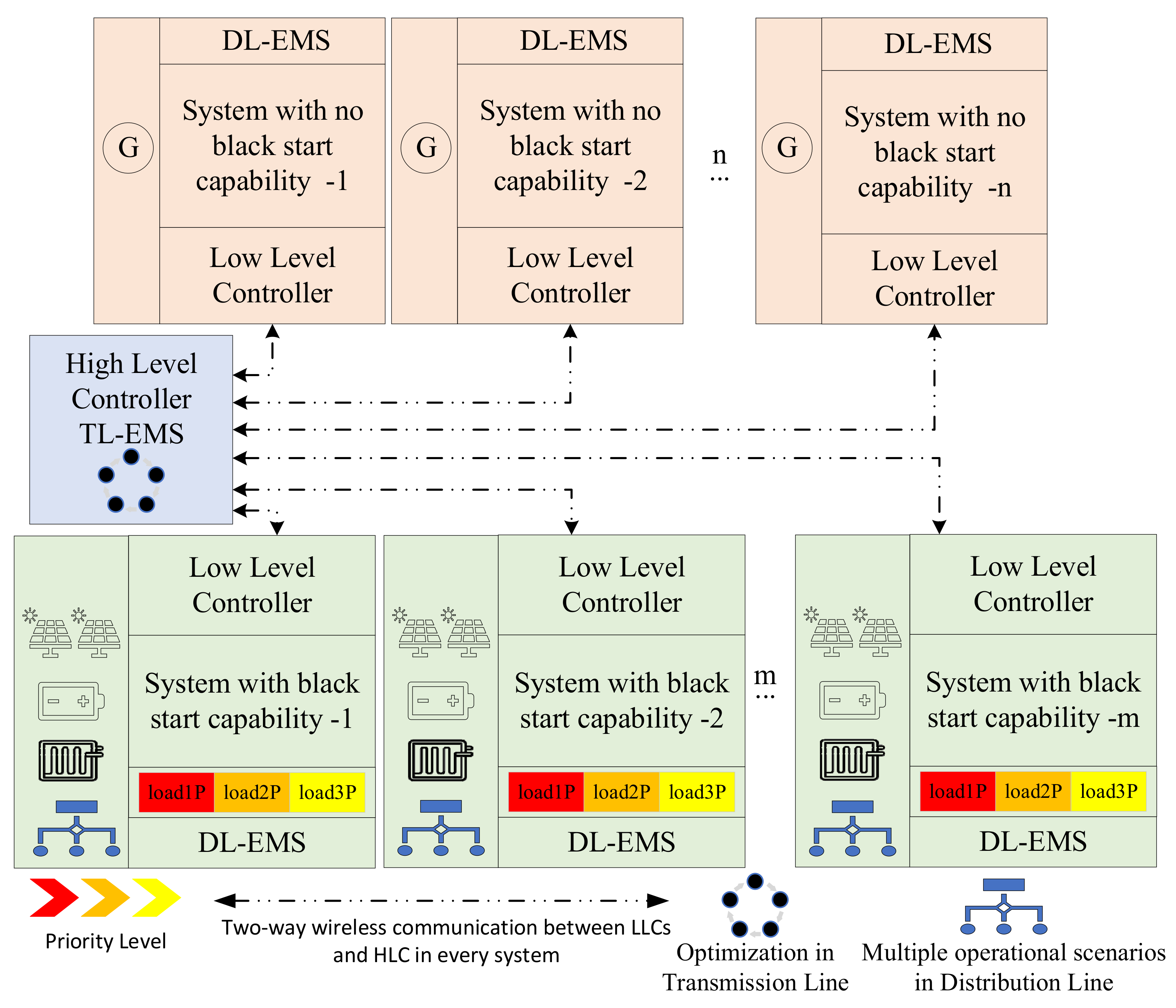
The proposed energy management system employs a multi-level control strategy across the power system. It utilises a hierarchical structure with DL-EMS and TL-EMS to efficiently manage energy within the areas of the power system and maintain overall grid stability, particularly during normal scenarios and emergencies. It categorises areas based on their black start capabilities. Certain areas lack black start capability as they primarily use traditional steam-powered synchronous generators for energy production. These generators require the power grid to be operational in order to start up, limiting their ability to restart the system independently during a blackout. In contrast, areas with black start capability are characterised by their integration of renewable energy sources such as solar panels, batteries, and fuel cells. These distributed renewable energy resources can initiate the restoration of the grid independently, which enhances the overall resilience and sustainability of the power system. The dual layer of the proposed system, including both DL-EMS and TL-EMS under the hierarchical energy management system, significantly enhances operability and coordination. It ensures smooth communication and integrated control across all levels of the energy distribution network, addressing both normal operations and contingency scenarios effectively. The HLC and LLC engage in two-way communication, exchanging various types of information depending on different operational scenarios. Detailed explanations are provided in the following sections. The architecture and operational dynamics of this novel energy management system are depicted in Figure 1.
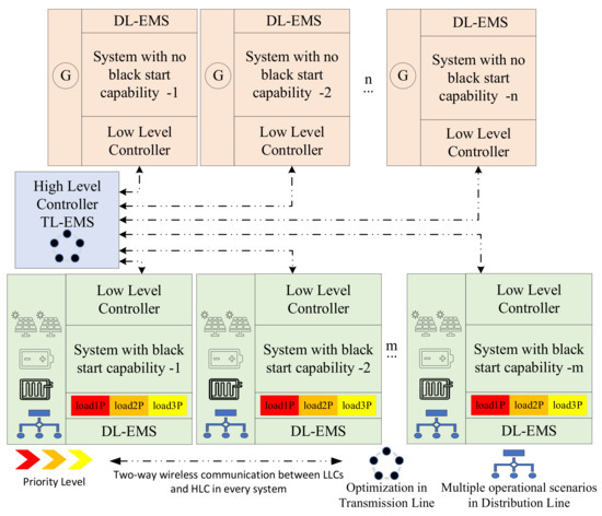
Figure 1.
The proposed hierarchical energy management system including both DL-EMS and TL-EMS.
The network includes ‘n’ DL-EMSs with areas with no black start capability. BSA integrates a hybrid configuration of energy sources, consisting of two parallel-connected solar panels, a battery, and a fuel cell. The use of two parallel-connected solar panels is to demonstrate the proposed management system’s capability to handle parallel solar panel operations. These sources support three different loads to maintain the simplicity of the system while also representing hierarchical order by their criticality, where the first load represents the most critical load and the third load is the least critical one, as shown in Figure 1. A BSA operates under various scenarios including normal operation, black start operation, night operation, load shedding operation, and emergency operation to demonstrate the flexibility and resilience of the DL-EMS managed by the LLC. Conversely, there are m areas with no black start capability (NBSA), which depend on only single conventional steam generators for energy supply to reflect a reliance on traditional power generation. An NBSA operates under only two scenarios, namely, normal operation and black start operation. For simplicity, it is assumed that within this area, all loads are treated uniformly without differentiation based on criticality levels. During blackout scenarios, BSAs initially focus on restoring power to their critical loads. Once stability is achieved and if surplus power is available, these areas then look to support NBSAs in need. It is the role of the TL-EMS to determine the optimal allocation of this excess power from BSAs to NBSAs, ensuring that the distribution is carried out efficiently and effectively. This process takes into consideration the available reserve power within BSAs and the geographical proximity of NBSAs, underlining a novel proposal for power outage management through a hierarchical energy management system. The following subsection describes each area in detail.
2.1. Operational Framework of DL-EMS in Non-Black Start-Capable Areas (NBSAs)
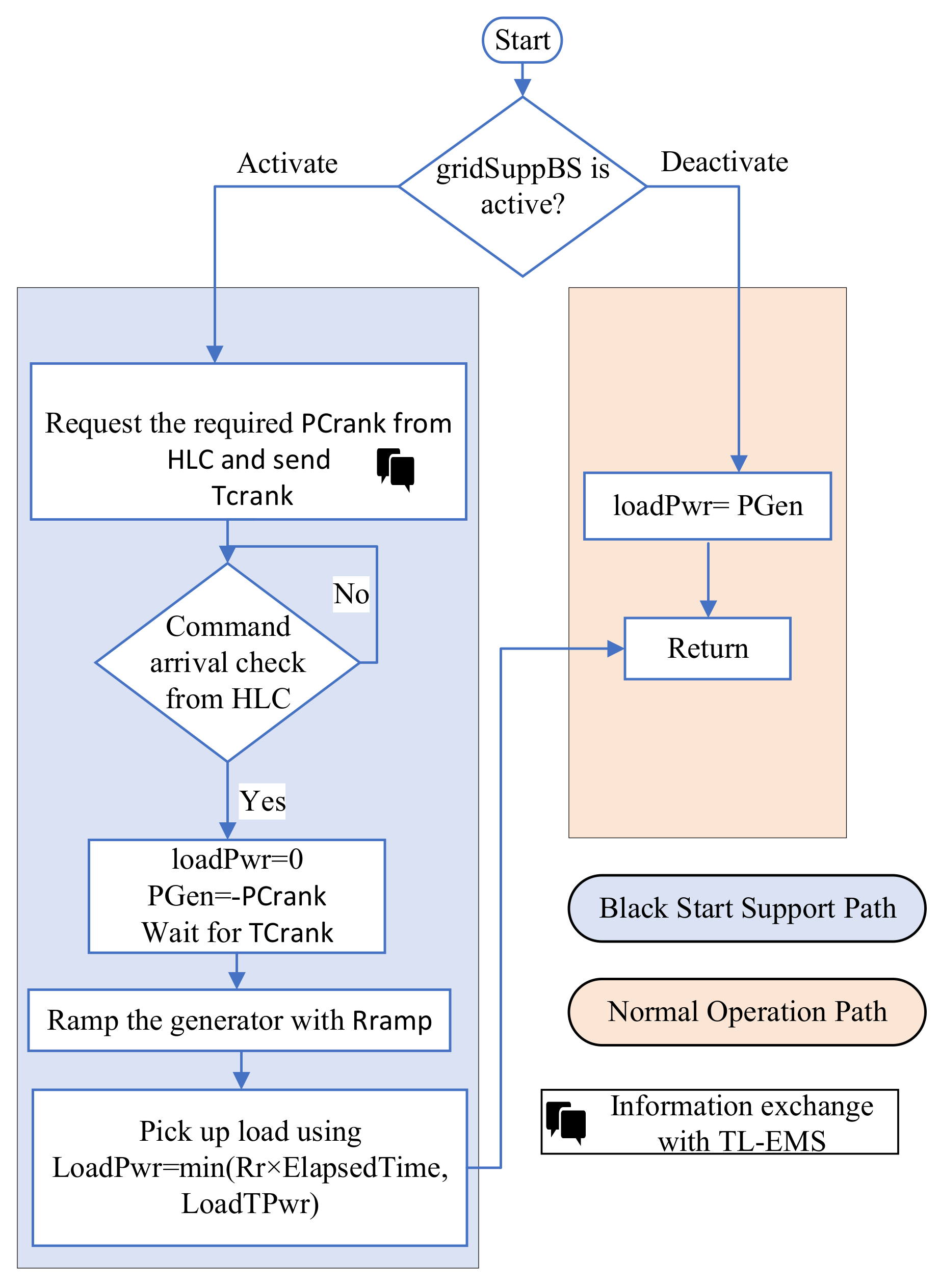
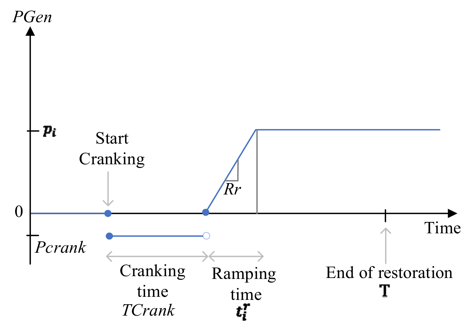
As previously indicated, NBSAs are traditionally equipped with a single synchronous generator for simplicity. There are two primary operational scenarios for these areas, as shown in Figure 2, which are the black start support path and the normal operation path. Under normal operation, the generator power (PGen) is adjusted to meet load demand power (loadPwr) using its governor system to achieve a balance between the load and generation, and system stability is maintained. However, the inherent challenge with synchronous generators is their dependency on an external electricity supply to start up during black start conditions. This necessity is graphically represented in Figure 3, where the generation capability curve indicates that the generator must be supplied with a specific cranking power () for a defined period, known as the cranking time (), to begin starting up. After this period, the generator has the capacity to produce power, but its output increases gradually in accordance with the ramp rate (). Accordingly, loads within the NBSA are incrementally reintroduced to service as the generator progresses along the ramping curve, incrementally generating more power. This sequence continues until all the loads in the area have been reconnected. At this point, the generator is considered to have successfully started up and transitions to the normal operation path. Moreover, the LLC of NBSAs necessitates communication with the HLC at the transmission level. This involves transmitting not only the required power and cranking time but also two critical parameters: the minimum critical time (Tgcmin) and the maximum critical time (Tgcmax). These parameters indicate the timeframe within which the generator must be cranked. If an NBSA does not start within the corresponding maximum critical time, the unit will become unavailable after a considerable time delay. Furthermore, an NBSA with the minimum critical time is not ready to receive cranking power until after this time. Thus, the HLC optimally allocates this cranking power from the nearest BSA within these timeframe constraints. Upon receiving the command about the availability of the cranking power from the HLC, the generator in the NBSA begins to crank and moves to operational status.
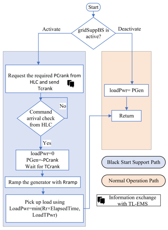
Figure 2.
Flow chart of DL-EMS in non-black start-capable areas (NBSAs).

Figure 3.
Generation capability curve.
2.2. Operational Framework of DL-EMS in Black Start-Capable Areas (BSAs)
The DL-EMS within BSAs is structured to efficiently transition between several operational scenarios. These include normal operation, black start operation, night operation, load shedding operation, and emergency operation. The control strategies for the normal and black start operations are shown in Figure 4, while Figure 5 illustrates the remaining operational scenarios. This study assumes the first load () is the most critical load while the third load () is the least critical load, as shown in Figure 1. Moreover, the DL-EMS within the BSAs demonstrates advanced intelligence by optimising load distribution based on predictive solar energy data for the next day and user preferences. It ensures operational satisfaction by aligning energy management systems with customer-chosen criteria, thereby integrating a customer-centric proposal within the technical framework of power distribution. This proposal reflects the demands of its end-users. Furthermore, forecasting solar irradiance for the next day enables the system to strategically adjust daily load management, thus safeguarding and optimising power availability for next-day operation. The following parts describe the different scenarios in detail.
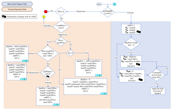
Figure 4.
Flow chart of DL-EMS in black start-capable areas (BSAs): detailing the paths for normal operation and black start support.
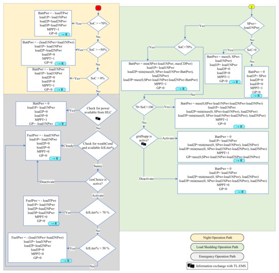
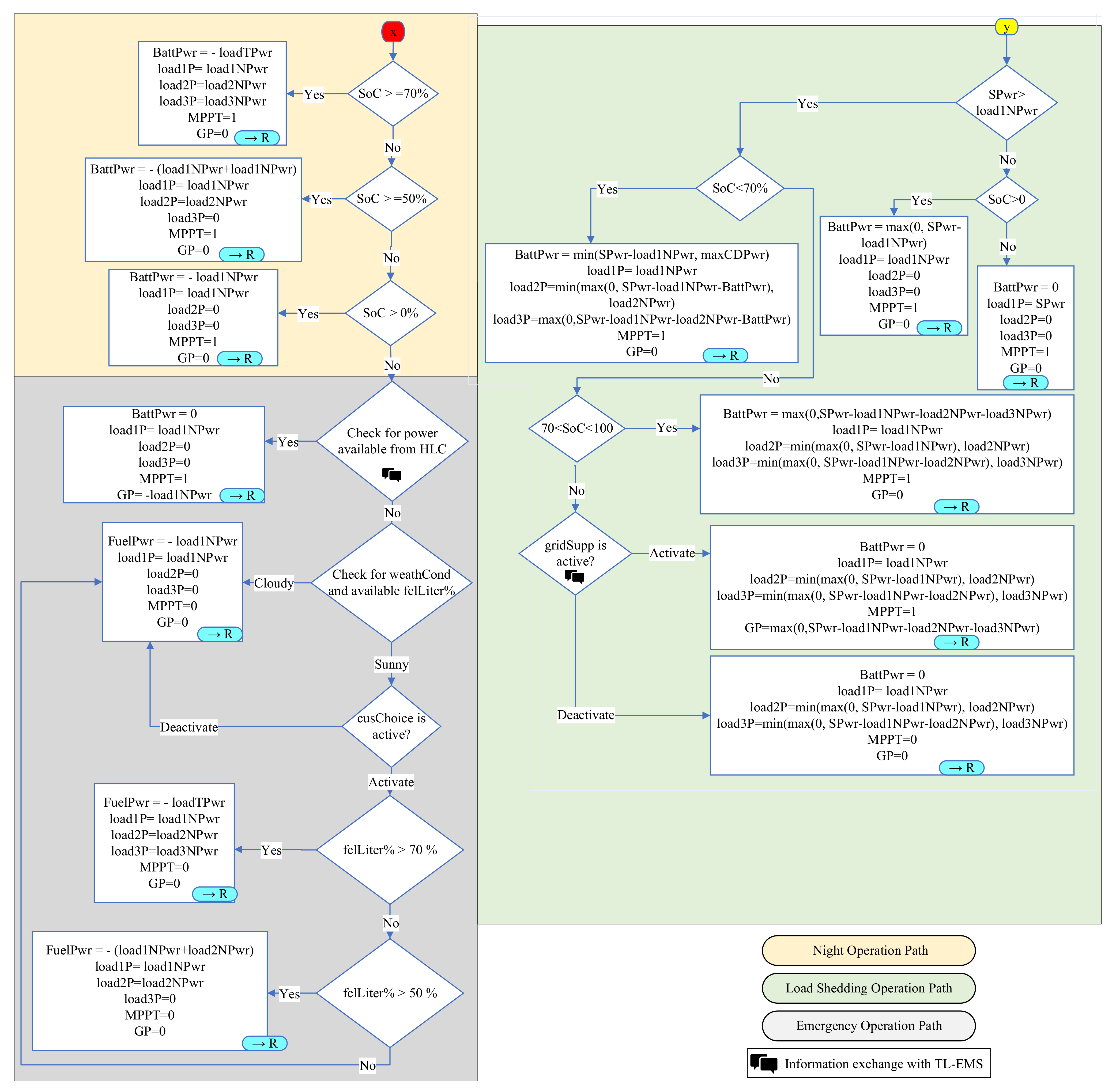
Figure 5.
Flow chart of DL-EMS in black start-capable areas (BSAs): detailing the paths for night operation, load shedding, and emergency operation.
2.2.1. Normal Operation Path
During normal operation, which occurs when solar power (SPwr) is available and load shedding (LoadShed) is deactivated by the user, the controller first assesses whether the available solar power can meet the combined total demand of all the loads (loadTPower) in the system, , , and . If so, these loads are powered to their full nominal power. The controller then evaluates any surplus power. If solar power exceeds demand and if the battery is not fully charged, the surplus is directed towards battery charging without exceeding the battery’s maximum charging capacity. If the surplus exceeds the limit, the controller communicates with the HLC to determine if the excess can be dispatched into the grid. If not, the system is adjusted to operate the solar panels in voltage regulation mode to bypass maximum power point tracking to match the load nominal power (LoadNPwr) and charge the battery within its limits.
If solar power falls short of covering the nominal power for all three loads (Load1NPwr, Load2NPwr, Load3NPwr), the controller checks the battery state of charge (SoC) to decide if combined solar and battery power (BattPwr) can fulfil the nominal demand for the three loads. The battery compensates for the shortfall up to the total nominal demand minus the solar contribution. In scenarios where the battery lacks sufficient power with zero SoC, solar power is allocated based on load priority: is assumed to be the most critical load, followed by and as power availability permits. This prioritisation ensures that the most critical loads are supported first, as shown in Figure 4.
2.2.2. Black Start Operation Path
In black start scenarios, the LLC within the BSA receives a command from the HLC indicating the need to assist neighbouring areas in initiating their startup processes. In response, the LLC maximises solar generation through precise MPPT and sends the current load conditions to the HLC. Therefore, depending on operational feasibility, the LLC provides feedback. If the current load states prevent support, the HLC might request the LLC to shed less critical loads to allocate more power for the black start effort where necessary. Subsequently, the LLC assesses the available reserve power from its array of sources: battery, solar, and fuel cell. It begins by evaluating the battery SoC and its current power status. If the battery is in a charging state, benefitting from surplus solar power, then the reserve power for solar is considered to be the excess energy directed towards unnecessary battery charging. Moreover, the battery reserve power is considered at its maximum discharge capability assuming it has not been fully discharged. Conversely, if the battery power status is discharged, there is no surplus solar power, resulting in the solar reserve being zero. The battery reserve power, in this scenario, is assessed based on its maximum charging capacity minus the power being utilised to compensate for load deficits. If the battery is discharging at or near its maximum capacity to support the loads, its available reserve for black start is zero.
The LLC then sends the calculated reserve powers from the solar array, battery, and fuel cell, alongside the battery SoC and the fuel cell available fuel percentage, to the HLC. This enables the HLC to estimate the duration these reserves can sustainably support the black start operation. Based on this analysis, the HLC solves an optimisation problem, detailed in subsequent sections, to determine the optimal power dispatch strategy. Operational instructions are then sent back to the LLC on how much power is effectively needed from this BSA to support neighbouring areas during the black start process, as shown in Figure 4.
2.2.3. Load Shedding Path
During the load shedding path, priority is assigned to charging the battery rather than supplying power to the least critical loads. This approach differs from normal operations, where the preference is to support all loads before charging the battery, as shown in Figure 5. In this scenario, the LLC evaluates whether solar power can fully supply the most critical load (). If solar power is insufficient, the controller checks the battery SoC. If the battery is charged, both solar and battery power are utilised to supply to its full capacity. However, if the battery is fully discharged, operates below its normal capacity, relying solely on the available solar power.
In the case that solar generation is above the requirements of , the LLC progresses to the next evaluation phase, examining the battery SoC to determine if it exceeds the threshold considered safe for night-time operations, assumed to be 70%. If the surplus power, after supporting , exceeds the battery’s maximum charging capacity, the controller allocates the remaining surplus to supply according to its criticality. Any additional power, after attending to and maximising battery charging, is then directed to . Conversely, if the battery SoC is above the safe threshold, the system shifts its operational focus to powering and , based on their respective criticality levels. If there is excess solar power after supporting these loads, the battery begins to charge with the surplus until it reaches its maximum SoC. Upon reaching this limit and if additional solar power remains, the LLC asks the HLC to determine the need for this extra power in the grid. If external support is not required, the LLC disables the MPPT and switches to voltage regulation mode, distributing the remaining solar power to the three loads as per their criticality. The load shedding operation path is determined based on the estimated irradiance for the day. If the irradiance is projected to be low, the load shedding mechanism is activated.
2.2.4. Night Operation Path
During night-time operation, when solar irradiance is unavailable and solar panels do not contribute power, the system relies entirely on battery reserves to supply the loads, which are prioritised according to their criticality. Specifically, if the battery SoC exceeds 70%, it possesses sufficient energy to simultaneously power all three loads at full capacity. However, in cases where the SoC falls between 50% and 70%, the battery’s reduced capacity necessitates the disconnection of the least critical load () to ensure system stability, allowing only the two more critical loads ( and ) to be powered fully. In scenarios where the SoC is between 10% and 50%, the available battery power is allocated exclusively to the most critical load (), with the less critical loads ( and ) being disconnected from the system. The choice of maintaining a minimum SoC threshold of 10%, rather than discharging the battery entirely to 0%, is made to avoid full discharge, thereby extending the battery lifespan. In cases where the SoC drops below 10% without the availability of solar power, the system moves to an emergency operation mode, as shown in Figure 5, to manage the remaining energy resources effectively.
2.2.5. Emergency Operation Path
In the scenario where the DL-EMS within the BSA faces an emergency situation due to insufficient solar and battery resources to power the critical loads, the EMS asks for power from the HLC. The LLC inquires if available power can be supplied from adjacent areas through the grid to feed the most critical load (). If the HLC manages to secure the required power, it is directed to support . However, if the HLC is unable to obtain external power for , the system then relies on its fuel cell as a backup energy source. The allocation of power from the fuel cell is prioritised based on load criticality and the available fuel percentage. Utilising its intelligent capabilities, the DL-EMS forecasts the next day’s solar irradiance. If a cloudy day is expected and there is sufficient fuel, the system prioritises conserving fuel by supplying power only to , preparing for limited solar generation for the next day. Conversely, if sunny conditions are expected, reducing the need to conserve fuel, the LLC consults with the customer to determine their preference regarding the distribution of power among the loads (. This step enhances user satisfaction by allowing choices in power distribution based on available resources. In case the customer chooses to support all loads and the fuel cell capacity is above 70%, the system can power all loads fully. If the fuel capacity is between 50% and 70%, the system will power only the first two critical loads. However, if fuel levels drop below 50%, the decision is made to supply power solely to the most critical load. This approach not only incorporates intelligent system management and customer input into operational decisions but also ensures effective integration with the grid power (GP) supply capabilities.
2.3. Operational Framework of TL-EMS for High-Level Controller (HLC)
For the TL-EMS centralised under the HLC that interlinks all the LLCs from various areas, the HLC is pivotal in coordinating between them. It primarily functions in two scenarios: normal operations and black start operations. During normal operations, the HLC’s role is to optimally manage power distribution, especially in emergency scenarios where a BSA requires additional power. In case a BSA needs supplementary power for its critical loads, the HLC surveys both BSAs and NBSAs for any available surplus power. If found, the HLC efficiently determines and dispatches the optimal allocation of this excess power to the BSA in need. Conversely, if no additional power is available from surrounding areas to support the BSA during its emergency, the HLC communicates back to the BSA, as illustrated in Figure 6.
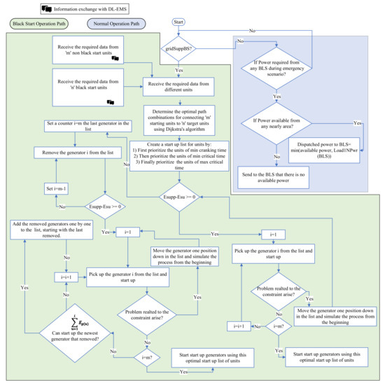
Figure 6.
Flow chart of TL-EMS for the centralised HLC.
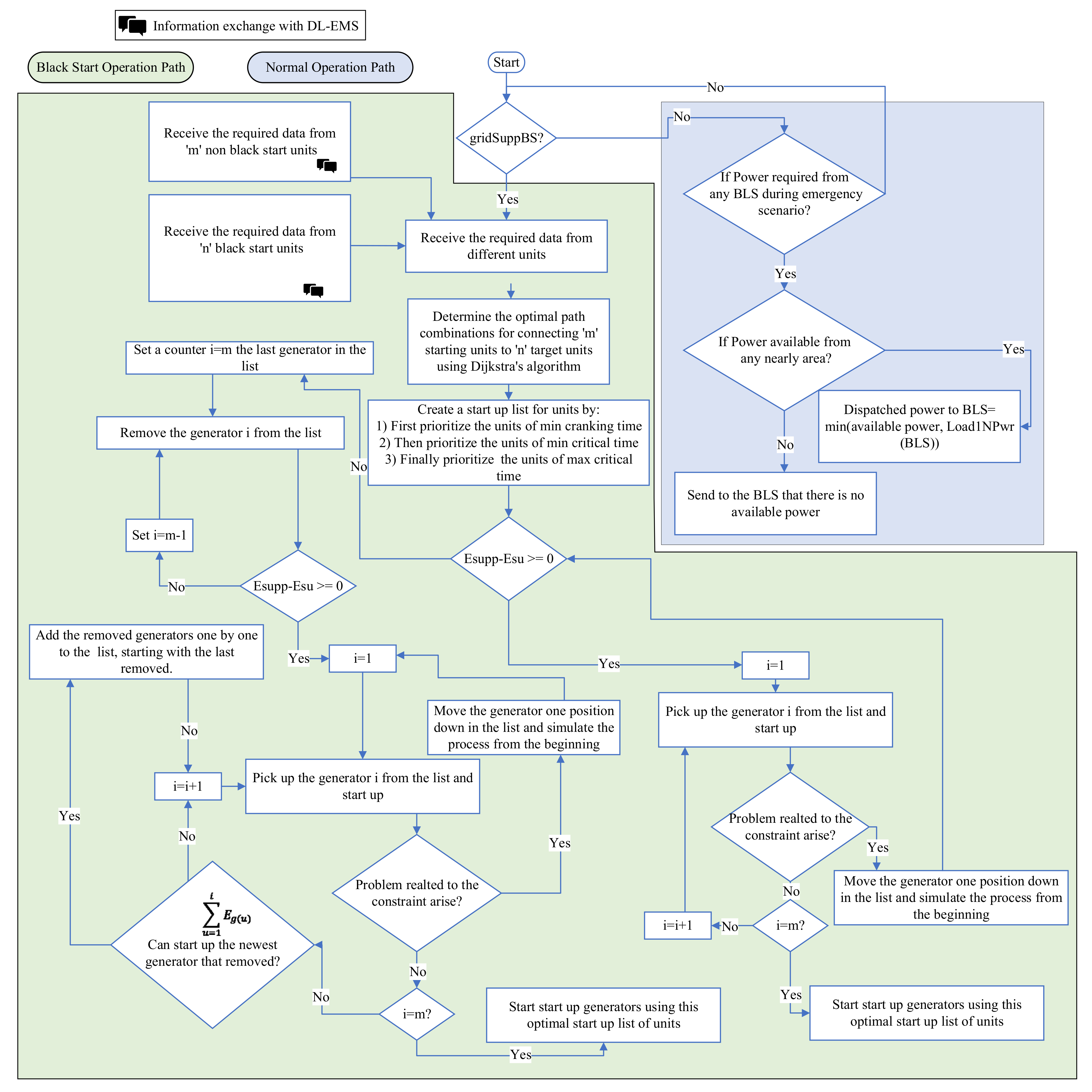
In black start scenarios, the HLC requests essential information from both the BSA and NBSA. From the BSA, the HLC gathers data on available reserve power sources, including solar, battery, and fuel cell, along with the status of less critical loads such as and . This information is crucial because, in situations where available power is insufficient, the HLC may decide to disconnect these lower-priority loads to conserve power for black start operations, albeit as a last option. Additionally, the HLC collects details on battery capacity, SoC, fuel capacity, fuel level, and estimated solar availability from the LLC intelligent forecasts. This comprehensive dataset aids the HLC in determining how long these resources can sustain the black start process to prioritise the resources that can reliably support operations until successful completion. From the NBSA, the HLC receives information about the cranking power needed for each generator, including cranking times and generator characteristics such as minimum and maximum critical times.
The HLC ensures that power supplying occurs within these critical timeframes to guarantee successful startup. Upon compiling this information, the HLC employs Dijkstra’s algorithm to identify the optimal routing for connecting BSA and NBSA buses. This algorithm considers network resistance to minimise total path losses during the black start to optimise energy distribution. The HLC then constructs a preliminary generator startup sequence, ranking generators based on their readiness and critical timing constraints. Generators with shorter cranking times are prioritised and are followed by those with urgent critical timing needs. If generators have similar cranking times, then preference is given to those with narrower windows between their minimum and maximum critical times to ensure no generator startup falls outside its critical window. Finally, the HLC calculates the energy reserves from the BSA and compares it with the energy demanded by the generators to start up in the NBSA using the following equations:
where and are the total reserved energy from the BSA and the total energy required by the generator to start up, respectively. is the reserved power from solar energy, is the reserved power from the battery, is the reserved power from fuel cells, is the estimated time of irradiance lasting in hours, is the total capacity of the battery, is the percentage of fuel in the tank, is the total capacity of the tank in litres, is the energy density of the fuel (kWh per litre), and is the efficiency of the fuel generator.
In cases where energy reserves from the BSA exceed the demand of NBSA generators, the HLC sequentially addresses each generator to refine the startup list based on operational constraints. If a generator encounters optimisation issues, adjustments are made to the sequence to address any conflicts to ensure a smooth startup process for all generators. For example, if the scheduled startup time for a generator on the list falls before its minimum critical time, that generator is moved up one position in the sequence. Conversely, if a generator startup time exceeds its maximum critical time, it is shifted one position down in the list.
On the other hand, if BSA reserves are inadequate for all NBSA generators, the HLC removes some generators in the list from the bottom up to focus on generators with less strict operational constraints. This iterative process continues, then the HLC reintegrates generators in the list as more energy becomes available from already activated generators, always prioritising reintegrating those with stricter operational necessities. Ultimately, this detailed procedure ends in a refined, optimal startup sequence list. Following this optimised list, the HLC coordinates the startup of NBSA generators. This strategic approach guarantees that following the refined startup sequence will lead to the error-free activation of all targeted generators, effectively restoring power without issues. The subsequent part outlines the optimisation problem and constraints employed by the HLC in formulating the optimal startup sequence for generators.
3. Objective Function of the Optimisation Problem
This section presents a mathematical model for the TL-EMS operated by the HLC, aimed at improving grid restoration following a blackout. The model includes three objectives: enhancing system inertia to stabilise the grid during black starts, refining load shedding to ensure critical loads are maintained, and expanding the renewable energy use in grid restoration. The heart of this system is a novel multi-objective optimisation function, combining the following objectives: for system inertia, for load prioritisation, and for renewable integration into a unified goal to enhance overall performance. This optimisation framework is defined as follows:
In this model, represents the objective to enhance the grid inertia by optimising the allocation of reserve power, mitigating frequency deviations. focuses on minimising power supply to non-essential loads, thereby ensuring priority is given to critical services during the restoration phase. emphasises increasing the grid’s reliance on renewable energy, integrating sustainable solutions into the black start process. Each objective is defined by specific equations that illustrate their individual contributions to the grid recovery strategy. For instance, is described as follows:
In this model, the distribution factor () for each area is determined based on the outcomes of Dijkstra’s algorithm, which identifies the optimal paths between BSAs and the generators in NBSAs planned for startup. The model assigns weights to these paths, favouring shorter routes with higher values over longer ones. Consequently, the distribution factor enhances the prioritisation of areas closer to the generators being activated, ensuring they receive power more promptly, which contributes to greater grid stability and reduced transmission losses. is the reserve power from source in area . Furthermore, the term represents the estimated duration for which power sources like solar, fuel cells, and batteries can sustain their output, informed by the LLC predictions on solar availability and the current SoC and fuel level percentage. denotes the response time for source in area ; it reflects how quickly a power source can react to disturbances. Therefore, the inertia contribution increases as the reserve power and its availability duration increase and also increases as the source’s response time shortens. Finally, the model combines the objectives of minimising unnecessary load shedding and enhancing the integration of renewable energy using Equation (5). This dual objective is captured in a unified minimisation function as follows:
where is a vector that symbolises the collective available reserve power from diverse sources such as solar energy, batteries, and fuel cells.
The objective function also categorises loads into two categories, less critical and least critical, to optimise power distribution with the application of binary variables (). This approach ensures customised energy allocation, focusing on the prioritisation of power delivery based on load criticality. For example, disconnects the least critical loads and introduces its power in the black start operation in case the reserving power is not sufficient. disconnects the less critical loads and introduces its power in the black start operation in case the reserving power and least critical power are not sufficient. Furthermore, the model introduces penalties ( and ) to discourage the unnecessary shedding of loads and to promote the integration of renewable energy. and are large positive numbers with being substantially larger than . Moreover, the optimisation function in (5) incorporates functions ( and ) designed to account for the power source location and cost. Specifically, (i) the distance-based penalty function applies penalties for using power sources based on their distance to the NBS area and the type of source. This encourages the use of closer and more cost-effective energy sources.
where is the distribution factor related to the proximity to the NBSA. is a penalty coefficient and varies based on the type of power source, with a preference for those that are less costly (e.g., solar panels are preferred over batteries, and batteries over fuel cells), ensuring an efficient and cost-effective power restoration process. (ii) The load shedding cost functions and evaluate the financial impact of disconnecting non-critical and priority loads, respectively, aiming to minimise these actions unless absolutely necessary.
Constraints of the Optimisation Problem
The optimisation model integrates various constraints essential for maintaining grid stability and operational efficiency. These constrains can be summarised as follows:
- Distribution factor constraint:
This ensures that the sum of distribution factors in (4) and (5) across all areas equals 1 . This constraint plays a pivotal role in determining the allocation of power based on the geographical proximity of areas to the black start zone by using Dijkstra’s algorithm. Areas closer to the black start area are assigned higher distribution factors, reflecting their increased importance in power distribution.
- 2.
- Power balance constraint:
The power balance constraint is another critical component, formulated to ensure that the total power generated, including adjustments for non-critical and priority loads, matches the requirements for the black start operation ( of the chosen generator. This balance is vital for upholding system stability.
- 3.
- Voltage and power transmission constraints:
This constraint regulates the voltage levels and power flow within the grid to ensure that the voltage at any bus remains within predefined limits and that the power transmitted along any line does not exceed its capacity. These constraints prevent potential overloads and contribute to the reliable operation of the grid during restoration.
where represents the voltage level at bus and B is the total number of buses. and represent the active and reactive power flow, respectively, between buses and . denotes the voltage level between these buses at the specified time, and is the apparent power limit of the line connecting them.
- 4.
- Operational characteristics and capacities:
Furthermore, the model includes specific operational characteristics and capacities of energy storage and generation units, including batteries and fuel cells. Constraints related to these units ensure their output aligns with operational capabilities and state of charge, securing against overutilisation.
These constraints ensure that if batteries and fuel cells are selected to support the black start process, they will be capable of providing continuous support throughout the entire cranking period, thereby enhancing the system stability during black start operations. represents the power output from the battery storage in area , denotes the time for the cranking of non-black start units, is the state of charge of the battery in area , and is the capacity of the battery in that area. Moreover, is the power output from the fuel cells in area , and is the available capacity. Additionally, if the solar panel in area is selected to power the black start, it must be verified that the power can be sustained throughout the entire cranking period. This is achieved by ensuring that the cranking time does not exceed the duration of sunlight availability, as predicted by the LLC of area .
- 5.
- Operational Timing Constraints for Generator Startup
These constraints are pivotal in ensuring successful startup of both generators without black start capability such as steam turbines. For instance, operational timing constraints are formulated as follows:
These constraints ensure that NBSAs’ start operations are performed within a specific timeframe: the start time () must not exceed the critical maximum time interval (), ensuring readiness for activation before becoming critical to the restoration process. Conversely, () should not precede the critical minimum time interval (), allowing for preparations that ensure a stable startup. These timing constraints are essential for the orderly and efficient re-energisation of NBSA generators, facilitating a coordinated restoration process.
4. Results and Discussion
In this section, two different experiments are conducted and their results are discussed. Firstly, the functionality of a DL-EMS within a BSA is assessed via MATLAB/SIMULINK simulations, validating its performance across various scenarios including normal operation, black start, night-time operation, load shedding, and emergency situations. Secondly, the black start scenario is examined within the framework of the TL-EMS under the HLC, aiming to assess the efficiency of transmission line control strategies and the black start scenario’s performance of the DL-EMS within the BSA.
4.1. DL-EMS in a BSA
The performance of a DL-EMS in a BSA is evaluated through a MATLAB/SIMULINK simulation. The specified BSA configuration includes a pair of solar panels operating in parallel, coupled with a battery storage unit and a fuel cell system, all of which are interfaced with the local utility grid. This comprehensive validation includes various operational scenarios, namely, normal, black start, night, load shedding, and emergency operations. Figure 7a,b show outcomes associated with the normal operational scenario wherein load shedding is inactive.
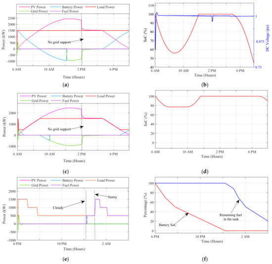
Figure 7.
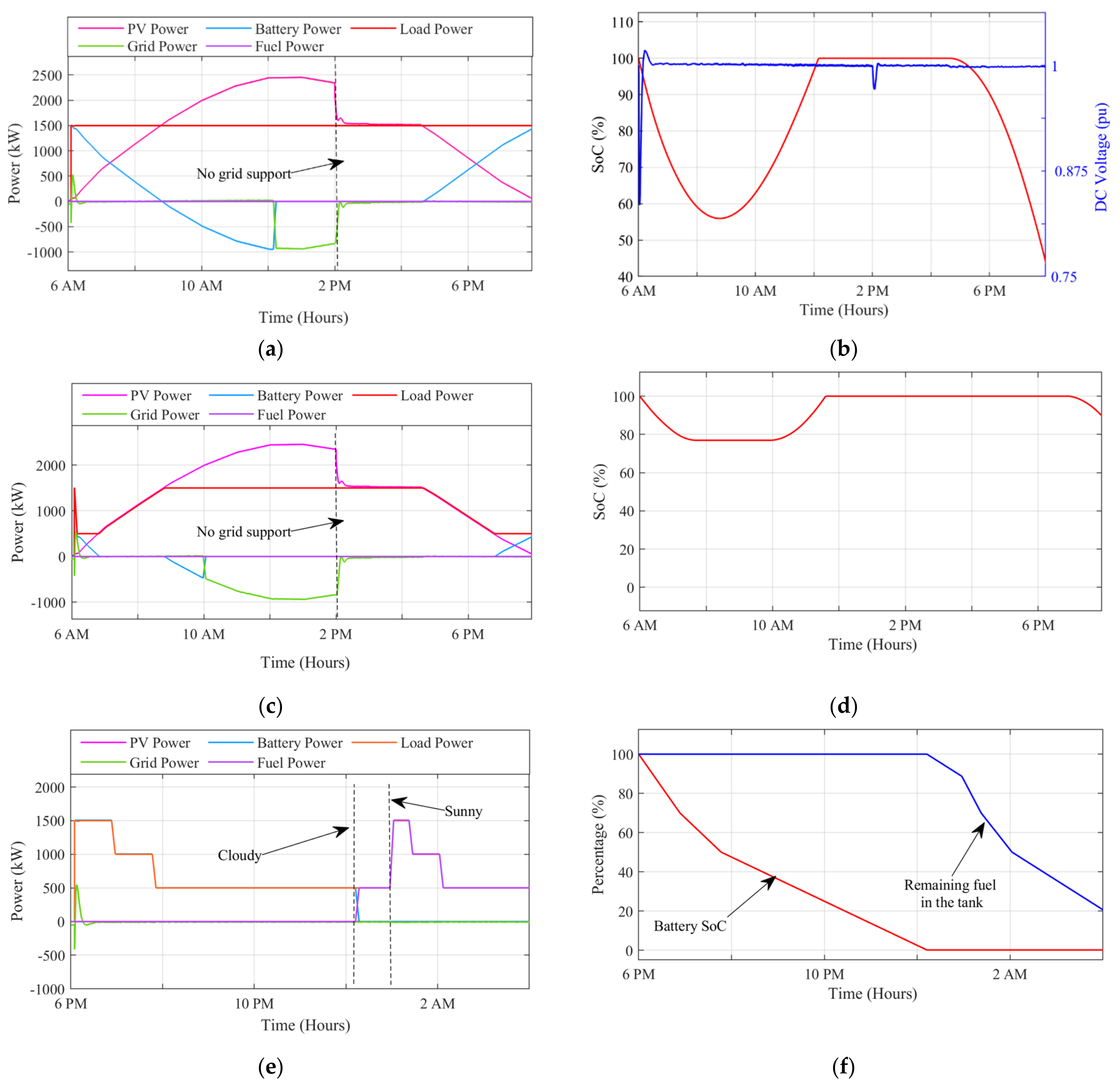
(a) Daily power flow in the normal scenario: solar, battery, BSA load, fuel cell power, and grid interaction power. (b) Normal scenario battery SoC and DC voltage of the PV side throughout the day. (c) Daily power flow in load shedding scenario: solar, battery, BSA load, fuel cell power, and grid interaction power. (d) Load shedding scenario battery SoC throughout the day. (e) Daily power flow in night and emergency scenarios: solar, battery, BSA load, fuel cell power, and grid interaction power. (f) Night and emergency scenario battery SoC and remaining fuel percentage in the fuel tank throughout the day.
Within this mode, priority is accorded to the operation of all loads in the presence of solar irradiation. As shown in Figure 7a, the power generated by the solar panels follows the expected pattern of increasing with sunrise, peaking at midday, and decreasing towards sunset. Initially, when solar power is not enough to meet the total demand, the system uses both solar and battery power to cover all loads until about 9 AM. By midday, the solar power is sufficient for both load demands and to charge the battery. After the battery is fully charged, which is evident by the 100% SoC shown in Figure 7b, any additional power is then supplied to the grid, which happens just after 12 PM.
At around 2 PM, when the HLC indicates that extra power is not needed, the system stops supplying power to the grid, and the grid support (gridSupp) in the DL-EMS is deactivated. The DL-EMS then switches off the MPPT and changes to voltage regulation control for the solar panels, adjusting their output to just meet the requirements of the three loads. This operation continues in voltage regulation mode until about 5 PM. After this, as the solar output drops below the total load demand, the battery starts discharging to ensure all loads continue to receive power. During this process, the system keeps the DC voltage stable, as shown in Figure 7b. Throughout this, there is no need for fuel cell power (FPwr), as the scenario does not include any emergencies, and the system focuses on powering all three loads continuously. Figure 7c,d illustrate the load shedding operational scenario for the DL-EMS.
Under this scenario, the system operates primarily on solar power, with load shedding actively involved. According to the predetermined operational pathway, priority is given to charging the battery before supporting the two less critical loads, as long as the battery’s SoC is below 70%. Initially, when solar power alone is insufficient for the most critical load, the battery supplements the shortfall. As the morning progresses and solar power generation exceeds the demand of the critical load, battery charging does not take priority, as the SoC is already above 70%, as demonstrated in Figure 7d. In such cases, the additional solar power is distributed to the loads, with the less critical load receiving power based on the available solar energy. It is important to note that the battery does not discharge to support the less critical loads beyond its nominal power during this period. This strategy preserves battery reserves for night-time operation. By 9 AM, when solar production surpasses the combined demand of all three loads, any surplus energy contributes to battery charging until it reaches full capacity. Thereafter, any excess is sent to the grid. This sequence continues until approximately 3 PM when the need for excess power in adjacent areas ceases, prompting the deactivation of grid support. The system then switches to voltage regulation mode, similar to the normal operational strategy. Approaching 5 PM, as solar power reduces below the total load demand, the system adapts by allocating the available solar power to the less critical loads (Loads 2 and 3) without relying on the battery. In keeping with the load shedding protocol, the system progressively reduces power to these non-critical loads as solar input decreases. Finally, by 7 PM, when solar energy falls short of even the most critical load’s demand, the battery intervenes to sustain full operation of this critical load.
In scenarios where solar power is not available, the system transitions to its night operation mode. Figure 7e,f describe the night operation and emergency scenarios. With the battery initially fully charged at 100% SoC, it begins to supply energy to all connected loads. As the battery’s charge level reduces, it progressively reduces support, disconnecting power to Load 3 at approximately 7 PM and Load 2 by 9 PM, as shown in Figure 7e. In cases where the battery’s charge falls below 10% by midnight, the system enters an emergency operation mode.
At this point, if the weather forecast for the following day indicates cloudiness, the system prioritises power supply to only the most critical load starting from midnight. Conversely, if a sunny day is predicted, the system activates the fuel cell to power all loads starting around 1 AM. This approach ensures that the energy management strategies are tailored to meet user preferences, embodying a user-focused design in the power distribution framework. Moreover, by incorporating next-day solar irradiance forecasts, the system can make informed decisions on load management, thereby enhancing the reliability and efficiency of power provision for upcoming operations. Figure 8 illustrates the grid topology utilised for testing the proposed energy management system. Specifically, Figure 8a depicts the IEEE 39 standard bus system, which serves as the testing environment for the TL-EMS. Conversely, Figure 8b represents the distribution network used to evaluate the DL-EMS.
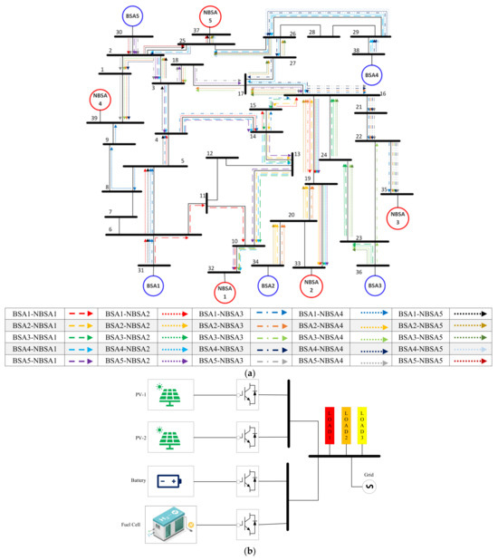
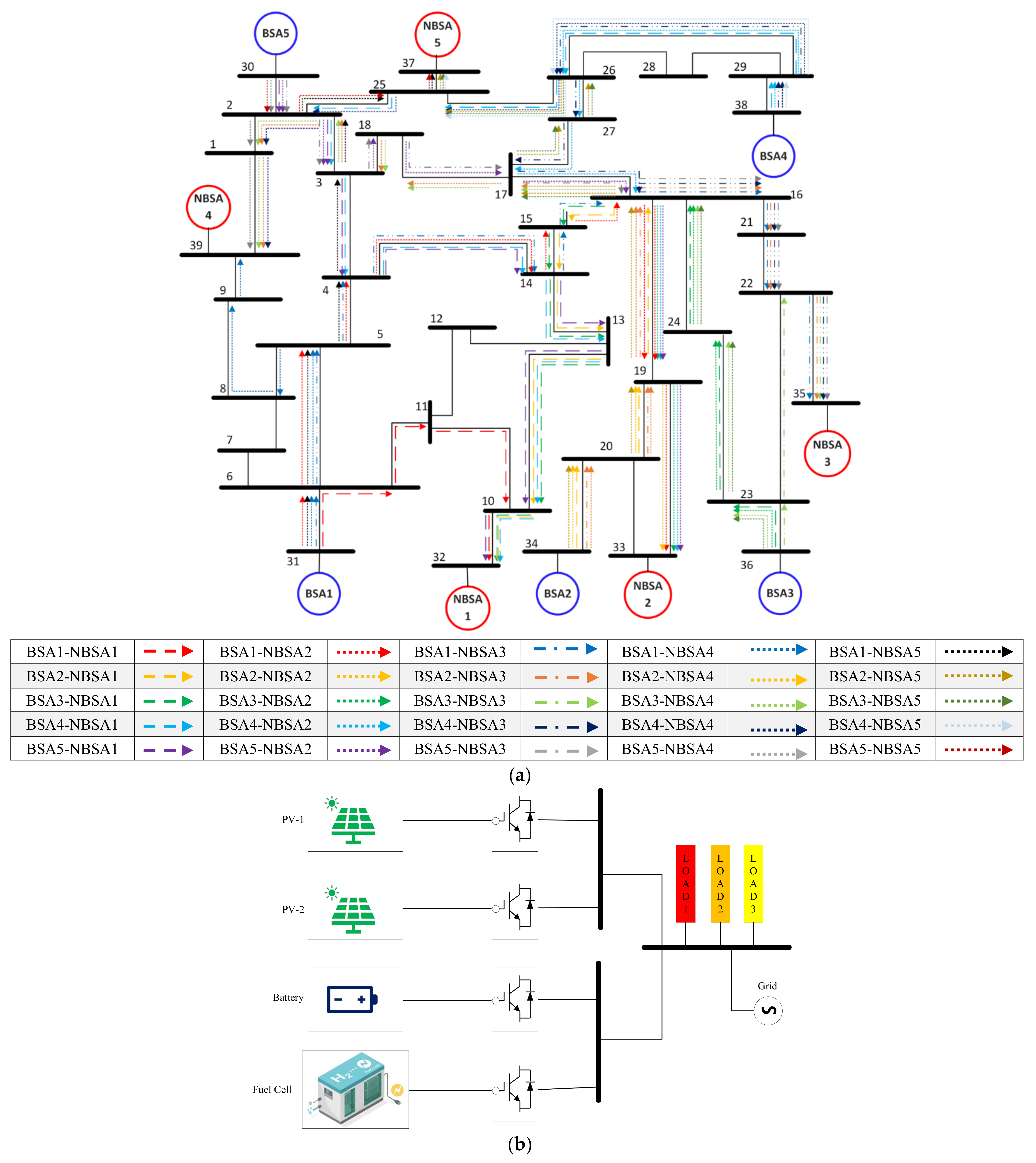
Figure 8.
Comprehensive diagrams of transmission and distribution networks: (a) detailed diagram of the IEEE 39-Bus transmission system with optimal path determination for black start restoration using Dijkstra’s algorithm between BSAs and NBSAs, and (b) detailed diagram of the distribution network for the BSAs.
4.2. TL-EMS under the HLC
The black start scenario is analysed within the context of the TL-EMS under the HLC, to evaluate the effectiveness of the transmission line control strategies and the black start scenario at DL-EMS in BSAs. This validation utilises the IEEE 39-Bus system, segmenting it into ten different areas comprising five BSAs and five NBSAs. The BSAs are situated at buses 30, 38, 31, 34, and 36, while the NBSAs, which include steam generators, are located at buses 37, 39, 32, 33, and 35. In the event of a black start, the HLC within TL-EMS collects data from both BSAs and NBSAs and then identifies the most efficient path from each BSA to each NBSA, as depicted in Figure 8a. The algorithm prioritises the impedance of the transmission lines, applying it as a penalty factor to determine the optimal path, ensuring that the selected path not only is the shortest but also minimises impedance across the network. Table 2 presents the characteristics of the generators situated in the NBSAs, detailing key operational parameters necessary for the black start process. The table lists each generator’s cranking time (), the minimum critical time (), and the maximum critical time (). It also includes the ramp rate (), which is the rate at which the generator can increase its power output per hour, the cranking power () required for initiating the generator, and the generator’s maximum power output capacity (). Moreover, Table 3 outlines the durations necessary to complete various generic restoration actions critical to providing power to NBSAs. It specifies the time required to energise a busbar from a BSU, a busbar, or a line. Furthermore, the duration for synchronisation activities is between busbars or lines. Additionally, the time needed to pick up a load and integrate it into the power system is also documented. These timings are essential for the precise sequencing and coordination of restoration tasks following a blackout.
Table 2.
Data of generator characteristics [15].
Table 3.
Time to complete restorative actions [24].
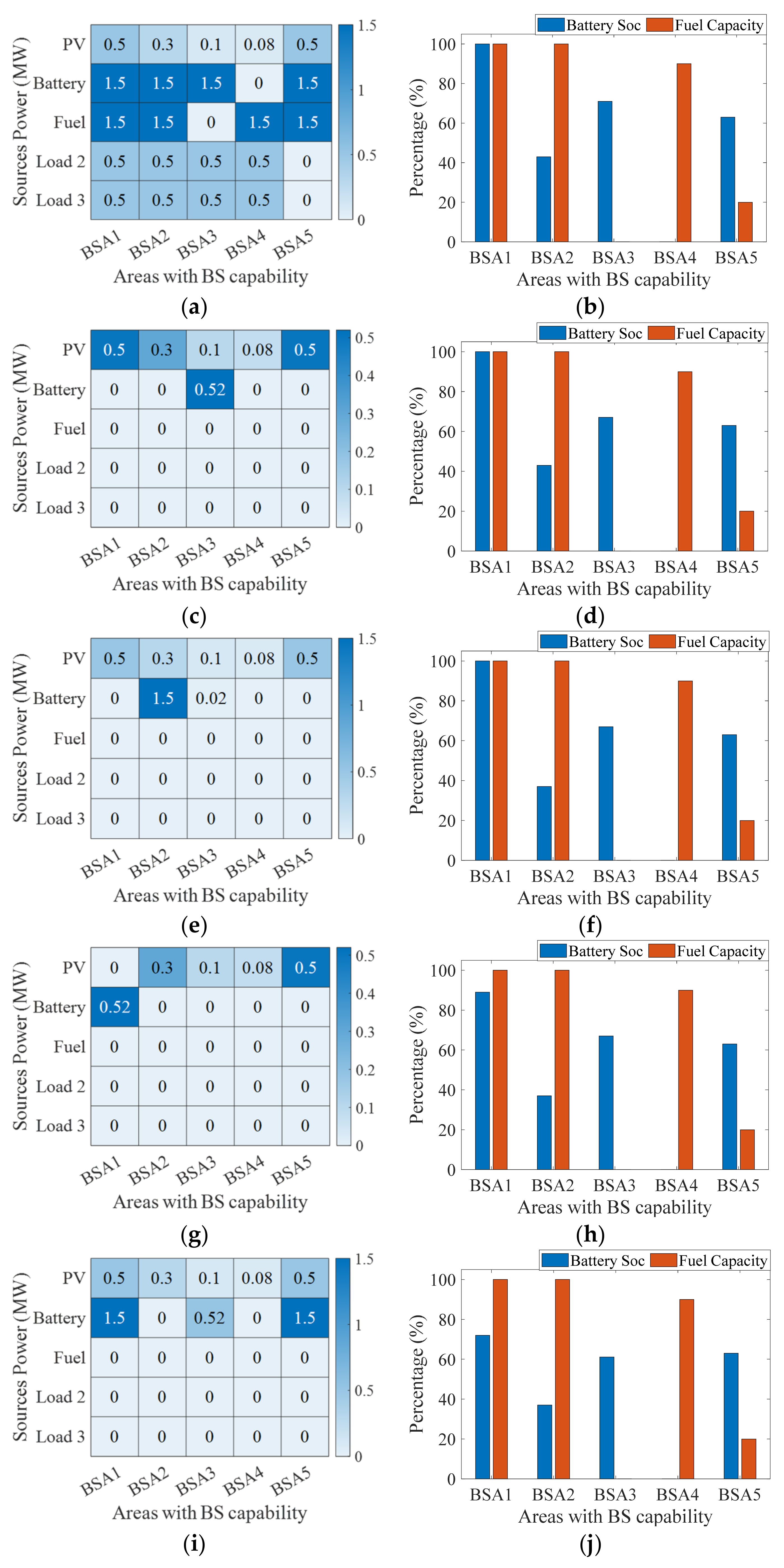
The HLC started the black start process at 10 AM with areas BSA1, BSA3, and BSA5 being assumed to operate under the load shedding scenario, while BSA2 and BSA4 maintained normal operation. The HLC received critical data from these areas, including the reserve power available from solar panels, batteries, and fuel cells, along with the operational status of less critical loads: and . In the event of insufficient power from the primary sources for the black start requirements, the HLC could deactivate these less critical loads, repurposing their power to support the black start. The SoC of the batteries and the fuel percentage for each BSA were also transmitted to the HLC, providing a comprehensive overview of available energy reserves for decision-making. Figure 9a depicts the reserve powers from the various sources against the BSAs, complete with an indication of the operational states of and . As shown in Figure 9a, the reserve power from PV sources exhibits variation across the BSAs, attributed to the differing levels of solar irradiance each area receives. In area 4, the battery has a zero SoC, indicating it is unable to contribute to black start process. Additionally, area 3’s fuel reserves are zero, leaving it non-contributory in the black start process.
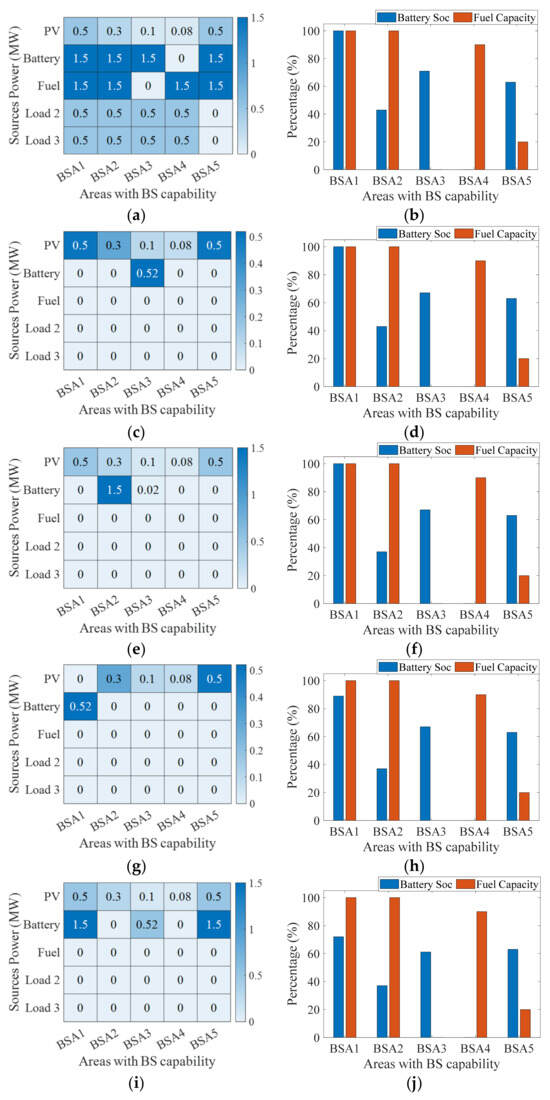
Figure 9.
Information received from BSAs: (a) reserve power distribution and load status in BSAs; (b) battery SoC and remaining fuel percentage in BSAs; (c) optimal power allocation for G3 startup from BSAs; (d) SoC and fuel percentage post-cranking for G3; (e) optimal power allocation for G4 and G2 startup from BSAs; (f) SoC and fuel percentage post-cranking for G4 and G2; (g) optimal power allocation for G1 startup from BSAs; (h) SoC and fuel percentage post-cranking for G1; (i) optimal power allocation for G5 startup from BSAs; (j) SoC and fuel percentage post-cranking for G5.
Finally, the HLC has the option to utilise the power designated for Load 2 and Load 3 across all BSAs, with the exception of BSA5. In BSA5, these loads are not currently powered and are in an offline state. Figure 9b describes the SoC and the available fuel percentages across all the BSAs. From Figure 9, one can observe the varying assumptions across all BSAs, allowing for the evaluation of the proposed EMS under various random operational scenarios and states. Additionally, the HLC gathers data concerning the generators in NBSAs, as well as information about the power network, as detailed in Table 2 and Table 3. Upon receiving the necessary details from both the BSAs and the NBSAs, the HLC proceeds to determine the most efficient order for initiating the generators.
The HLC arranges the generators listed in Table 2 based on their starting characteristics, prioritising those with shorter cranking times. Next, generators with the lowest maximum starting time are sequenced, followed by those with the minimum starting time at the forefront of the list. The final organised sequence for generator startup is G3, followed by G4, G2, G1, and lastly G5. Once the optimal startup sequence is established, the HLC verifies the availability of sufficient reserve energy to cover the energy required from the startup of these generators, by employing Equations (1) and (2). Following a successful assessment of the available reserve energy, the HLC initiates the startup process. This optimisation procedure lasts approximately 5 min, as detailed in Table 4, which outlines the steps to restore the power system. The HLC begins the process of energising each bus and its connected branches, prioritising proximity to the nearest BSA while ensuring the reactive power remains within the capabilities of the BSA.
Table 4.
Actions to restore entire power system.
This energisation occurs simultaneously at various network locations. Starting with BSA3, it powers buses 36, 23, 22, and 25, along with their interconnecting branches as detailed in Table 4. Concurrently, BSA2 activates buses 34, 20, 19, 16, 21, 24, and 33 and their connecting branches. In parallel, BSA4 is responsible for energising buses 38, 29, 26, 27, 17, and 28 and the branches linking them. BSA5 simultaneously energises buses 30, 2, 3, 18, 1, 25, 37, and 39 and their branches. Meanwhile, BSA1 activates buses 31, 6, 5, 4, 14, 15, 7, 8, 9, 11, 12, and 10 and their connections. An attempt is made to also energise buses 13 and 32 from BSA1, but high reactive power could lead to instability in BSA1 operations, postponing their energisation until other buses are powered. This entire process takes about 5 min, as indicated in Table 3 and Table 4.
After powering up most of the buses and linking them to their nearest BSA, the network is divided into several segments without interconnections. The next step involves synchronising these segments to unify the network. BSA3 synchronises with BSA2, while attempts are also made to synchronise BSA4 and BSA5 with BSA1 at the same time. This process, lasting about 10 min as indicated in Table 3 and Table 4, effectively creates two main interconnected zones: one consisting of BSA3 and BSA2, and another comprising BSA1, BSA4, and BSA5. Subsequently, the focus shifts to energising previously postponed buses 13 and 32 within the area that includes BSA1, along with their branches. This energisation takes about 5 min. Finally, the ultimate goal is to merge these two interconnected zones into a single, unified network, a task that also requires around 10 min for synchronisation. Once the network becomes fully interconnected, incorporating all five BSAs, the remaining extra branches that connect buses 18 to 17, 17 to 16, and 15 to 16 are energised, thus fully integrating all areas. With the network now operating as a single interconnected entity, the process moves on to start the NBSAs and integrate them into the grid, completing the restoration effort. The HLC initiates the startup process with G3, identified as the first in the optimal startup sequence. Figure 9c illustrates the optimal power allocation determined by the HLC’s optimisation problem, using available BSAs to supply the necessary cranking power to G3. Predominantly, the power for G3 originates from BSA3, the closest BSA to G3, with solar PV energy prioritised due to its lower cost, making it the preferred energy source from all BSAs. The only battery power utilised comes from BSA3, offering the most efficient cranking solution for G3. Figure 9d shows the subsequent changes in the SoC and fuel percentages after drawing power for the cranking process. The cranking duration is set at 20 min, as detailed in Table 2 and Table 4. Once cranking is completed, G3 successfully starts, becoming parallel and interconnected with the unified grid. Following this stage, the HLC starts the next generator in the list. The HLC selects G4 and 2 to start simultaneously due to their identical cranking times and the availability of enough energy to crank both at once. The combined cranking requirement for these generators is 3 MW. The strategy to meet this demand involves prioritising available solar power for its cost efficiency, with the additional necessary power supplied through the most direct route offering the highest equivalent inertia from BSA2 and BSA3, as depicted in Figure 9e. The cranking duration for both generators is set at 10 min. Once cranking is completed successfully, both generators are synchronised and integrated with the unified grid. Figure 9f shows the updated SoC and fuel percentages after cranking both generators. Subsequently, the HLC proceeds to the next generator on the list, G1, which requires 1.5 MW for cranking. During this phase, the HLC is informed by the LLC of BSA1 about a cloud cover, reducing the solar power reserve from 0.5 MW to zero.
The HLC then recalibrates its optimisation algorithm for these altered conditions, determining the best power allocation for starting G1, as depicted in Figure 9g. This allocation still relies on solar power from all BSAs and the battery from BSA1, deemed the most efficient pathway to G1. Figure 9h updates the SoC and fuel percentages following the cranking of G1. After 20 min, G1 successfully starts and is synchronised with the unified grid. The HLC then initiates the startup of the final generator on the list, G5, which requires 5 MW of cranking power. This power is sourced from the most cost-effective options, primarily solar, and from BSAs that contribute to increasing inertia, specifically BSA1 and BSA5, while minimising reliance on the more expensive fuel cell power. This allocation strategy is illustrated in Figure 9i. Furthermore, Figure 9j presents the final SoC and fuel percentages following system restoration. The cranking of G5, lasting 30 min, leads to its successful startup and synchronisation with the entire network, marking the completion of the system’s full restoration. At this point, the HLC issues a command for all BSAs to exit black start mode and return to their standard operational pathways.
4.3. Comparative Analysis
The proposed hierarchical energy management system enhances black start capabilities and normal operations across both distribution and transmission networks. This dual-level approach is unique in the literature, as no existing methods address energy management at both levels with black start support. Consequently, there is no direct comparison for a hierarchical EMS that integrates both DL-EMS and TL-EMS. Nevertheless, comparisons are conducted separately at each level: the TL-EMS is compared with similar methods in the literature for black start support utilising renewable energy, and the DL-EMS is compared with its similar methods. This approach underscores the superiority of the proposed method at both levels, highlighting the unique contributions of the advanced DL-EMS and TL-EMS, as well as their hierarchical coordination for energy management across both distribution and transmission networks.
Firstly, the TL-EMS is compared with the methods in [25,26], which optimise to maximise the area under the generation capability curve during black starts. The proposed optimisation, however, is unique and compatible with recent renewable energies, as it is structured to increase synthetic inertia, minimise load shedding, and maximise reliance on renewable and cost-effective energy sources during black starts while also considering proximity to the generator being started to minimise losses. The results and comparative analysis are shown in the following figures, where the different methods are tested against the proposed method on IEEE 39 buses. Figure 10a illustrates the startup time for the five generators. The proposed method starts G1, G2, and G4 earlier than the other two methods, while G3 starts at the same time using all three methods, and G5 starts later using the proposed method. Overall, these results indicate that the proposed method generally aims to start the generators earlier, accelerating the startup process. Figure 10b shows the computational time required by the three methods for optimising the black start on IEEE 39 buses. The proposed method has the longest computational time, which is attributed to its multi-objective optimisation approach, unlike the single-objective functions of the other methods. Despite the longer computational time, which is approximately 2.24 s, the optimisation addresses multiple aspects crucial for modern power systems with renewable energies. Moreover, this computational time is not significant compared to the black start process, which can take over an hour. Figure 10c demonstrates the system generation capacity during the black start. All methods complete the black start by around 13:00, but the proposed method shows higher generation capacity between 11:00 and 12:00, while the other methods show higher capacity from 12:00 to 13:00, ending with the same generation capacity. By achieving higher generation capacity early, the proposed TL-EMS supports more critical loads sooner, which minimises the need for load shedding. Moreover, the proposed TL-EMS’s higher generation capacity during the initial stages demonstrates its capability to effectively maximise the dependency on renewable energy sources to start more generators early.
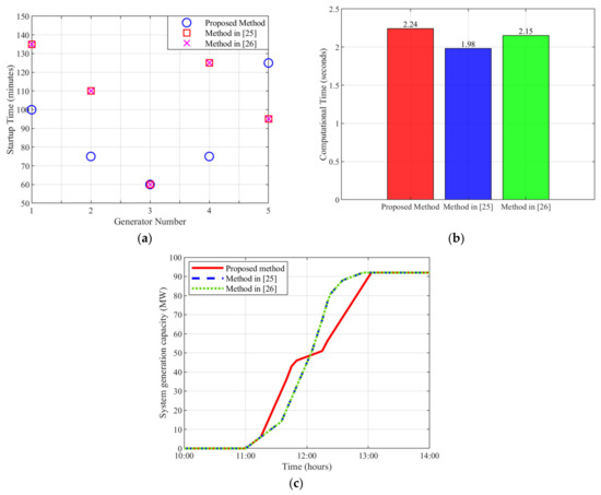
Figure 10.
Comparative analysis of TL-EMS methods on IEEE 39 buses for black start: (a) generator startup times using the two methods against the proposed method; (b) computational time required by the three methods for optimising the black start on IEEE 39 buses; (c) system generation capacity during the black start process. The methods compared include the Proposed method, the method by El-Zonkoly 2015 [25], and the method by Su et al. 2022 [26].
Secondly, a comparative analysis is conducted for the DL-EMS. The proposed unique DL-EMS is evaluated against a similar distribution-level energy management system method described in [27]. Overall, the proposed method demonstrates superiority due to its inclusion of five operational scenarios, including black start and emergency scenarios utilising recent hydrogen fuel cell technology, and its capability to support and connect to the grid. In contrast, the alternative method operates in a standalone manner, includes only three operational scenarios, and lacks both the advanced emergency technology and black start capabilities. Additionally, it fails to optimise the use of solar cells as it neither connects to the grid nor supports supplying excess power to the grid.
Figure 11 illustrates the results of the comparative analysis at the distribution level. Figure 11a presents the outcomes of the method in [27], while Figure 11b shows the results of the proposed method. As depicted in Figure 11a, the battery supports the three loads from 12 AM to 3:30 AM when no sunlight is available. However, the battery reaches 0% SoC, leading to the disconnection of the loads, including the most critical load, due to the absence of an emergency scenario. In contrast, the proposed method includes an emergency scenario and supplies the most critical load during the same period, as shown in Figure 11b. Moreover, as the sun rises and solar power increases, the battery starts recharging and is fully charged by around 12 PM. After this time, the system in [27] must switch the solar power to voltage control mode instead of maximum power point tracking to stabilise the system, resulting in suboptimal use of the excess power. However, the proposed method, being grid-connected, allows the excess power to be delivered to the grid, thereby maximising the utilisation of solar power. Finally, around 9 PM during the night period, the battery discharges again. Without hydrogen fuel cell emergency support, the most critical load will be disconnected, as shown in Figure 11a,b after 9 PM.
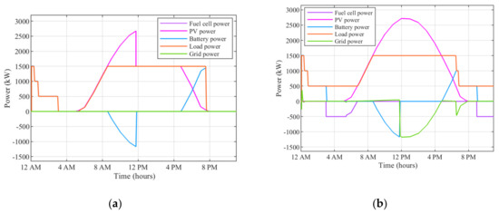
Figure 11.
Comparative analysis of DL−EMS methods: (a) results of methods in [27]; (b) results of the proposed method.
Moreover, a comparison in Table 5 summarises the key aspects of the proposed method and the methods in [25,26,27]. Overall, the results demonstrate the superiority of the proposed method over existing methods in the literature at both the distribution and transmission levels.
Table 5.
Comparison of energy management system methods at distribution and transmission levels.
5. Conclusions
This paper has developed a novel hierarchical energy management system that enhances black start capabilities and normal operations across distribution and transmission networks. The key outcomes and results demonstrate the superior performance of the proposed system in optimising load shedding, system inertia, and renewable energy utilisation during black start events. This was validated using the IEEE 39-Bus test network. The hierarchical control structure, with coordination between distribution and transmission controllers, effectively manages the complex interactions between black start-capable and non-black start-capable areas. It restores essential loads in capable areas first before extending aid to neighbouring areas. The detailed analysis of the multi-area power network architectures provided valuable insights for enhancing power restoration processes, while the innovative objective function, which prioritised renewable energy sources such as solar power, enabled greater integration of sustainable generation into the restored network. This comprehensive framework represents a significant advancement in energy management systems. It addresses key challenges of maintaining grid reliability and resilience. It also enables large-scale integration of renewable generation to drive the transition to a more sustainable energy future.
Author Contributions
Conceptualization, A.C., M.A. and K.A.; methodology, A.C. and M.A.; software, A.C. and M.A.; validation, A.C. and M.A.; formal analysis, A.C. and K.A.; investigation, A.C.; resources, A.C. and K.A.; data curation, A.C.; writing—original draft preparation, A.C. and M.A.; writing—review and editing, A.C. and K.A.; visualization, A.C.; supervision, K.A.; project administration, K.A.; funding acquisition, K.A. All authors have read and agreed to the published version of the manuscript.
Funding
This research received no external funding.
Data Availability Statement
No new data were created or analysed in this study. Data sharing is not applicable to this article.
Conflicts of Interest
The authors declare no conflict of interest.
References
- Sundarajoo, S.; Soomro, D.M. Under voltage load shedding and penetration of renewable energy sources in distribution systems: A review. Int. J. Model. Simul. 2023, 43, 1002–1020. [Google Scholar] [CrossRef]
- Khalid, M. Smart grids and renewable energy systems: Perspectives and grid integration challenges. Energy Strategy Rev. 2024, 51, 101299. [Google Scholar] [CrossRef]
- Alhasnawi, B.N.; Jasim, B.H. A Novel Hierarchical Energy Management System Based on Optimization for Multi-Microgrid. Int. J. Electr. Eng. Inform. 2020, 12. [Google Scholar] [CrossRef]
- Umetani, S.; Fukushima, Y.; Morita, H. A linear programming based heuristic algorithm for charge and discharge scheduling of electric vehicles in a building energy management system. Omega 2017, 67, 115–122. [Google Scholar] [CrossRef]
- Tomin, N.; Shakirov, V.; Kozlov, A.; Sidorov, D.; Kurbatsky, V.; Rehtanz, C.; Lora, E.E. Design and optimal energy management of community microgrids with flexible renewable energy sources. Renew. Energy 2022, 183, 903–921. [Google Scholar] [CrossRef]
- Lissa, P.; Deane, C.; Schukat, M.; Seri, F.; Keane, M.; Barrett, E. Deep reinforcement learning for home energy management system control. Energy AI 2021, 3, 100043. [Google Scholar] [CrossRef]
- Musbah, H.; Ali, G.; Aly, H.H.; Little, T.A. Energy management using multi-criteria decision making and machine learning classification algorithms for intelligent system. Electr. Power Syst. Res. 2022, 203, 107645. [Google Scholar] [CrossRef]
- Musbah, H.; Aly, H.H.; Little, T.A. Energy management of hybrid energy system sources based on machine learning classification algorithms. Electr. Power Syst. Res. 2021, 199, 107436. [Google Scholar] [CrossRef]
- Mosa, M.A.; Ali, A. Energy management system of low voltage dc microgrid using mixed-integer nonlinear programing and a global optimization technique. Electr. Power Syst. Res. 2021, 192, 106971. [Google Scholar] [CrossRef]
- Fu, Z.; Li, Z.; Si, P.; Tao, F. A hierarchical energy management strategy for fuel cell/battery/supercapacitor hybrid electric vehicles. Int. J. Hydrogen Energy 2019, 44, 22146–22159. [Google Scholar] [CrossRef]
- Hu, W.; Wang, P.; Gooi, H.B. Toward optimal energy management of microgrids via robust two-stage optimization. IEEE Trans. Smart Grid 2016, 9, 1161–1174. [Google Scholar] [CrossRef]
- Cagnano, A.; Bugliari, A.C.; De Tuglie, E. A cooperative control for the reserve management of isolated microgrids. Appl. Energy 2018, 218, 256–265. [Google Scholar] [CrossRef]
- Mohiti, M.; Monsef, H.; Anvari-Moghaddam, A.; Lesani, H. Two-stage robust optimization for resilient operation of microgrids considering hierarchical frequency control structure. IEEE Trans. Ind. Electron. 2019, 67, 9439–9449. [Google Scholar] [CrossRef]
- Di Piazza, M.; La Tona, G.; Luna, M.; Di Piazza, A. A two-stage Energy Management System for smart buildings reducing the impact of demand uncertainty. Energy Build. 2017, 139, 1–9. [Google Scholar] [CrossRef]
- Li, J.; You, H.; Qi, J.; Kong, M.; Zhang, S.; Zhang, H. Stratified optimization strategy used for restoration with photovoltaic-battery energy storage systems as black-start resources. IEEE Access 2019, 7, 127339–127352. [Google Scholar] [CrossRef]
- Xu, Z.; Yang, P.; Zeng, Z.; Peng, J.; Zhao, Z. Black start strategy for PV-ESS multi-microgrids with three-phase/single-phase architecture. Energies 2016, 9, 372. [Google Scholar] [CrossRef]
- Fu, Q.; Nasiri, A.; Bhavaraju, V.; Solanki, A.; Abdallah, T.; David, C.Y. Transition management of microgrids with high penetration of renewable energy. IEEE Trans. Smart Grid 2013, 5, 539–549. [Google Scholar] [CrossRef]
- Bazmohammadi, N.; Tahsiri, A.; Anvari-Moghaddam, A.; Guerrero, J.M. Stochastic predictive control of multi-microgrid systems. IEEE Trans. Ind. Appl. 2019, 55, 5311–5319. [Google Scholar] [CrossRef]
- Dao, V.; Ishii, H.; Takenobu, Y.; Yoshizawa, S.; Hayashi, Y. Intensive quadratic programming approach for home energy management systems with power utility requirements. Int. J. Electr. Power Energy Syst. 2020, 115, 105473. [Google Scholar] [CrossRef]
- Bazmohammadi, N.; Tahsiri, A.; Anvari-Moghaddam, A.; Guerrero, J.M. A hierarchical energy management strategy for interconnected microgrids considering uncertainty. Int. J. Electr. Power Energy Syst. 2019, 109, 597–608. [Google Scholar] [CrossRef]
- Tabar, V.S.; Jirdehi, M.A.; Hemmati, R. Energy management in microgrid based on the multi objective stochastic programming incorporating portable renewable energy resource as demand response option. Energy 2017, 118, 827–839. [Google Scholar] [CrossRef]
- Varasteh, F.; Nazar, M.S.; Heidari, A.; Shafie-khah, M.; Catalão, J.P. Distributed energy resource and network expansion planning of a CCHP based active microgrid considering demand response programs. Energy 2019, 172, 79–105. [Google Scholar] [CrossRef]
- Movahednia, M.; Karimi, H.; Jadid, S. Optimal hierarchical energy management scheme for networked microgrids considering uncertainties, demand response, and adjustable power. IET Gener. Transm. Distrib. 2020, 14, 4352–4362. [Google Scholar] [CrossRef]
- Sun, W.; Liu, C.-C.; Zhang, L. Optimal generator start-up strategy for bulk power system restoration. IEEE Trans. Power Syst. 2010, 26, 1357–1366. [Google Scholar] [CrossRef]
- El-Zonkoly, A.M. Renewable energy sources for complete optimal power system black-start restoration. IET Gener. Transm. Distrib. 2015, 9, 531–539. [Google Scholar] [CrossRef]
- Su, J.; Chen, C.; Bie, Z. Optimal Generator Start-Up Sequence Strategy Considering Renewable Energy Participation. In Annual Conference of China Electrotechnical Society; Springer: Berlin/Heidelberg, Germany, 2022; pp. 934–945. [Google Scholar]
- Alassi, A.; Ellabban, O. Design of an intelligent energy management system for standalone PV/battery DC microgrids. In Proceedings of the 2019 2nd International Conference on Smart Grid and Renewable Energy (SGRE), Doha, Qatar, 19–21 November 2019. [Google Scholar]


Disclaimer/Publisher’s Note: The statements, opinions and data contained in all publications are solely those of the individual author(s) and contributor(s) and not of MDPI and/or the editor(s). MDPI and/or the editor(s) disclaim responsibility for any injury to people or property resulting from any ideas, methods, instructions or products referred to in the content. |
© 2024 by the authors. Licensee MDPI, Basel, Switzerland. This article is an open access article distributed under the terms and conditions of the Creative Commons Attribution (CC BY) license (https://creativecommons.org/licenses/by/4.0/).