Abstract
A predictive model for the spatiotemporal distribution of electric vehicle (EV) charging load is proposed in this paper, considering multimodal travel behavior and microscopic traffic simulation. Firstly, the characteristic variables of travel time are fitted using advanced techniques such as Gaussian mixture distribution. Simultaneously, the user’s multimodal travel behavior is delineated by introducing travel purpose transfer probabilities, thus establishing a comprehensive travel spatiotemporal model. Secondly, the improved Floyd algorithm is employed to select the optimal path, taking into account various factors including signal light status, vehicle speed, and the position of starting and ending sections. Moreover, the approach of multi-lane lane change following and the utilization of cellular automata theory are introduced. To establish a microscopic traffic simulation model, a real-time energy consumption model is integrated with the aforementioned techniques. Thirdly, the minimum regret value is leveraged in conjunction with various other factors, including driving purpose, charging station electricity price, parking cost, and more, to simulate the decision-making process of users regarding charging stations. Subsequently, an EV charging load predictive framework is proposed based on the approach driven by electricity prices and real-time interaction of coupled network information. Finally, this paper conducts large-scale simulations to analyze the spatiotemporal distribution characteristics of EV charging load using a regional transportation network in East China and a typical power distribution network as case studies, thereby validating the feasibility of the proposed method.
1. Introduction
The transportation sector is currently undergoing a transition towards low-carbon and intelligent modalities [1]. Electric vehicles (EVs), renowned for their diminished greenhouse gas emissions compared to conventional fuel-powered vehicles, are attracting significant global attention [2]. Projections indicate that EVs will account for approximately two-thirds of the worldwide sales of light-duty vehicles by 2035 [3]. Nevertheless, the escalating ownership of EVs has led to a concomitant rise in energy supply demands, posing significant challenges to the stability of power grid operations. The proliferation of EV charging loads has led to issues such as heightened peak load demand, regional charging bottlenecks, and potential grid overload [4]. The establishment of more precise spatiotemporal distribution models for EV charging loads can facilitate research into the optimization of the deployment and management of EV charging stations [5,6], the operation and control of power distribution networks [7], the utilization and regulation of EV transportation distribution coupled networks [8], and the optimized scheduling of charging and discharging processes [9,10,11], thereby promoting the sustainability of energy resources.
Prior research favored data-driven methods in predicting the spatiotemporal distribution of EV charging loads, which were delineated into two main categories: result data-driven and process data-driven [12]. The former employs intelligent algorithms to predict EV charging loads using extensive temporal series data [13,14,15]. Some studies integrated multidimensional actual influencing factors and proposed collaborative prediction models, further improving the accuracy of short-term load forecasting by considering the correlation between historical data such as transportation, weather, charging stations, trips, and charging behavior [16,17,18]. Challenges persist due to limitations in data reliability stemming from equipment availability, stability of measurements, and privacy concerns. Moreover, many intelligent algorithms utilized in the resulting data-driven method produce prediction models akin to black boxes, complicating quantitative analysis of influencing factors as they store numerous imperceptible data features and lack complete mathematical formulations.
Conversely, the process data-driven method relies on established mature travel statistics to extract potential spatiotemporal travel patterns, ensuring prediction accuracy through effective modeling techniques [12]. In the initial stages of research, scholars primarily focused on analyzing the temporal distribution of EV charging load [19,20]. However, in recent years, there has been an emerging trend among scholars to incorporate travel chain theory to comprehensively consider the spatial distribution of EV charging load. Based on the travel chain theory, References [21,22,23] elucidated the EV travel time, starting and ending locations, number of trips, and trip sequences. However, a common limitation of these studies is that they predefine the structure of travel chains, thereby neglecting the heterogeneity of certain users within the travel chains. Reference [24] treated the travel transfer process of EV users as a Markovian process without memory. Drawing upon Markov theory, these studies proposed spatial transfer probabilities to capture the diversity of travel chains. Additionally, it is worth noting that the spatiotemporal distribution of EV charging load is closely linked to the topological structure of the transportation network. Reference [25] employed a graph-theoretic approach to effectively integrate the power and transportation systems. Supported by travel chains and Markov theory, they proposed a probability model. This model estimates charging demand at network nodes, considering the dynamic spatiotemporal distribution of EVs. References [26,27] enhanced the reliability of the spatiotemporal migration model of EV charging load. They did this by integrating influences from weather conditions and traffic congestion and introducing an energy consumption model. In Reference [28], additional factors such as road grade, saturation level, traffic conditions, classification of streets, and delay at signalized intersections were taken into account. Moreover, a novel algorithm for time-optimal path decision was proposed to optimize the selection of routes. The transportation network information in aforementioned references is predetermined static data, disregarding the real-time interaction between EV trips and traffic flow. Consequently, there may be a mismatch between EV trip simulations and real-time traffic conditions [12]. Reference [29] used travel time of road segments and marginal prices of charging stations. This reflects real-time traffic conditions and dynamic load levels of the power distribution system. A novel real-time charging navigation method was proposed, aiming to minimize overall costs by efficiently locating charging stations. Additionally, adjusting marginal prices can be utilized as a strategy to shift EV load and alleviate real-time traffic congestion. Reference [30] presented an EV spatiotemporal transition model that simulates in incremental steps, capturing the dynamic changes in traffic volume and density throughout the EV spatiotemporal shift process. Notably, the real-time traffic simulation model accurately reflects the interactivity between vehicles, roads, and networks on a micro level, providing a novel modeling approach for the spatiotemporal distribution of EV charging loads.
Table 1 summarizes the considerations of the literature related to this article on different factors.

Table 1.
Summary of the relevant literature.
The current research on the prediction of spatiotemporal distribution of EV charging loads exhibits certain limitations:
- The NHTS2017 statistical data [31] reveal that vehicle travel chains can extend beyond five, while residents’ primary travel purposes can be categorized into eight categories. However, the existing literature lacks a comprehensive analysis of users’ diverse travel behaviors.
- Few studies have focused on the microscopic modeling of EVs traveling in transportation networks. Graph-theoretic-based traffic simulation methods have limitations in accurately describing the real movement characteristics of vehicles and dynamic changes in traffic conditions. Furthermore, traditional single-lane car-following models struggle to reflect the interactivity of vehicles on the road, neglect to account for the intricacies of lane-changing behavior, possess limited capacity to handle traffic congestion, and deviate from real-world situations.
- The existing literature commonly assumes that vehicles start and end their journeys at network nodes, as well as giving little attention to the average vehicle delay caused by traffic signals. Furthermore, real-time traffic information is often not taken into account when determining optimal routes.
In light of the aforementioned research, the current study introduces a predictive model. This model integrates multimodal travel behaviors with microscopic traffic simulation for the spatiotemporal distribution of EV charging loads. Initially, this paper delves into the diverse travel intentions of users, formulating an intricate spatiotemporal model for EV travel. Subsequently, it leverages STCA-II and cellular automata theories to create an advanced multi-lane microscopic traffic simulation model. This model takes into account the average delay per vehicle at intersections, real-time vehicular speeds, and precise origin–destination positions, thus refining conventional path selection methodologies. In the next phase, the model employs a minimum regret value strategy to replicate users’ decision-making at charging stations. It formulates a predictive framework for charging loads, driven by electricity pricing and coupled with real-time network information exchange. Ultimately, this paper ascertains the spatiotemporal distribution of EV charging loads through extensive vehicle simulation analyses.
2. EV Travel Spatiotemporal Model
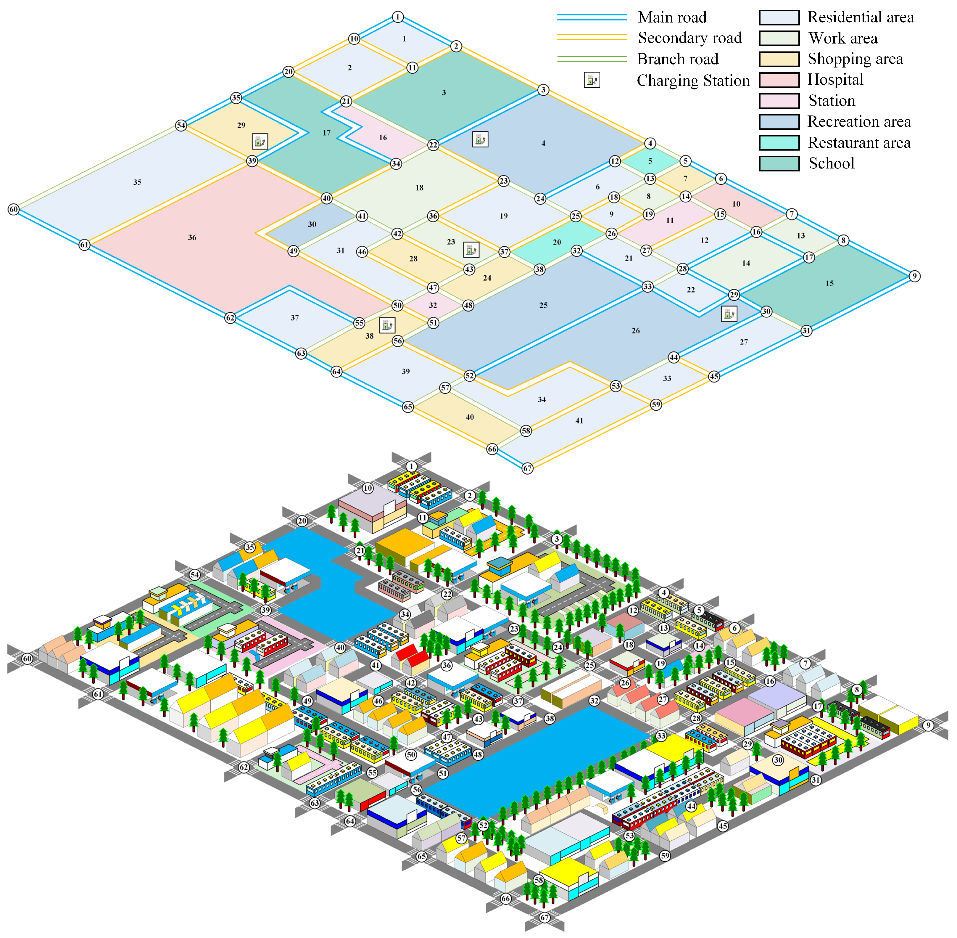
The transportation network of a specific region in East China is depicted in Figure 1. Furthermore, the length data pertaining to the transportation network can be found in Table A1, Appendix A.

Figure 1.
Schematic diagram of regional transportation network.
The spatiotemporal characteristics of EVs can be effectively analyzed by leveraging traditional household travel survey data [32]. Additionally, it has been observed that users exhibit a higher frequency of travel activities on weekdays compared to holidays [33]. Simultaneously, private cars and taxis play pivotal roles in urban transportation. Therefore, this study focuses on electric private cars and electric taxis during weekdays as the primary research subjects, based on the NHTS 2017 statistical data. Furthermore, an EV travel spatiotemporal model is developed.
2.1. Distribution of Initial Travel Time and Location
To enhance the precision of the model, a Gaussian mixture distribution is employed instead of the conventional normal distribution to fit the initial travel time of EVs. The fitting results are illustrated in Figure 2.
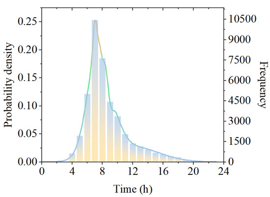
Figure 2.
Probability distribution of initial travel time.
The distribution probability of the initial travel location pertains to the probability distribution of users in various functional areas during their initial travels, as depicted in Table 2.
Table 2.
Probability distribution of initial travel time.
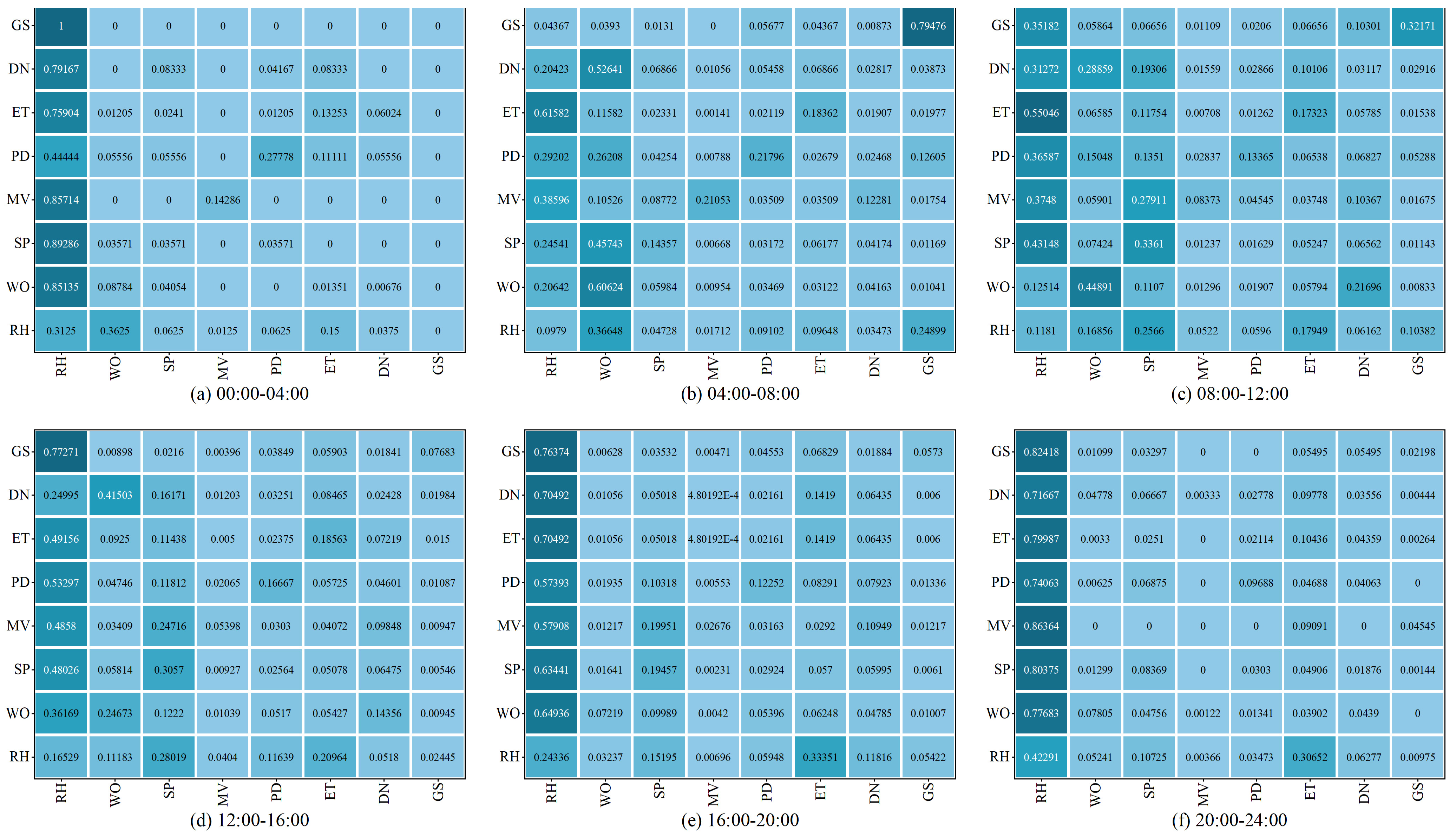
2.2. Travel Purpose Transfer Probability
The purposes of user travel can be categorized into eight categories, namely: return home (RH), work (WO), shopping (SP), medical visits (MV), pick-up/drop-off (PD), entertainment (ET), dining (DN), and going to school (GS), corresponding to eight functional areas.
By applying the principles of Markov theory, travel purposes are treated as distinct states, where the subsequent state is solely determined by the current state [23]. The travel purpose transfer probability matrix of EVs at period t is presented in (1) and (2).
where represents the single-step transfer probability from travel destination X to travel destination Y at period t.
The travel purpose transfer probability matrix during different periods is shown in Figure 3.

Figure 3.
Travel purpose transfer probability matrix during different periods.
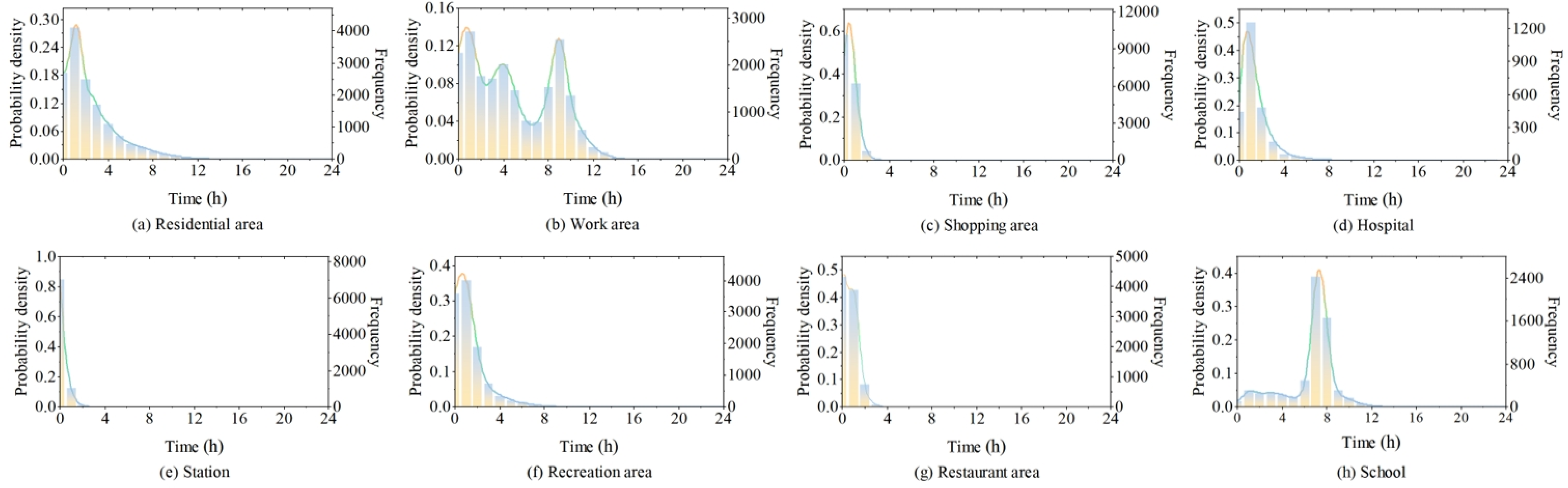
2.3. Duration of Parking in Different Functional Areas
The fitting results of the duration of parking in different functional areas are illustrated in Figure 4. Gaussian mixture distribution is employed to fit the duration of parking in residential areas, work areas, stations, recreation areas, restaurant areas, and schools. Logistic distribution is utilized to fit the duration of parking in shopping areas. Generalized extreme value distribution is applied to fit the duration of parking in hospitals. Compared to the traditional methods commonly employed in the prior literature, such as fitting with normal or exponential distributions, the approach utilized in this study exhibits superior goodness of fit and enables a more precise depiction of the distribution of time variables. It is worth mentioning that the duration of parking in residential areas here pertains to the duration of brief stays at home before resuming daily travel, without factoring in the initial point of travel chains.
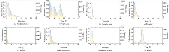
Figure 4.
Probability distribution of duration of parking in different functional areas.
3. Microscopic Traffic Simulation Model
To improve the accuracy of vehicular traffic simulations on bidirectional multi-lane roadways, the present research integrates the STCA-II model [34]. This advanced model abstracts the transportation network into a grid of discretely arranged cells, thereby facilitating the execution of dynamic traffic flow simulations via a sophisticated traffic flow cellular automaton framework.
3.1. Vehicle Evolution Update Rules Based on the STCA-II Model
The procedures for the evolution and update of vehicles en route to their destination are as follows:
- Lane-changing Behavior Update
When a vehicle is unable to reach its target speed within the confines of the current lane, yet the conditions of the adjacent lane are conducive to meeting its acceleration needs, a probabilistic lane change is executed. The motivation for lane changing and the safety conditions are, respectively, presented in (3) to (4) and (5).
where represents the distance between vehicle i and the preceding vehicle in lane s at time t; Δt is the time step interval, set to 1 s; denotes the traveling speed of vehicle i in lane s at time t; A denotes the acceleration of the vehicle per second, which can be approximated as 1 [34]; is the maximum speed limit of the road r where the vehicle is located; Equation (3) indicates a conflict between the distance of vehicle i to the preceding vehicle and its acceleration expectation; represents the distance between vehicle i and the preceding vehicle in the adjacent lane s at time t; Equation (4) implies that the distance between vehicle i and the preceding vehicle in the adjacent lane is greater than the distance to the preceding vehicle in the current lane. This suggests that a lane change would satisfy the acceleration expectation of vehicle i; represents the distance between vehicle i in lane s and the trailing vehicle in the adjacent lane at time t; Equation (5) assumes that the trailing vehicle in the adjacent lane to vehicle i is moving forward at velocity , thereby ensuring the safety of vehicle i during the lane-changing process.
The absence of vehicles driving in parallel lanes is also a prerequisite for lane changing. The transportation network analyzed within this investigation is composed predominantly of two-lane and three-lane thoroughfares. The leftmost lane is designated for left turns and straight movements, the rightmost lane for right turns and straight movements, while the middle lane is intended for through traffic. Vehicles enter and exit the network via the rightmost lane. As drivers approach a signalized intersection, they will determine their turning maneuvers based on their intended route, merging into the appropriate lane well in advance. It is also observed that lane-changing activity is suspended prior to the driver’s departure from the intersection.
- 2.
- Acceleration Behavior Update
The acceleration rule characterizes the psychological activity of users who expect to travel on road r at the maximum possible speed, , as depicted in (6).
- 3.
- Deceleration Behavior Update
The deceleration rule represents the psychological activity of users avoiding risk, as delineated in (7).
- 4.
- Stochastic Deceleration Behavior Update
The stochastic deceleration rule characterizes the behavior of users randomly slowing down due to uncertain factors, as demonstrated in (8).
where pMod represents the probability of stochastic deceleration, set to 0.1.
- 5.
- Location Update
The position update rule characterizes the iterative movement characteristics of the user’s location with respect to time steps, as indicated in (9).
where denotes the position of the i-th vehicle on road r at time t. When it exceeds the length of road r and the corresponding phase at the signalized intersection is green, transit time within the intersection is disregarded, allowing for the vehicle to proceed to any lane within the next group of lanes. Conversely, if the signal is not green, the vehicle will come to a halt before reaching the intersection and set = 0.
3.2. Optimal Path Decision-Making Considering Signal Intersection Delays, Real-Time Vehicle Speeds, and Start–Stop Positions
The start–stop positions of a vehicle frequently do not coincide with network nodes but are situated along intermediary segments of the roadway. Due to differences in real-time traffic flow and road capacity, signal intersection delays vary depending on the chosen driving routes. Assuming U-turns are allowed on any road, let q represent the number of network nodes, ϒ denote the road weight matrix, and Λ demonstrate the average speed matrix of lane groups over the nearest 15 min interval at time t. If node a and node b are not adjacent, then Λ(a,b) = 0 and ϒ(a,b) = 0. The steps for optimal path decision-making are as follows:
- Step1
Treat the origin and destination points as new network nodes, denoted as q + 1 and q + 2, respectively, then insert them into their respective origin and destination roads. Each of these roads is divided into two new segments, with each segment inheriting the average speed of the lane group from the previous 15 min on the original road, along with phase information regarding interactions with adjacent roads at both ends of the original road. Notably, there is no signal intersection delay between newly created segments resulting from the same division.
- 2.
- Step2
Initialize the routing matrix Z; initialize the optimal time matrix T, as presented in (10).
- 3.
- Step3
Based on the Floyd algorithm, the iterative updating of matrices T and Z is accomplished, with the pseudocode delineated in Algorithm 1. Herein, the average delay at signalized intersections is computed utilizing the HCM1985 delay model [35], as illustrated in (11).
where εh represents the average delay at signalized intersections for lane group h (s); HT denotes the signal cycle duration (s); Fh refers to the green ratio for lane group h; σh signifies the saturation level for lane group h; φh is the capacity of lane group h (pcu/h).
| Algorithm 1: Pseudocode of improved Floyd algorithm (Procedure) |
| for k = 1 : q + 2 for a = 1 : q + 2 for b = 1 : q + 2 if T(a,k) ≠ inf & T(k,b) ≠ inf & a ≠ k & k ≠ b & k ≠ q + 1 & k ≠ q + 2 then By utilizing Z, the current optimal path from node a to node k can be computed and the preceding node k’ of node k can be retrieved The vehicle’s location in terms of road and lane group is determined based on nodes k and k’, facilitating the extraction of corresponding HT, Fh, σh, and φh Calculate εh by (11) else εh = 0 end if if T(a,b) > T(a,k) + T(k,b) +εh then T(a,b) = T(a,k) + T(k,b) +εh Z(a,b) = k end if end for end for end for |
3.3. Unit Distance Energy Consumption Model
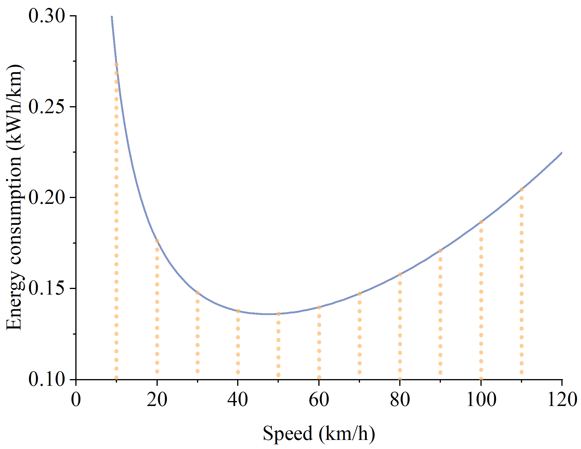
The unit distance energy consumption is closely related to the distance and speed at which EVs travel on various roads. Many studies often treat it as a constant value, which may introduce a certain degree of error in prediction outcomes. Therefore, this study incorporates the unit distance energy consumption model from References [36,37] into the traffic flow cellular automaton model to accurately calculate the real-time energy consumption of EVs during their operation, as depicted in (12).
where er represents the energy consumption per unit distance of an EV traveling on road r (kWh); is the average speed of the EV on road r (m/s); ρ denotes the air density, assumed to be 1.2 kg/m3; is the drag coefficient, with a value of 0.29; ϖ is the frontal area of the vehicle facing the wind, taken to be 2.27 m2; μ is the friction coefficient, with a value of 0.012; Mev is the weight of the EV, assumed to be 2000 kg; g is gravitational acceleration, taken as 9.81 m/s2; θ is the road grade, assumed to be 0°; ϛ is the efficiency parameter, with a value of 0.9; Pacc is the energy consumption of auxiliary systems, assumed to be 2 kW.
The relationship between energy consumption per unit distance and speed is illustrated in Figure 5.
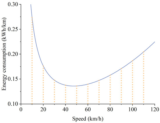
Figure 5.
The relationship between energy consumption per unit distance and speed.
4. Predictive Framework for Spatiotemporal Distribution of EV Charging Load with Real-Time Information in Traffic-Power Coupled Network
The integration of advanced technologies, including big data, 5G communication, cloud computing and vehicular internet, has facilitated instantaneous information exchange between users and interconnected networks [38]. On one hand, the real-time operational status of interconnected networks can serve as a fundamental basis for establishing dynamic electricity pricing. On the other hand, leveraging intelligent systems enables users to access real-time information on electricity prices, occupancy rates, and traffic conditions across diverse charging stations, facilitating informed decision-making for optimal station selection.
4.1. Electricity Pricing Model Considering the Secure Operation of Power Distribution Networks
The concentrated charging of EVs during periods of high initial load in the power distribution network can give rise to a phenomenon referred to as peak overlapping. Therefore, setting charging tariffs that change depending on the surplus or shortfall compared to the average load in the power distribution network at different times is a practical solution. Moreover, persisting with elevated charging loads amidst periods of diminished regional nodal voltages has the potential to diminish the power generation system’s supply capacity. Consequently, it is possible to regulate the charging tariffs upwards in areas with lower voltages, thereby effectively directing EVs towards charging in diverse areas and mitigating the deterioration of nodal voltage quality [39]. To mitigate the computational burden, this paper disregards the influence of extraneous variables and employs the depicted strategy for establishing charging prices as subsequently outlined.
where ct represents the real-time charging price at time t; cb denotes the base charging price, set at 1 CNY/kWh; ι refers to the time-varying price adjustment factor, set at 1/3; Pt signifies the original load of the power distribution network at time t; is the average load of the power distribution network; indicates the charging price for region α at time t; is the regional price adjustment factor, set at 5; corresponds to the per unit value of voltage at the power distribution network bus that region α is connected to at time t; Ts is the total number of periods into which the day is divided, set at 96.
4.2. Charging Station Decision Model Based on Regret Theory
Regret theory can effectively capture the psychological traits of decision-makers who strive to minimize regret and maximize benefits, thereby closely aligning with users’ genuine cognitive patterns [40]. When users make decisions regarding charging stations, the total regret value represents the comparison of composite utility at time t when selecting between charging stations m and n, which can be computed using (16) to (21).
where denotes the time utility regret value generated at time t when selecting charging station n in comparison to charging station m; if the vehicle is a private car, and , respectively, represent the expected time for the user to go to charging stations m and n for charging, until reaching the next destination; if the vehicle is a taxi, and , respectively, represent the expected time for the user to go to charging stations m and n for charging, until the end of charging; denotes the economic utility regret value at time t when selecting charging station n in comparison to charging station m; and are the respective economic costs incurred by the user when completing charging at charging stations m and n; represents the user’s value of unit time, with private cars and taxis having respective values of 0.370 CNY/min and 0.321 CNY/min; , and , and represent the driving time to charging station m, the queuing time at charging station m, the charging time, and the driving time from charging station m to the next destination, respectively. It is important to note that, since taxis do not have a predetermined next destination, it is assumed that = 0; denotes the equivalent conversion value between hours and minutes, = 60; Cbat denotes the battery capacity of the EV; Sid represents the user’s ideal state of charge (SOC), which can be approximately set at 0.85 based on user investigation findings; refers to the SOC of the user upon arrival at charging station m, which must be ensured to be greater than 0 for charging station m to be considered as a potential option; η denotes the charging efficiency, set at 0.95; stands for the rated charging power of charging station m; and represent the time when charging starts and finishes, respectively; indicates the electricity price for charging at charging station m at time t; represents the parking fee incurred by the user when charging is completed at charging station m. All aforementioned time parameters are measured in minutes.
The final regret value for a user selecting charging station m is determined as the maximum among the total regret values calculated in comparison with the selection of other alternative charging stations. Moreover, the user should select the final plan based on the minimum regret value Gt, as indicated by (22) and (23).
where ncs represents the identification number of the alternative charging stations; Ncs denotes the total number of charging stations.
4.3. Spatiotemporal Distribution Predictive Framework for EV Charging Load
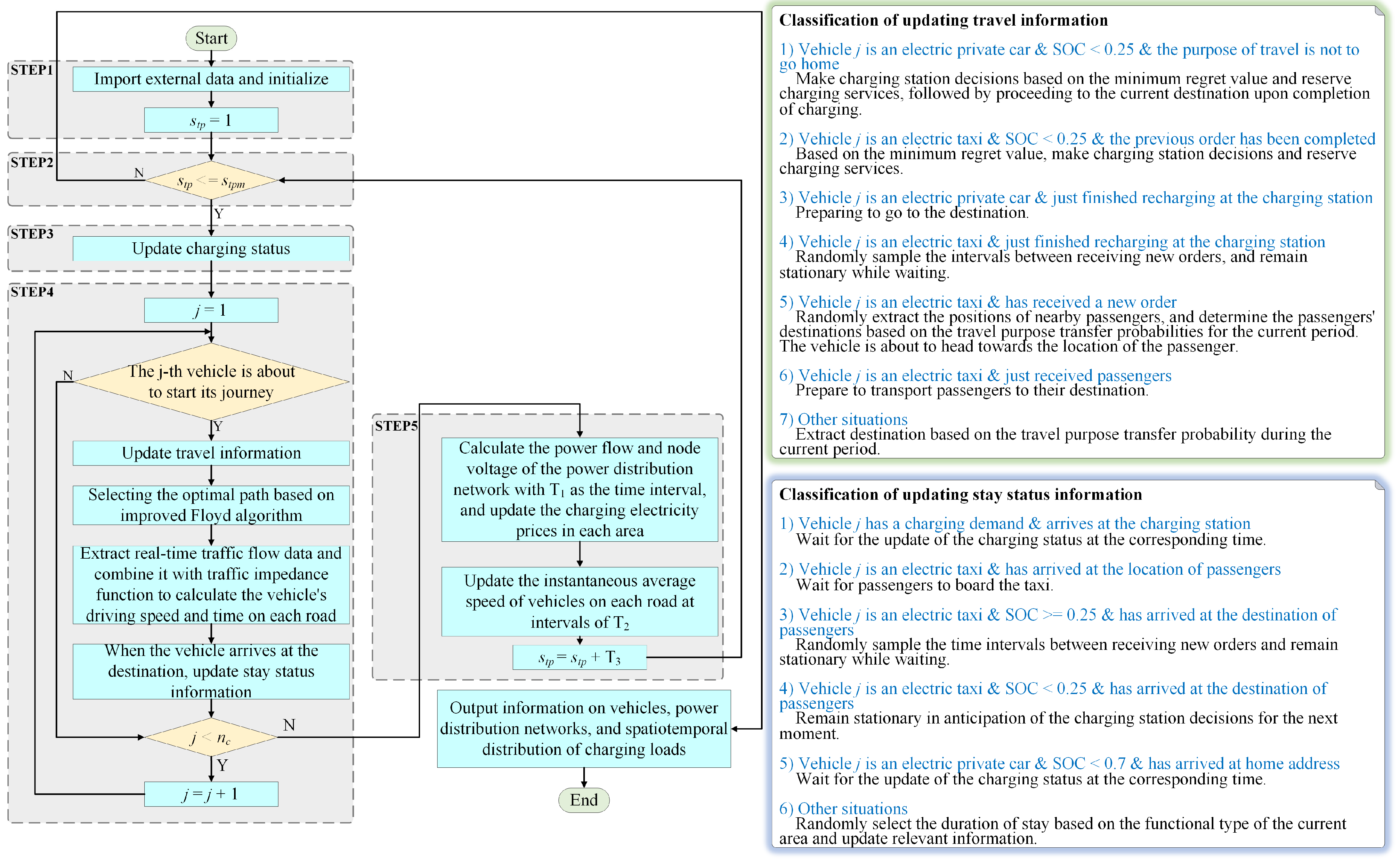
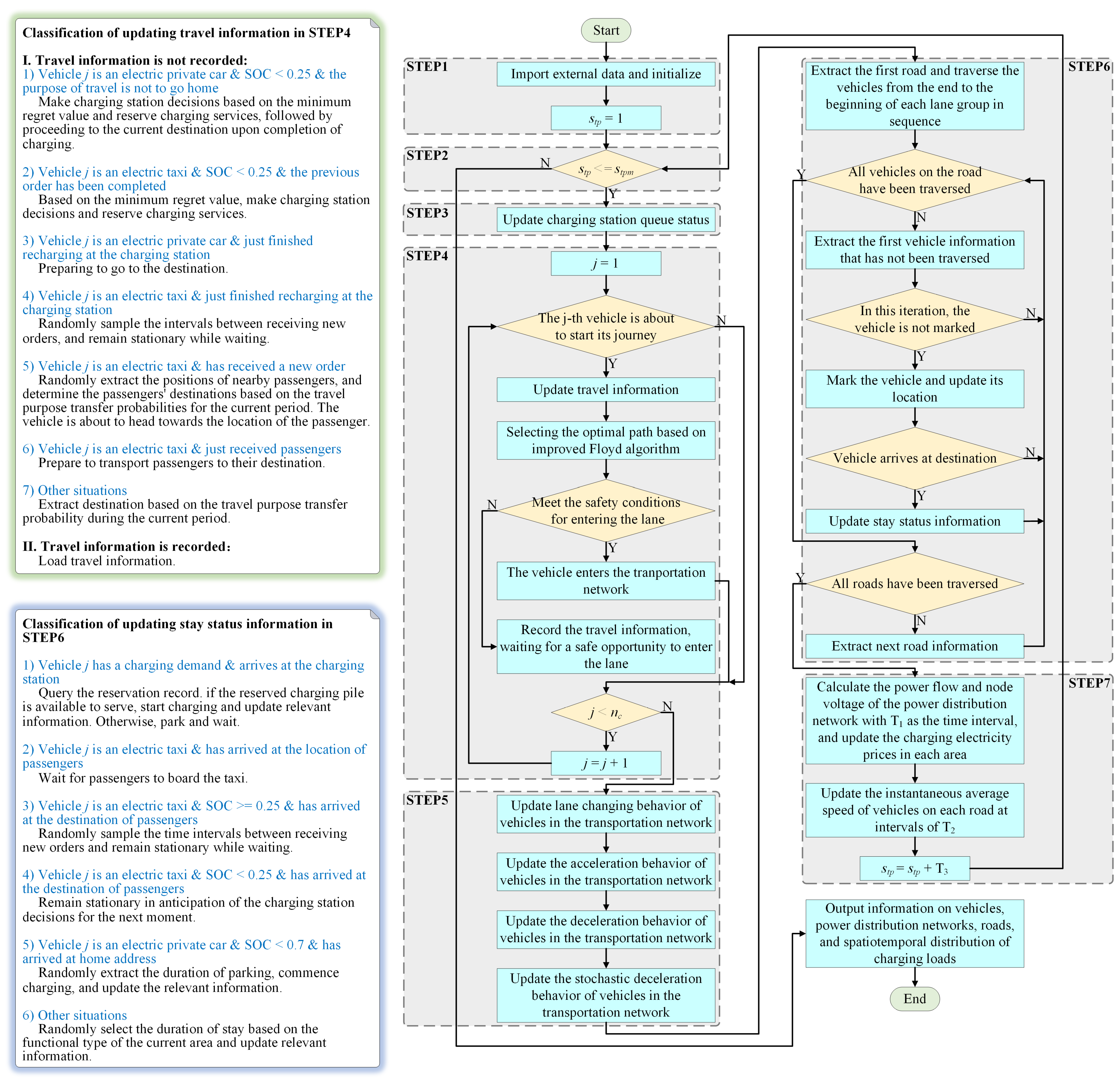
The simulation process for the spatiotemporal distribution of EV charging load is illustrated in Figure 6, with the detailed steps following.
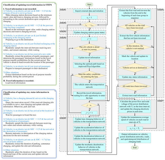
Figure 6.
The simulation process for the spatiotemporal distribution of EV charging load.
- Step1
Import external data, initializing parameters including vehicle status, initial travel time, residential and workplace addresses, electricity tariffs, simulation time (stp), as well as the maximum simulation duration (stpm), among others.
- 2.
- Step2
If stp <= stpm, proceed to Step3. Otherwise, output relevant information and conclude the simulation.
- 3.
- Step3
Update the queuing status of the charging station. If EVs are waiting for charging while their reserved charging piles are available to serve them, update the status of the EVs and the information on the grid side.
- 4.
- Step4
Determine the travel status of vehicle j based on stp, update its travel information, and assess whether it can safely merge into the lane at the current moment until j surpasses the total number of vehicles nc.
- 5.
- Step5
Update the lane-changing behavior, acceleration behavior, deceleration behavior, and stochastic deceleration behavior of vehicles in the transportation network.
- 6.
- Step6
Update the positions of vehicles in the transportation network.
- 7.
- Step7
With T1 as the time interval, conduct power flow and bus voltage calculations for the power distribution network and update the charging electricity prices for each area. With T2 as the time interval, update the instantaneous average speed of vehicles on each road; T3 is the simulation time step; set stp = stp + T3 and return to Step2.
5. Case Analysis
5.1. Parameter Settings
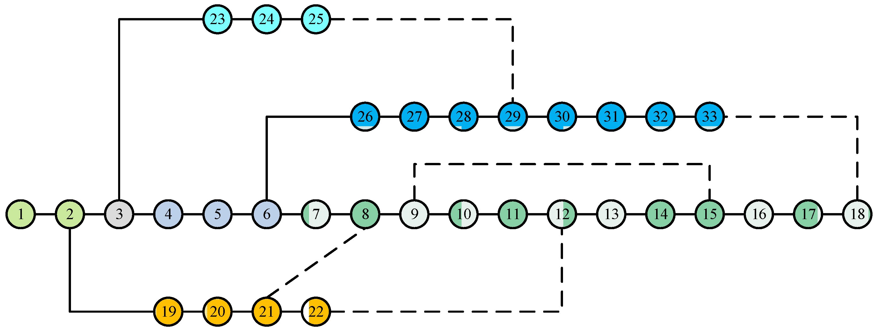
The coupling relationship between power distribution network and areas, as well as the configuration parameters of charging stations, are illustrated in Table 3 and Table 4, respectively. The experimental power distribution network employed in this study is derived from the IEEE 33-bus system, with line parameters judiciously modified to ensure capacity alignment with the regional scope under consideration. Figure 7 depicts the schematic representation of the power distribution network’s configuration.
Table 3.
Coupling relationship between power distribution network and areas.
Table 4.
Configuration parameters of charging stations.
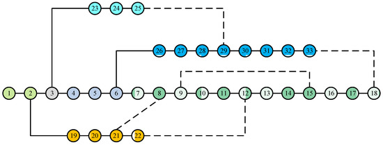
Figure 7.
Schematic representation of the power distribution network’s configuration.
The residential areas are assumed to be equipped with comprehensive charging facilities, with a basic charging power of 7 kW, accommodating a total of 30,000 vehicles. This comprises 23,200 conventional private cars, 6000 electric private cars, and 800 electric taxis. The zero-flow speeds for main roads, secondary roads, and branch roads are set at 60 km/h, 40 km/h, and 30 km/h, respectively. Each road type consists of three lanes for main roads and secondary roads while branch roads have two lanes. The unit cell length is considered as 1 m. The time intervals T1, T2, and T3 are defined as 15 min, 10 s, and 1 s, respectively. Electric private cars initially possess SOC values following a uniform distribution U(0.7,1), whereas electric taxis follow a uniform distribution U(0.2,0.85) for their initial SOC values. The interval between order pickups for electric taxis (in minutes) follows a uniform distribution U(0,10). All EVs have a capacity of 60 kWh.
The Monte Carlo method is utilized to simulate the spatiotemporal distribution of charging load from Monday to Friday. Under consistent simulation parameters, the predictive results are compared with those obtained using a graph-theoretic predictive method. The simulation process and detailed steps of the graph-theoretic predictive method can be found in Appendix B. It should be noted that in replicating the graph-theoretic predictive method, a traffic impedance function [41] is employed to simulate real-time vehicular speeds on the roads. Furthermore, for the initial trip of the subsequent day with a residential area as its destination, the duration of parking is determined based on the initial travel time of that day’s first travel [24].
5.2. Simulation Results Analysis
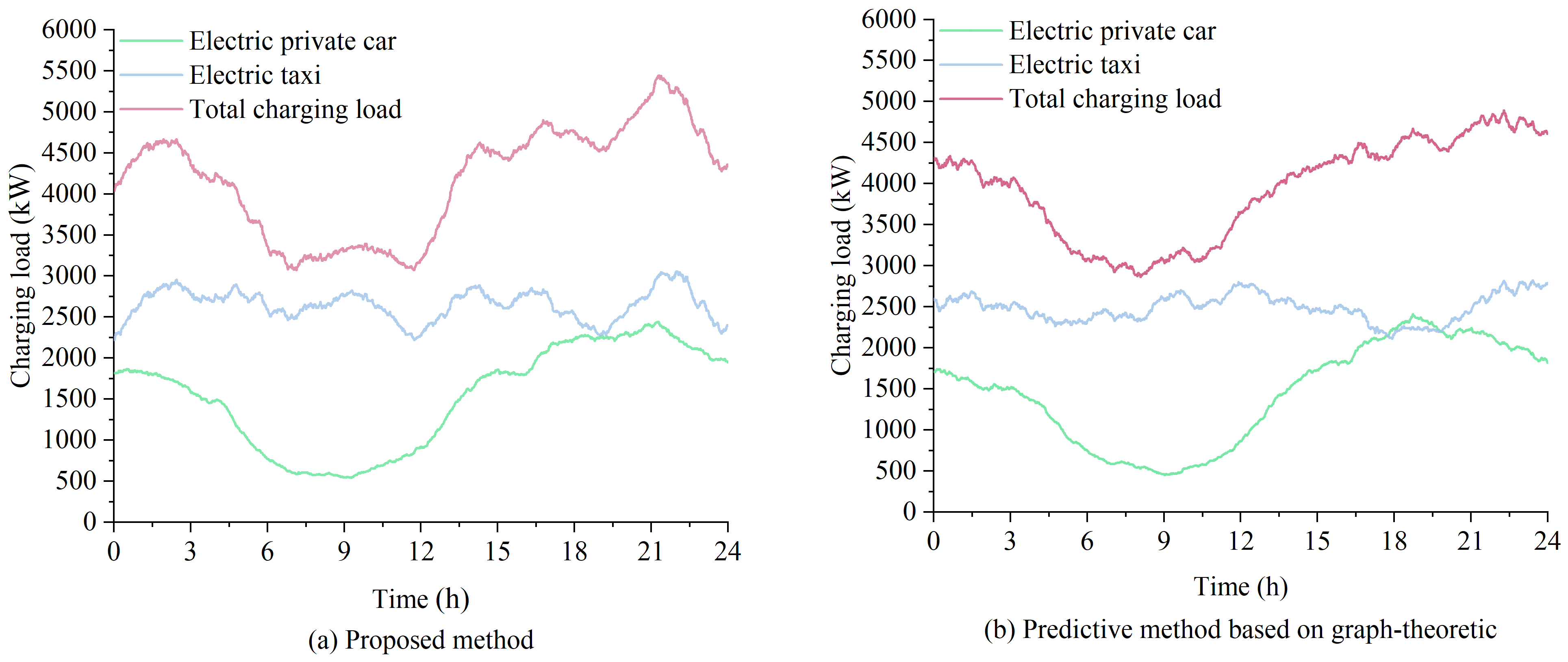
The temporal distribution of the daily average charging load for EVs under the two methods is illustrated in Figure 8. According to the findings derived from the graph-theoretic prediction method, the root mean square error (RMSE) and mean absolute error (MAE) of the proposed method are computed with a time resolution of 1 min, as illustrated in Table 5. The methodologies used to compute RMSE and MAE are detailed in Reference [42] and will not be further expounded upon here. The temporal distribution curve of the charging load, as obtained through our proposed method, exhibits a consistent daily variation trend with that predicted by the graph-theoretic-based method. Notably, the RMSE and MAE associated with our method are relatively low, underscoring its reliability in predicting the temporal distribution of EV charging load. Furthermore, the prediction results of the proposed method exhibit more pronounced fluctuations. In previous studies, the distribution of vehicles arrival times at their destinations are more stable because the simulation of vehicle speed using the velocity flow model in graph theory is considered from a macro perspective. This method is relatively ideal and deviates from the actual situation. However, from the perspective of microscopic traffic simulation, the speed of vehicles on the road changes in real time, affected by a variety of factors, and traffic signals at intersections can also cause some delays in actual travel times. Therefore, the actual traffic situation will have a certain impact on the distribution of EV charging loads.
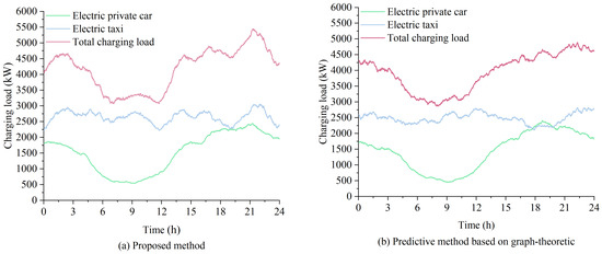
Figure 8.
Temporal distribution of the daily average charging load for EVs: (a) proposed method; (b) predictive method based on graph-theoretic.
Table 5.
RMSE and SAE of the proposed method.
As can be seen from Figure 8a, the charging load of electric private cars exhibits a significant peak-to-valley difference, with the peak period occurring between 18:00 and 22:00. This phenomenon reflects the behavior of electric private car users who tend to charge their vehicles in residential areas after returning from work. Electric taxis, on the other hand, display a relatively small peak-to-valley difference in their charging load. Their charging demand is higher than that of electric private cars and their charging load curve is relatively flat, concentrated between 2 MW and 3 MW. Overall, the charging load of EVs demonstrates high volatility, with a peak-to-valley difference of approximately 2.377 MW. The highest load peak occurs around 21:17 at approximately 5.444 MW, while the lowest load point is observed around 7:08 at approximately 3.067 MW. Notably, additional load peaks emerge around 2:00, 14:00, 17:00, and 21:00. Conversely, the period from 7:00 to 12:00 represents a low-load valley period.
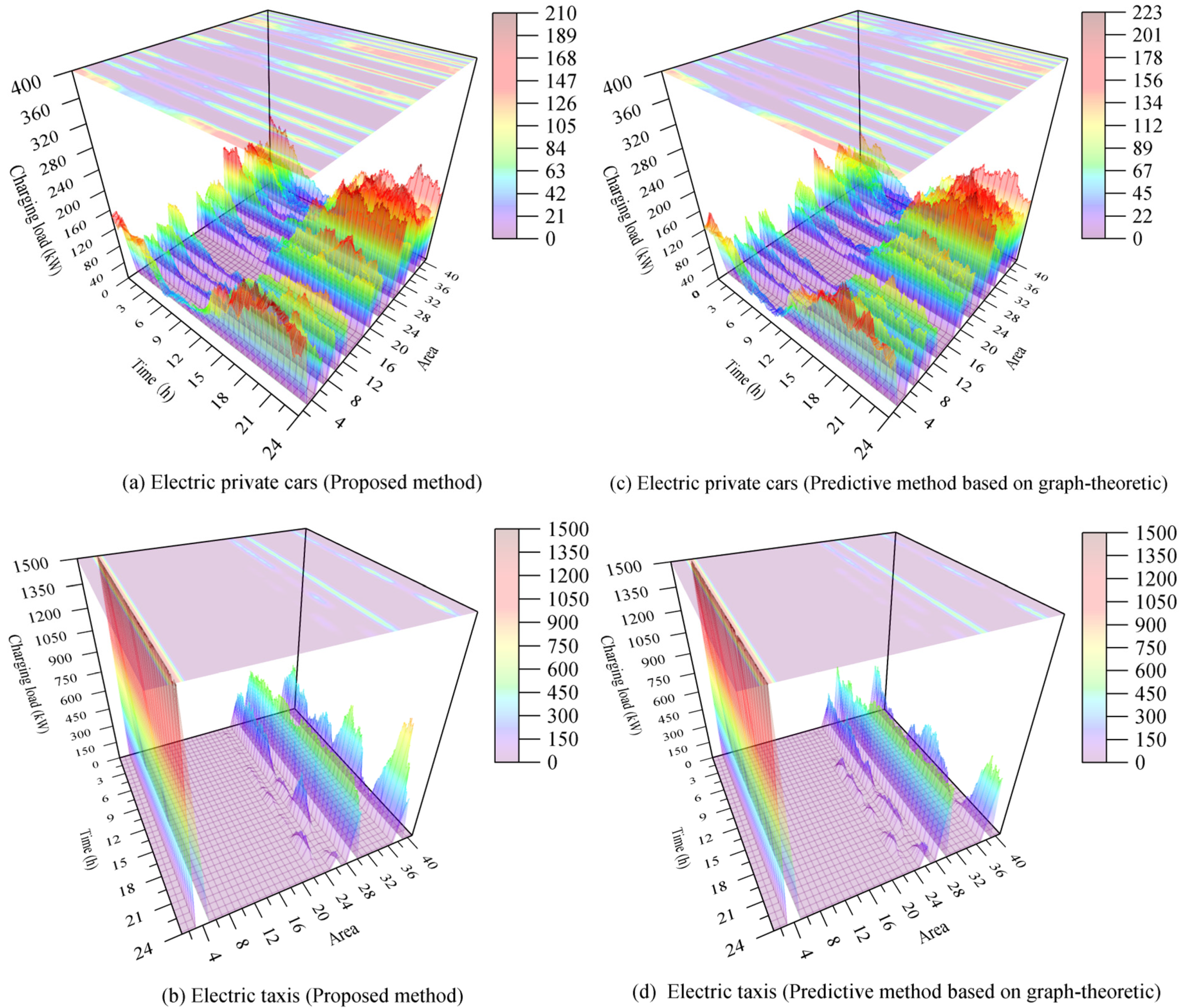
The spatiotemporal distribution of the daily average charging load of EVs for both methods is shown in Figure 9. In both cases, the charging load distribution of private electric cars within each functional area exhibits a similar pattern, primarily concentrated during the afternoon and evening hours. Notably, the charging load distribution of electric taxis at various charging stations is roughly the same, with some minor differences in the load distribution at a few charging stations during certain periods. These discrepancies arise due to limitations inherent in graph-theoretic approaches that do not fully account for microscopic vehicle simulation, resulting in deviations when estimating driving energy consumption and time. Under these circumstances, users’ charging station decisions will also be affected to some extent.

Figure 9.
Spatiotemporal distribution of the daily average charging load of EVs: (a) electric private cars (proposed method); (b) electric taxis (proposed method); (c) electric private cars (predictive method based on graph-theoretic); (d) electric taxis (predictive method based on graph-theoretic).
Figure 9 illustrates that the charging load curves of electric private cars in each residential area exhibit a consistent variation trend with their overall charging load curve. The differences in charging loads among residential areas are primarily influenced by the distribution of electric private cars. The charging load at charging stations mainly comes from electric taxis, and there are also significant differences in the charging load distribution among the charging stations. Charging station 1 experiences high charging loads, with occupancy rates near 100% at all times. This is because charging station 1 is connected to the balanced node of the power distribution network, which has a higher bus voltage. As a result, charging prices are relatively lower, and parking fees are also reduced. Consequently, users opting for charging station 1 typically incur substantial economic savings. Charging station 4 similarly garners user preference due to its consistently competitive charging prices, with its occupancy rates ranking second to charging station 1. Nevertheless, this also leads to a situation where charging stations 1 and 4 often have a large number of EVs queuing up. In comparison, charging stations 3 and 5 exhibit greater volatility in their charging load, characterized by a multi-peak distribution pattern and pronounced variations in occupancy rates across different time intervals. The charging load of charging station 2 is the lowest, primarily due to its comparatively higher charging prices and parking fees. Even when charging stations 1 and 4 experience queues, the combined cost of selecting charging stations 3 and 5 is generally lower than that of opting for charging station 2. In accordance with the charging price framework established in this paper, certain stations may entice an influx of EVs attracted by their lower total costs, thereby precipitating queues for some patrons. However, there might also be charging stations with high total costs experiencing prolonged periods of idle charging piles. Hence, subject to meeting specific conditions, the strategic expansion of select charging stations could be instrumental in curtailing the wait times for users in queues. Furthermore, the introduction of a pricing adjustment factor at some stations, through the reduction of charging costs or parking fees, could lure users to these locations, thus distributing the EV load more reasonably among the stations.
The average daily charging cost, average daily number of charges, average daily charging capacity, and average daily parking cost of each EV obtained by the two methods are presented in Table 6. It can be observed that the various indicators under both methods exhibit similar trends, thereby further validating the reliability of the proposed method in this study. Notably, the indicators derived from our proposed method slightly surpass those obtained using a graph-theoretic approach. This disparity can be attributed to the more precise simulation of EV energy consumption through microscopic traffic simulation, which better accommodates the variability in EV driving behavior on real roads. The data suggest that the daily travel requirements for electric private vehicles are modest, with a significant dispatchable capacity accessible for the majority of time intervals. Conversely, electric taxis exhibit a more substantial demand for charging and constitute a primary contributor to the power grid load. In the interest of augmenting the capability of electric taxis to contribute to public transport services, strategies such as elevating the charging capacity at stations, modulating electricity tariffs to diminish the idleness of charging infrastructure, and broadening the network of charging facilities can be contemplated. These measures aim to decrease the aggregate recharging duration for electric taxis.
Table 6.
Average daily charging cost, average daily number of charges, average daily charging capacity, and average daily parking cost of each EV.
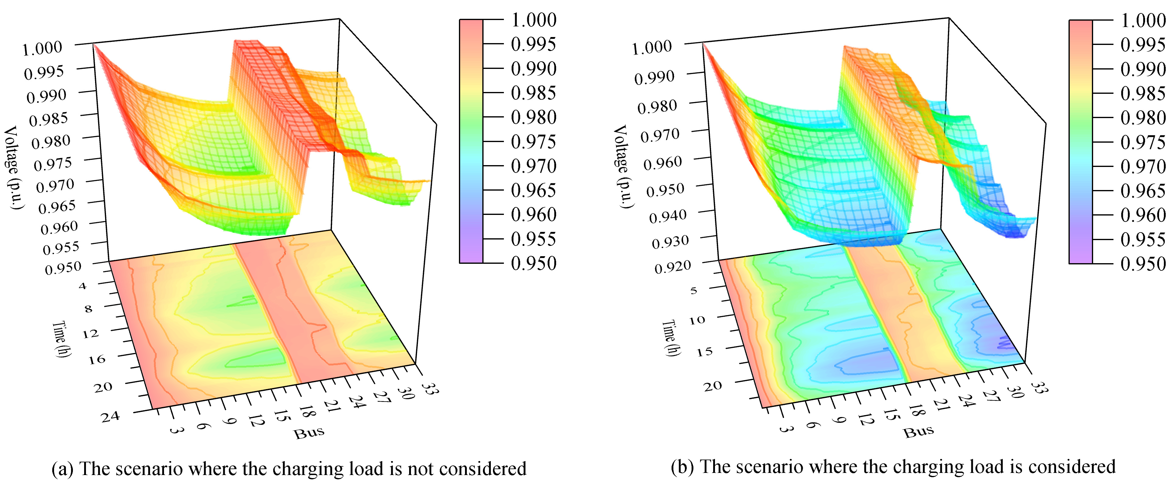
The bus voltage distribution in the power distribution network, both before and after considering the charging load, is illustrated in Figure 10, while specific voltage drop values for selected buses are presented in Table 7. It is evident that the integration of EVs leads to varying degrees of voltage reduction across the distribution network buses, with the minimum nodal voltage decreasing from 0.977 3 p.u. to 0.958 9 p.u. Notably, the bottom projection of buses 6 to 18 and 26 to 33 shifts from a predominance of yellow–green to a predominance of green–blue. During peak load periods, the bottom projection of some buses even exhibits a light purple hue, indicating voltages dropping to approximately around 0.96 p.u. Clearly, it can be concluded that EV charging loads significantly impact the power quality of the power distribution network and should be duly considered when formulating relevant dispatch policies.
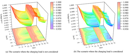
Figure 10.
Bus voltage distribution of the power distribution network: (a) the scenario where the charging load is not considered; (b) the scenario where the charging load is considered.
Table 7.
Voltage drop values for selected buses (p.u.).
In summary, when selecting travel routes, EV users take into account real-time traffic conditions. In situations of urgent charging needs, the recommended route by the optimal charging station decision will affect the traffic conditions over the upcoming period. The utilization of microscopic traffic modeling enhances the interactivity between EVs and the road network, thereby improving the reliability of simulations for actual driving time and energy consumption. The charging load of EVs exhibits significant variability, with lower loads observed during mornings on workdays compared to other periods. Temporal distribution characteristics of charging loads in residential areas are similar and primarily depend on EV ownership within each area. The occupancy rate of charging piles at charging stations is closely linked to electricity prices and parking fees. Developing appropriate electricity pricing policies for different charging stations can mitigate user clustering for charging purposes and enhance urban transportation efficiency. Electric private cars remain idle for most of the day and possess substantial dispatchable capacity, making them a key reserve force capable of participating in orderly charging and discharging activities in the future. The impact of EV charging load on power distribution network safety is significant. Various electrical quantities’ variations should be considered in future research.
6. Conclusions
This paper presents a predictive framework for spatiotemporal distribution of EV charging load that is based on multimodal user travel and microscopic simulation. The framework is characterized by the following features:
- A refined spatiotemporal model for EV travel was established. From a temporal perspective, the distribution of EV travel time variables is described more accurately. From a spatial perspective, the multimodal of user travel and the diversity of functional areas are fully taken into account.
- The construction of a sophisticated microscopic simulation system for transportation networks is based on the multi-lane cellular automaton model. In contrast to conventional approaches that rely on graph-theoretic methods to describe the macroscopic topology of transportation networks, this methodology enables a more realistic representation of intricate vehicle movements within the network.
- Supported by real-time information exchange within the coupled network, the optimal path decision-making process takes into account the scenarios where the EV’s starting and ending positions are located in the middle of road segments, together with the impact of delays at signalized intersections. Additionally, the strategy for selecting charging stations contemplates the psychology of user regret, thereby rendering the decision-making process more congruent with actual conditions.
- The proposed framework exhibits a certain degree of universality, as it only requires the substitution of specific data sets to enable its application in various scenarios.
The present study has the following limitations, which will be addressed in future research: To enhance model simplicity, intricate vehicle movements within intersections and the influence of pedestrian crossings have been omitted. The vehicle lane-changing process is treated as an instantaneous event, which deviates from actual driving conditions. Additionally, the investigation into electricity pricing policy formulation is not exhaustive, and other influencing factors remain unquantified.
Author Contributions
Conceptualization, H.B., Z.G. and C.Z.; methodology, Q.R., Z.G. and C.Z.; software, Z.G. and Q.R.; validation, H.B., C.Z. and X.W.; formal analysis, Q.R. and X.W.; investigation, Q.R. and X.W.; resources, H.B. and Q.R.; data curation, H.B. and Q.R.; writing—original draft preparation, H.B., Z.G. and Q.R.; writing—review and editing, H.B., Z.G. and Q.R.; visualization, Z.G. and Q.R.; supervision, H.B. and C.Z.; funding acquisition, H.B., Z.Z. and Q.R. All authors have read and agreed to the published version of the manuscript.
Funding
This research received no external funding.
Data Availability Statement
The data and estimation codes that support the findings of this study are available from the corresponding author.
Conflicts of Interest
The authors declare no conflicts of interest.
Appendix A
Table A1.
Length data pertaining to the transportation network.
Table A1.
Length data pertaining to the transportation network.
| Road Number | Network Node A | Network Node B | Length (m) | Road Number | Network Node A | Network Node B | Length (m) |
|---|---|---|---|---|---|---|---|
| 1 | 1 | 2 | 1900 | 55 | 32 | 38 | 175 |
| 2 | 1 | 10 | 950 | 56 | 32 | 33 | 1600 |
| 3 | 2 | 3 | 1050 | 57 | 29 | 33 | 2750 |
| 4 | 2 | 11 | 1000 | 58 | 33 | 52 | 2500 |
| 5 | 3 | 4 | 1100 | 59 | 34 | 40 | 1050 |
| 6 | 3 | 22 | 3450 | 60 | 35 | 54 | 1950 |
| 7 | 4 | 5 | 500 | 61 | 35 | 39 | 2900 |
| 8 | 4 | 12 | 700 | 62 | 36 | 37 | 1100 |
| 9 | 5 | 6 | 1600 | 63 | 36 | 42 | 550 |
| 10 | 5 | 13 | 600 | 64 | 37 | 38 | 550 |
| 11 | 6 | 7 | 1850 | 65 | 37 | 43 | 400 |
| 12 | 6 | 14 | 550 | 66 | 38 | 48 | 600 |
| 13 | 7 | 8 | 2350 | 67 | 39 | 40 | 950 |
| 14 | 7 | 16 | 550 | 68 | 39 | 61 | 1750 |
| 15 | 8 | 9 | 2500 | 69 | 40 | 41 | 600 |
| 16 | 8 | 17 | 500 | 70 | 40 | 49 | 1250 |
| 17 | 9 | 31 | 3350 | 71 | 41 | 42 | 500 |
| 18 | 10 | 20 | 1050 | 72 | 41 | 49 | 600 |
| 19 | 10 | 11 | 1450 | 73 | 42 | 43 | 1100 |
| 20 | 11 | 21 | 1400 | 74 | 42 | 46 | 475 |
| 21 | 12 | 24 | 1800 | 75 | 43 | 47 | 400 |
| 22 | 12 | 13 | 650 | 76 | 44 | 45 | 1500 |
| 23 | 13 | 18 | 400 | 77 | 45 | 59 | 1350 |
| 24 | 13 | 14 | 1500 | 78 | 46 | 47 | 1000 |
| 25 | 14 | 19 | 400 | 79 | 47 | 50 | 400 |
| 26 | 14 | 15 | 450 | 80 | 47 | 48 | 500 |
| 27 | 15 | 16 | 550 | 81 | 48 | 51 | 425 |
| 28 | 15 | 27 | 1750 | 82 | 49 | 50 | 1650 |
| 29 | 16 | 28 | 1725 | 83 | 50 | 51 | 750 |
| 30 | 16 | 17 | 2400 | 84 | 50 | 55 | 425 |
| 31 | 17 | 29 | 1700 | 85 | 51 | 56 | 425 |
| 32 | 18 | 25 | 1150 | 86 | 52 | 53 | 1400 |
| 33 | 18 | 19 | 1450 | 87 | 52 | 57 | 600 |
| 34 | 19 | 26 | 1100 | 88 | 44 | 53 | 500 |
| 35 | 20 | 21 | 900 | 89 | 53 | 58 | 1000 |
| 36 | 20 | 35 | 1400 | 90 | 53 | 59 | 1500 |
| 37 | 21 | 22 | 900 | 91 | 39 | 54 | 2400 |
| 38 | 21 | 34 | 3000 | 92 | 54 | 60 | 600 |
| 39 | 22 | 23 | 1050 | 93 | 55 | 63 | 450 |
| 40 | 22 | 34 | 600 | 94 | 52 | 56 | 1500 |
| 41 | 23 | 24 | 450 | 95 | 56 | 64 | 750 |
| 42 | 23 | 36 | 1050 | 96 | 57 | 58 | 750 |
| 43 | 24 | 25 | 475 | 97 | 57 | 65 | 475 |
| 44 | 25 | 26 | 1150 | 98 | 58 | 66 | 475 |
| 45 | 25 | 37 | 1000 | 99 | 59 | 67 | 950 |
| 46 | 26 | 27 | 500 | 100 | 60 | 61 | 2250 |
| 47 | 26 | 32 | 400 | 101 | 61 | 62 | 2000 |
| 48 | 27 | 28 | 475 | 102 | 55 | 62 | 2600 |
| 49 | 28 | 29 | 2500 | 103 | 62 | 63 | 2300 |
| 50 | 28 | 33 | 400 | 104 | 63 | 64 | 1750 |
| 51 | 29 | 30 | 2100 | 105 | 64 | 65 | 1500 |
| 52 | 30 | 31 | 450 | 106 | 65 | 66 | 750 |
| 53 | 30 | 44 | 2500 | 107 | 66 | 67 | 1600 |
| 54 | 31 | 45 | 1750 |
Appendix B
The simulation process of the graph-theoretic predictive method is illustrated in Figure A1, with the detailed steps as follows:
- Step1
Import external data, initializing parameters including vehicle status, initial travel time, residential and workplace addresses, electricity tariffs, simulation time (stp), as well as the maximum simulation duration (stpm), among others.
- 2.
- Step2
If stp <= stpm, proceed to Step3. Otherwise, output relevant information and conclude the simulation.
- 3.
- Step3
Update the queuing status of the charging station. If EVs are waiting for charging while their reserved charging piles are available to serve them, update the status of the EVs and the information on the grid side. In addition, EVs with charging needs that arrive at home at this time will be charged and relevant information will also be updated.
- 4.
- Step4
Traverse the travel status of all vehicles at time stp, update their travel information one by one and perform travel simulation based on graph-theoretic.
- 5.
- Step5
With T1 as the time interval, conduct power flow and bus voltage calculations for the power distribution network and update the charging electricity prices for each area; with T2 as the time interval, update the instantaneous average speed of vehicles on each road; T3 is the simulation time step; set stp = stp + T3 and return to Step2.
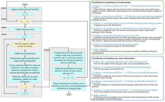
Figure A1.
The simulation process of the graph-theoretic predictive method.
Figure A1.
The simulation process of the graph-theoretic predictive method.
References
- Lv, S.; Wei, Z.; Sun, G.; Chen, S.; Zang, H. Power and traffic nexus: From perspective of power transmission network and electrified highway network. IEEE Trans. Transp. Electrif. 2021, 7, 566–577. [Google Scholar] [CrossRef]
- Hossain, S.; Rokonuzzaman, M.; Rahman, K.S.; Habib, A.K.M.A.; Tan, W.-S.; Mahmud, M.; Chowdhury, S.; Channumsin, S. Grid-Vehicle-Grid (G2V2G) Efficient Power Transmission: An Overview of Concept, Operations, Benefits, Concerns, and Future Challenges. Sustainability 2023, 15, 5782. [Google Scholar] [CrossRef]
- Huang, X.; Wu, D.; Boulet, B. Metaprobformer for charging load probabilistic forecasting of electric vehicle charging stations. IEEE Trans. Intell. Transp. Syst. 2023, 24, 10445–10455. [Google Scholar] [CrossRef]
- Zhao, Z.; Lee, C.K.M.; Ren, J. A two-level charging scheduling method for public electric vehicle charging stations considering heterogeneous demand and nonlinear charging profile. Appl. Energy 2024, 355, 122278. [Google Scholar] [CrossRef]
- He, C.; Zhu, J.; Lan, J.; Li, S.; Wu, W.; Zhu, H. Optimal planning of electric vehicle battery centralized charging station based on EV Load forecasting. IEEE Trans. Ind. Appl. 2022, 58, 6557–6575. [Google Scholar] [CrossRef]
- Sadhukhan, A.; Ahmad, M.S.; Sivasubramani, S. Optimal allocation of EV charging stations in a radial distribution network using probabilistic load modeling. IEEE Trans. Intell. Transp. Syst. 2022, 23, 11376–11385. [Google Scholar] [CrossRef]
- Liu, S.; Fang, C.; Jia, S.; Xiang, Y.; Yang, J. Hierarchical and distributed optimization of distribution network considering spatial and temporal distribution of electric vehicle charging load. Energy Rep. 2023, 9, 308–322. [Google Scholar] [CrossRef]
- Cui, Y.; Hu, Z.; Duan, X. Optimal pricing of public electric vehicle charging stations considering operations of coupled transportation and power systems. IEEE Trans. Smart Grid 2021, 12, 3278–3288. [Google Scholar] [CrossRef]
- Wang, X.; Nie, Y.; Cheng, K.-W.E. Distribution system planning considering stochastic EV penetration and V2G behavior. IEEE Trans. Intell. Transp. Syst. 2020, 21, 149–158. [Google Scholar] [CrossRef]
- Han, X.; Wei, Z.; Hong, Z.; Zhao, S. Ordered charge control considering the uncertainty of charging load of electric vehicles based on Markov chain. Renew. Energy 2020, 161, 419–434. [Google Scholar] [CrossRef]
- Wang, Q.; Yang, X.; Yu, X.; Yun, J.; Zhang, J. Electric Vehicle Participation in Regional Grid Demand Response: Potential Analysis Model and Architecture Planning. Sustainability 2023, 15, 2763. [Google Scholar] [CrossRef]
- Liu, K.; Liu, Y. Stochastic user equilibrium based spatial-temporal distribution prediction of electric vehicle charging load. Appl. Energy 2023, 339, 120943. [Google Scholar] [CrossRef]
- Li, C.; Liao, Y.; Sun, R. Prediction of EV charging load using two-stage time series decomposition and DeepBiLSTM model. IEEE Access 2023, 11, 72925–72941. [Google Scholar] [CrossRef]
- Zhao, Y.; Wang, Z.; Shen, Z. Data-driven framework for large-scale prediction of charging energy in electric vehicles. Appl. Energy 2021, 282 Pt B, 116175. [Google Scholar] [CrossRef]
- Dokur, E.; Erdogan, N.; Kucuksari, S. EV fleet charging load forecasting based on multiple decomposition with CEEMDAN and swarm decomposition. IEEE Access 2022, 10, 62330–62340. [Google Scholar] [CrossRef]
- Zhang, X.; Chan, K.; Li, H. Deep-Learning-Based probabilistic forecasting of electric vehicle charging load with a novel queuing model. IEEE Trans. Cybern. 2021, 51, 3157–3170. [Google Scholar] [CrossRef]
- Zhang, T.; Huang, Y.; Liao, H.; Liang, Y. A hybrid electric vehicle load classification and forecasting approach based on GBDT algorithm and temporal convolutional network. Appl. Energy 2023, 351, 121768. [Google Scholar] [CrossRef]
- Khan, W.; Somers, W.; Walker, S.; de Bont, K.; Van der Velden, J.; Zeiler, W. Comparison of electric vehicle load forecasting across different spatial levels with incorporated uncertainty estimation. Energy 2023, 283, 129213. [Google Scholar] [CrossRef]
- Cao, Y.; Tang, S.; Li, C.; Zhang, P.; Tan, Y.; Zhang, Z.; Li, J. An optimized EV charging model considering TOU price and SOC curve. IEEE Trans. Smart Grid 2012, 3, 388–393. [Google Scholar] [CrossRef]
- Qian, K.; Zhou, C.; Allan, M.; Yuan, Y. Modeling of load demand due to EV battery charging in distribution systems. IEEE Trans. Power Syst. 2011, 26, 802–810. [Google Scholar] [CrossRef]
- Wu, S.; Pang, A. Optimal scheduling strategy for orderly charging and discharging of electric vehicles based on spatio-temporal characteristics. J. Clean. Prod. 2023, 392, 136318. [Google Scholar] [CrossRef]
- Rathor, S.; Saxena, D.; Khadkikar, V. Electric vehicle trip chain information-based hierarchical stochastic energy management with multiple uncertainties. IEEE Trans. Intell. Transp. Syst. 2022, 23, 18492–18501. [Google Scholar] [CrossRef]
- Bian, H.; Guo, Z.; Zhou, C.; Wang, X.; Peng, S.; Zhang, X. Research on orderly charge and discharge strategy of EV based on QPSO algorithm. IEEE Access 2022, 10, 66430–66448. [Google Scholar] [CrossRef]
- Liang, H.; Lee, Z.; Li, G. A calculation model of charge and discharge capacity of electric vehicle cluster based on trip chain. IEEE Access 2020, 8, 142026–142042. [Google Scholar] [CrossRef]
- Tang, D.; Wang, P. Probabilistic modeling of nodal charging demand based on spatial-temporal dynamics of moving electric vehicles. IEEE Trans. Smart Grid 2016, 7, 627–636. [Google Scholar] [CrossRef]
- Cheng, S.; Wei, Z.; Shang, D.; Zhao, Z.; Chen, H. Charging load prediction and distribution network reliability evaluation considering electric vehicles’ spatial-temporal transfer randomness. IEEE Access 2020, 8, 124084–124096. [Google Scholar] [CrossRef]
- Yan, J.; Zhang, J.; Liu, Y.; Lv, G.; Han, S.; Alfonzo, I.E.G. EV charging load simulation and forecasting considering traffic jam and weather to support the integration of renewables and EVs. Renew. Energy 2020, 159, 623–641. [Google Scholar] [CrossRef]
- Guo, Z.; Bian, H.; Zhou, C.; Ren, Q.; Gao, Y. An electric vehicle charging load prediction model for different functional areas based on multithreaded acceleration. J. Energy Storage 2023, 73 Pt A, 108921. [Google Scholar] [CrossRef]
- Shi, X.; Xu, Y.; Guo, Q.; Sun, H.; Gu, W. A distributed EV navigation strategy considering the interaction between power system and traffic network. IEEE Trans. Smart Grid 2020, 11, 3545–3557. [Google Scholar] [CrossRef]
- Long, X.; Yang, J.; Wu, F.; Zhan, X.; Lin, Y.; Xu, J. Prediction of electric vehicle charging load considering interaction between road network and power grid and user’s psychology. Autom. Electr. Power Syst. 2020, 44, 86–93. [Google Scholar] [CrossRef]
- U.S. Department of Transportation, Federal Highway Administration. 2017 National Household Travel Survey. Available online: http://nhts.ornl.gov (accessed on 29 April 2019).
- Pareschi, G.; Küng, L.; Georges, G.; Boulouchos, K. Are travel surveys a good basis for EV models? Validation of simulated charging profiles against empirical data. Appl. Energy 2020, 275, 115318. [Google Scholar] [CrossRef]
- Yang, L.; Shen, Q.; Li, Z. Comparing travel mode and trip chain choices between holidays and weekdays. Transp. Res. Part A Policy Pract. 2016, 91, 273–285. [Google Scholar] [CrossRef]
- Wang, Y.; Zhou, L.; Lv, Y. Lane changing rules based on cellular automation traffic flow model. China J. Highw. Transp. 2008, 89, 89–93. [Google Scholar] [CrossRef]
- TRB. Highway Capacity Manual; TRB: Washington, DC, USA, 1985. [Google Scholar]
- Tu, Q.; Cheng, L.; Yuan, T.; Cheng, Y.; Li, M. The constrained reliable shortest path problem for electric vehicles in the urban transportation network. J. Clean. Prod. 2020, 261, 121130. [Google Scholar] [CrossRef]
- Åkerblom, N.; Chen, Y.; Chehreghani, M.H. Online learning of energy consumption for navigation of electric vehicles. Artif. Intell. 2023, 317, 103879. [Google Scholar] [CrossRef]
- Yuan, Q.; Ye, Y.; Tang, Y.; Liu, X.; Tian, Q. Low carbon electric vehicle charging coordination in coupled transportation and power networks. IEEE Trans. Ind. Appl. 2023, 59, 2162–2172. [Google Scholar] [CrossRef]
- Zhong, J.; Liu, J.; Zhang, X. Charging navigation strategy for electric vehicles considering empty-loading ratio and dynamic electricity price. Sustain. Energy Grids Netw. 2023, 34, 100987. [Google Scholar] [CrossRef]
- Chen, M.; Li, F.; Lin, Q. Random regret minimization model for variable destination-oriented path planning. IEEE Access 2020, 8, 163646–163659. [Google Scholar] [CrossRef]
- Zhang, A.; Zhang, Y.; Liu, Y. Low-carbon cold-chain logistics path optimization problem considering the influence of road impedance. IEEE Access 2023, 11, 124055–124067. [Google Scholar] [CrossRef]
- Lu, L.; Su, T.; Gao, Y.; Qin, F.; Pan, M. FCDT-IWBOA-LSSVR: An innovative hybrid machine learning approach for efficient prediction of short-to-mid-term photovoltaic generation. J. Clean. Prod. 2023, 385, 135716. [Google Scholar] [CrossRef]

Disclaimer/Publisher’s Note: The statements, opinions and data contained in all publications are solely those of the individual author(s) and contributor(s) and not of MDPI and/or the editor(s). MDPI and/or the editor(s) disclaim responsibility for any injury to people or property resulting from any ideas, methods, instructions or products referred to in the content. |
© 2024 by the authors. Licensee MDPI, Basel, Switzerland. This article is an open access article distributed under the terms and conditions of the Creative Commons Attribution (CC BY) license (https://creativecommons.org/licenses/by/4.0/).