Abstract
With the high proportion of renewable energy sources and power electronic devices accessed in the distribution network, the harmonic pollution problem has become increasingly serious. The traditional centralized harmonic mitigation strategy has difficulty in effectively dealing with these scattered and random harmonics. Therefore, a distributed harmonic mitigation strategy based on the dynamic points incentive of blockchain communities is proposed in this paper. Firstly, a comprehensive voltage sensitivity partitioning method with harmonic weight differentiation is proposed to realize the reasonable partitioning of each control node and controlled node in the distribution network concerning variability in harmonic components and their distribution. Then, a harmonic mitigation strategy based on the dynamic integral excitation of self-learning algorithms is constructed to promote self-organized optimization and active distributed coordinated control of mitigation devices. The strategy ensures that the total harmonic voltage distortion rate of each node meets the requirements by adjusting the partitioned collaboration to realize optimal harmonic mitigation. By setting optimized partitions in different scenarios and conducting simulation verification, the results demonstrate the effectiveness of the strategy in this paper. It stimulates synergy between devices through a dynamic incentive mechanism and significantly reduces the total harmonic voltage distortion rate across various test scenarios, reflecting the adaptability of the harmonic mitigation method presented.
1. Introduction
As power electronics continue to advance, mitigation devices are also being updated and modernized, presenting multifunctional, dual-use, active, and other characteristics. The harmonic mitigation device has also surpassed the passive mitigation device to become an active mitigation device [1,2,3]. In recent years, the harmonic problems caused by grid-connected PV have become increasingly serious. The study by Ruiz-Rodriguez et al. [4] presented a new analysis technique that effectively dealt with the interaction between PV harmonic currents and background harmonic voltages, providing a new solution for the harmonic mitigation of distributed generation. In contrast, the study by Hernandez et al. [5] explored the harmonic problems caused by PV systems in an unbalanced network environment by modeling the interaction between the background harmonic voltage and the PV harmonic current. To cope with the high penetration of distributed power supply and the power electrification of source–network–load devices in the distribution network, it is urgent to establish a reasonable and practical distributed mitigation system, make full use of existing resources, reasonably allocate the available capacity of a mitigation device, ensure that the mitigation device plays its role to the maximum extent, and highlight the active characteristics of the current mitigation device.
Harmonic sources within distribution networks are currently distributed throughout the entire network, resulting in a large number of harmonic sources. The efficiency of point-to-point mitigation is suboptimal, and its economic viability could be improved. Consequently, scholars have explored harmonic mitigation devices capable of decentralized mitigation across the entire network, notably Voltage Detection Active Power Filters (VDAPFs) [6,7]. Research [8,9] suggests that installing a VDAPF at feeder ends effectively suppresses harmonic voltage propagation. Building upon this, Ref. [10] proposed a frequency division mitigation-based approach to determine optimal VDAPF placement, demonstrating the efficiency of installing VDAPFs beyond transmission line endpoints.
Other studies [11,12,13,14] have also investigated coordinated mitigation strategies employing multiple VDAPFs to address distributed harmonic pollution in distribution networks. In the study [15], a VDAPF was used as the harmonic mitigation device, and a combination of global optimization with local partition mitigation was adopted to realize harmonic distributed collaborative mitigation. On this basis, the authors of [16] studied multiple VDAPF-coordinated mitigation strategies with automatic gain adjustment. These findings underscore the VDAPF’s suitability for distributed mitigation systems and its pivotal role in distributed harmonic mitigation. This paper will use VDAPF as a mitigation device to study the distributed harmonic mitigation system further.
In harmonic mitigation, studies [17,18] have refined the optimization model for the location and capacity of Active Power Filters (APFs) by employing the grey wolf optimization method and its adaptive algorithm for problem-solving. Through example analyses, it has been verified that the greater the load, the greater the APF mitigation capacity required. In order to make the results accurate and perfect, only load harmonics can be considered. Reference [19] addressed the uncertainty in harmonic pollution in the power grid by developing a multi-objective optimization model. This model aims to minimize filter installation costs and network losses, reduce total harmonic distortion rates in the network, and lower the total demand current distortion rate by employing a trade-off risk analysis method to determine the optimal installation location and capacity for APF. Further, in [20], the economic aspects of APF deployment were explored by introducing a hybrid intelligent algorithm that combined fuzzy logic with the imperialist competitive algorithm to minimize the sum of fixed and variable costs. The feasibility of the hybrid intelligent algorithm was verified by comparing and analyzing the hybrid intelligent algorithm with intelligent algorithms such as particle swarm optimization and harmonious search.
The study of distributed systems is a significant focus of computer science. However, as energy transformation and smart grid technologies continue to evolve, there has been a growing interest in researching distributed mitigation systems within the power sector. Reference [21] introduced blockchain technology into the energy trading system. Using smart contracts, a microgrid peer-to-peer (P2P) trading model, which can meet the needs of professional consumers, was proposed. This model solved the limitations of the traditional centralized energy trading structure and enhanced the utilization of renewable energy.
The energy blockchain consensus mechanism proposed in this paper also provides a reference for the research on the consensus of mitigation devices in the harmonic mitigation system. Reference [22] proposed a multi-region optimal power flow allocation algorithm based on the blockchain consensus mechanism to address the problem that participants in a distributed operating system do not follow the optimization of the specified outputs, which in turn destroys the global optimum. Furthermore, in microgrid transaction settlements [23], Distributed Generators (DGs) utilize color coins instead of transaction power for client transactions. Using the idea of combining distributed mitigation systems and blockchain, when harmonic mitigation devices play the role of a miner in blockchain and equate mining behavior with active mitigation behavior, the self-organized distributed optimization of mitigation devices can be realized.
This paper constructs a distributed harmonic mitigation system based on community thinking. It decentralizes the initial computational resources in the mitigation center and distributes them to various regions. Mitigation devices perform a job similar to miners mining in a blockchain without optimizing the mitigation nodes for centralized mitigation. In a fully distributed context, harmonics are spontaneously and actively coordinated by the mitigation devices in the region by partitioning them with integrated sensitivity as a metric.
The main contributions of this paper are as follows:
- (1)
- A harmonic mitigation strategy based on blockchain community thinking is proposed for the harmonic mitigation problem in distributed networks. The strategy utilizes blockchain technology to construct an incentive mechanism for voltage adjustment devices, thus realizing self-optimization and active distributed coordination among devices, providing an effective solution to the problem of decentralized harmonic sources.
- (2)
- A division mitigation strategy based on comprehensive sensitivity analysis is proposed to enhance the accuracy and efficiency of harmonic mitigation. By assigning weights to different harmonics and dividing them into zones, a more precise area allocation is achieved, ensuring that each mitigation node is allocated to the VDAPF zone with the highest mitigation capability.
- (3)
- A harmonic mitigation strategy based on the dynamic integral excitation of the self-learning algorithm is proposed. The model accurately calculates the number of mitigation points by quantitatively assessing the contribution and performance of the mitigation devices and adopting a self-learning algorithm. At the same time, it stimulates the devices to actively participate in the mitigation task through the dynamic incentive points mechanism, which ensures the fairness and transparency of the calculation process and significantly improves the efficiency and effectiveness of the real-time data analysis and the interference power processing.
This paper is structured as follows. Section 2 proposes the construction of a distributed harmonic mitigation system using blockchain technology to optimize computational resource allocation and improve system efficiency. Section 3 proposes an integrated voltage sensitivity partitioning method with harmonic weight differentiation to realize a reasonable partitioning of each controlled node and control node in the distribution network. Section 4 proposes a harmonic mitigation strategy based on the dynamic integral excitation of the self-learning algorithm to ensure that the system achieves optimal harmonic mitigation under Nash equilibrium. Section 5 validates the effectiveness of the proposed strategy through example simulations, demonstrating the system’s ability to achieve optimal mitigation results under various scenarios. This paper concludes with Section 6, which provides a summary of the main contributions and the significance of this research to enhancing power system efficiency and transparency.
2. Construction of a Distributed Harmonic Mitigation System
Distributed mitigation systems can utilize blockchain [24] technology and smart contracts to achieve distributed mitigation and collaborative decision-making, thereby enhancing the mitigation efficiency and transparency of the power system. Currently, most of the literature on the distributed mitigation of harmonics in distribution networks uses a combination of distributed mitigation and centralized optimization. However, as the number of nodes increases, the computational power required for centralized optimization also increases. In addition, different regions require different sampling periods, and collecting data from each node challenges the system’s real-time performance.
Therefore, to share the computational burden and transform centralized computational power into distributed computational power, this chapter establishes a harmonic distributed mitigation system in the context of harmonic mitigation combined with community thinking.
2.1. Construction of an Active Distributed Harmonic Mitigation System
2.1.1. Blockchain Community Thinking
From the perspective of each region, zonal mitigation is used to mitigate harmonic voltages at the nodes through mitigation devices, and the regions are aligned in their mitigation goals. The current partitioning approach ensures high sensitivity between the internal mitigation nodes and the mitigation nodes in each region while communication links exist among the regions. However, central mitigation with centralized optimization is usually used to achieve overall optimal operation, and then commands are distributed to individual nodes in the system. In the inter-regional collaborative mitigation mode, the mitigation devices in each region must mitigate not only the mitigation nodes in their responsible regions but also the global harmonic voltages.
Given the consistency in mitigation goals in each zone and the decentralized nature of zonal mitigation, community thinking can be applied to harmonic distributed mitigation systems. The decentralized harmonic mitigation model constructed using blockchain distributed thinking differs from the traditional distributed VDAPF, which relies on centralized mitigation for centralized optimization on long-time scales and is adjusted by each zonal VDAPF on short-time scales. In this decentralized model, each mitigation device node participates in the division of labor and cooperation as an independent individual and plays the role of a miner in the blockchain. Under the impetus of the incentive mode, it spontaneously and actively undertakes the mitigation task.
From the perspective of each region, zonal mitigation is used to mitigate harmonic voltages at the nodes through the mitigation device, and the regions are aligned in their mitigation goals. The current partitioning approach ensures high sensitivity between the internal mitigation nodes and the mitigation nodes in each region while communication links exist among the regions. However, a centralized mitigation approach with centralized optimization is often used to achieve an overall optimized operation, with commands distributed to the regions.
2.1.2. A Fit Analysis of the Harmonic Distributed Mitigation System and Blockchain Technology
The distributed mitigation system and the blockchain system are compatible in three core aspects, as shown in Table 1, and are consistent in data disclosure, example integration, and value mining.

Table 1.
Comparison of the distributed mitigation system and the blockchain system.
Data disclosure: In a blockchain, information is tagged in space and time, packaged and transmitted from one block to another, and replicated and propagated to all network nodes in an infinite set, thus making information ubiquitous [25]. In distributed mitigation systems, harmonic voltages are also naturally distributed. Public among nodes, i.e., any node of a distributed mitigation system within a particular region, can exchange information and learn about voltage variations in other nodes so that the remaining capacity of the mitigation device of the mitigation nodes at a given moment can be known among neighboring regions.
Arithmetic Integration: Through miners mining to obtain rewards, the blockchain splits the problem that requires substantial arithmetic power to be solved into many small parts and then distributes them to computer terminals for processing through distributed arithmetic integration. In the distributed mitigation system, each mitigation device plays the role of a miner in the blockchain, actively assisting neighboring regions in collaborative mitigation while managing harmonic voltages in its area and reasonably allocating its remaining capacity. Each mitigation device aims to achieve the best mitigation effect, and its total computing power far exceeds the centralized optimization of the central controller. Each mitigation device has the initiative to realize community co-mitigation within the system.
Value Mining: A blockchain can reconfigure resources to create new value, thus activating the potential value of idle resources from the supply-side perspective, effectively enhancing resource utilization and matching the supply and demand of social resources. In distributed mitigation, zoning is performed only through sensitivity. When facing uncertain harmonic disturbances and harmonic pollution on a long-term scale, there may be a situation in which the mitigation capacity of individual regions needs to be improved. In contrast, other mitigation devices still have spare capacity. In this case, by reallocating the remaining capacity and redistributing the attribution of the controlled nodes, it is possible to ensure that none of the remaining capacity is wasted and that all regions can achieve the mitigation objectives.
2.2. Integral Design for Mitigation Systems
This paper establishes a reasonable and open incentive and punishment mechanism to make the mitigation device actively participate in mitigation within the system. Quantifying the mitigation effect of the mitigation device and converting it into local digital assets is an essential part of the smooth realization of the above mechanism. To a large extent, the blockchain can digitize assets and expand the circulation of digital assets, thus breaking through the boundaries of previous digital assets. For example, the existing Bitcoin transaction is considered the best application scenario for current blockchain technology, mainly because of the blockchain’s strong guarantee of the existence and authenticity of digital assets, making it possible for digital assets to circulate on a large scale.
To this end, this paper designs a mitigation integral to measure the digital assets of each mitigation device. As a token, such integral mitigation has the characteristics of limited circulation; that is, it is only used in a restricted range of distributed mitigation systems [26]. Therefore, a private chain with mitigation read and write permissions is used to circulate the mitigation integral. The mitigation performance of the corresponding mitigation device determines the mitigation score. If the mitigation behavior improves the mitigation effect of the nearby area, the corresponding mitigation score increases; otherwise, it decreases. The specific calculation method of the mitigation integral will be introduced in detail in the third section of this paper. The circulation of mitigation points mainly includes incentive generation, present value exchange, and chain transaction.
2.3. Local Communication Network Connection of the Distributed Mitigation System
The distributed mitigation system divides the distribution network into different regions. Each region has a mitigation device, namely, a VDAPF, but each partition is not isolated. In the distributed mitigation system, the nodes where each mitigation device is located will communicate with each other to cope with the uncertainty in harmonic pollution. When a regional node’s harmonic voltage distortion rate exceeds the limit, the adjacent area can assist in mitigation. At this time, communication connections between the partitions are required.
Therefore, a two-way communication connection is set between the VDAPFs in each region. Each region can exchange information in time, and two-way communication has higher reliability, avoiding the one-way communication line fault disconnecting a region from the other areas. When there is a sizeable harmonic disturbance, it is impossible to accept the assistance of adjacent areas. Figure 1 illustrates the blockchain-based harmonic pollution monitoring and mitigation process, highlighting its key role in data management and decentralized coordination.

Figure 1.
Blockchain-based harmonic mitigation flowchart.
The distribution network is represented by a graph model , and the communication connection topology between each VDAPF can be intuitively understood through Figure 2. represents the set of vertices of each VDAPF. is the edges connected by vertices, , where and are unequal. represents the adjacency matrix of . If there are VDAPFs, then is an -order square matrix. The corresponding values of each element in the matrix are obtained according to Formula (1).
Figure 2.
VDAPF communication connection topology diagram.
In this paper, five VDAPFs are configured, that is, = 5 in the above. If the connection of the vertices where the mitigation device is located as shown in Figure 2, the adjacency matrix representing the relationship between can be obtained as
The degree matrix of is a diagonal matrix. Each element on the diagonal of the matrix represents the degree of the vertex . The value of is the sum of the edges associated with the vertex . In order to make the communication between each VDAPF more reliable, this paper ensures that the device can communicate directly in both directions, so the degree matrix is
3. Partition Mitigation Strategy Based on Comprehensive Sensitivity Analysis
3.1. Analysis of the VDAPF Principle
The structural principle of VDAPFs is shown in Figure 3. To satisfy the grid-side harmonic mitigation requirements, the VDAPF is connected in parallel with the grid bus. When a harmonic voltage input is detected at the access point, the APF converter is mitigated to output a harmonic compensation current to suppress the voltage distortion of its access point. From an external perspective, this is equivalent to a virtual conductance path parallel to the access point, which can effectively release the harmonic current.
Figure 3.
Structure diagram of VDAPF.
From Figure 3, it can be seen that the VDAPF mainly realizes the harmonic mitigation function through the steps of harmonic voltage detection, command current arithmetic, inverter direct AC conversion, and current tracking control. The blue dashed box indicates the control section of the VDAPF. First, the harmonic voltage detection module detects the harmonic components in the grid voltage in real time and outputs the harmonic voltage signal . Then, the required harmonic current command is calculated by the command current calculation module based on the harmonic voltage signal . The current tracking control module compares the actual current with the command current to generate the control signal . The DC voltage control module maintains the stability of the DC side voltage . Ultimately, the control signal is converted into a switching signal through the PWM controller to regulate the output of the compensation current, thereby suppressing the voltage harmonics at the point of connection. Figure 4 shows a schematic diagram of the operating principle of the VDAPF, from which it can be seen that the VDAPF converts the detected harmonic voltage into a current command by introducing a control gain , that is .
Figure 4.
The working principle of VDAPFs.
3.2. A Partition Method Based on Sensitivity Analysis
3.2.1. Sensitivity Analysis
The root cause of harmonic mitigation is traced. Taking a VDAPF as an example, according to its external characteristics, the greater the virtual harmonic conductance, the easier it is to achieve the expected mitigation effect.
Hence, the increment in the mitigation conductance of the adjustable harmonic voltage filter (VDAPF) has a decisive influence on the harmonic voltage suppression effect at each control node, which determines the effectiveness of the harmonic mitigation in the whole area. For h-order harmonics, the partial derivative of the harmonic voltage at any control node to the harmonic mitigation conductance at the control node is defined as the sensitivity , and the specific expression is given in Formula (4).
where is the -times harmonic voltage of the mitigation node ; is the equivalent conductance of the mitigation node; and represents the degree of change in the harmonic voltage of the mitigation node caused by the conductance change of the mitigation node .
The sensitivity can be derived from the harmonic propagation equation. The harmonic power flow equation constraints [27] are shown in Formula (5).
where and are the column vectors of node harmonic voltage and node injected harmonic current, respectively, and is the harmonic admittance matrix determined by the system network parameters.
The equivalent conductance of the mitigation node exists in the diagonal element of , and Formula (5) is expanded, as shown in Formula (6).
where of the controlling node is the equivalent conductance of node accessing the VDAPF, and = 0 of the controlled node; is the portion of the self-conductance of node after removing . Since is the predicted quantity, is the network parameter constant, and is the dependent variable determined by . The relationship between the voltage of each node and the conductance of the controlled node can be expressed in the form of Formula (6). Taking the optimal conductance value of each VDAPF obtained from the global optimization as a benchmark, the value of , the sensitivity of to , can be found for Formula (6).
3.2.2. Comprehensive Sensitivity Analysis
To divide the region, the method of finding the mitigation node by the mitigation node is adopted. The more sensitive the response of the mitigation node voltage to the change in the mitigation node harmonic is, the stronger the mitigation node has mitigation over the mitigation node. Therefore, comparing the voltage sensitivity between each mitigation node and each mitigation node , each mitigation node is divided into the area where the mitigation node has the largest mitigation.
Considering the varying proportions of each harmonic within the power grid, the weighted setting of each harmonic is carried out, and the regional division is carried out through comprehensive harmonic sensitivity to accurately determine the partition results. The comprehensive sensitivity is calculated as Formula (7).
where is the weighting coefficient corresponding to the h-harmonics. The specific value of the weighting coefficient can be determined by the method of the superior order diagram.
In the system, there are controlling nodes and controlled nodes. By applying Formulas (4)–(7), the integrated sensitivity matrix, denoted as , can be derived.
The maximum value of each column vector is found by Equation (8), and the corresponding to the maximum value angle is the node where the mitigation node belongs to the mitigation device. The initial partition meticulously separates the distribution network into regions.
3.3. Observation Node Selection
In this paper, some nodes in each region are selected as observation nodes through a particular proportion, and the voltage distortion rate of the observation nodes is used to judge whether the harmonic voltage of the whole network meets the standard [28].
In order to improve the accuracy of the observation results, this study requires significant interconnections among the observed nodes and other nodes. Based on the sensitivity mentioned earlier in the analysis method, we define the strength of the influence of the harmonic voltage of node on the harmonic voltage of node as the harmonic voltage coupling degree. For h-order harmonics, the coupling degree between node and node can be calculated by Formula (9).
Considering that the voltage coupling between nodes varies because of different harmonic frequencies, the integrated harmonic voltage coupling of any two nodes and is obtained by seeking the root mean square of the harmonic voltage coupling between nodes, as in Formula (10).
where Π is the total number of harmonic numbers considered, and H is the highest harmonic number.
A flowchart of node clustering method is shown in Figure 5.
Figure 5.
Clustering algorithm flowchart.
The K-mean clustering algorithm is known for its efficient computational performance and simplicity of principles, so it is chosen for data clustering in this study. In this framework, we define the inverse of the integrated coupling of harmonic voltages among nodes as the electrical distance to quantify the interrelationships among nodes. The details are shown in Formula (11).
4. A Harmonic Mitigation Strategy Based on Dynamic Integral Excitation of Self-Learning Algorithms
4.1. Harmonic Mitigation Incentive Model
4.1.1. Mitigation Integral Calculation Method
In this paper, the mitigation device’s mitigation contribution and mitigation performance are quantified by mitigation integral. Therefore, the calculation method of the performance factor is determined by considering the overall mitigation effect of the distributed system and the individual mitigation performance of each mitigation device.
In order to assess the harmonic mitigation effectiveness of the system comprehensively, the total distortion of the node voltage of the whole system is used as a measure. This index reflects the system’s performance in terms of harmonic mitigation, where the lower the total node voltage distortion, the better the system’s mitigation effect. Therefore, the global effect factor of the system at the time for assisted mitigation can be calculated according to Formula (12).
where is the sum of the harmonic voltage distortion rates weighted at all nodes of the system [29,30], while denotes the maximum permissible value of the sum of the harmonic voltage distortion rates weighted at all nodes of the system, i.e., the distortion rate corresponding to the minimum standard of the qualified voltage quality. In order to ensure the power quality of the distributed mitigation system, it is necessary to satisfy that the value of is less than or equal to the value of is constant, from which it can be inferred that the value of will be in the range of [0, 1]. Specifically, the formula for is shown in Equation (13).
where is the total number of nodes in the distributed mitigation system; is the weight set according to the different nodes on the differentiated demand for harmonic levels, as shown in Formula (14), which can be obtained by the sensitivity factor ; and characterizes the degree of node on the requirements of the voltage distortion, where the node connected to the load has more stringent voltage distortion requirements the greater the value of . Therefore, serves as the sensitivity factor for controlled node , with its value derived from the highest harmonic tolerance level of the device connected to the node. Meanwhile, represents the total voltage distortion rate of controlled node , as defined in Formula (15).
where represents the effective value of node for h-order harmonic voltage, which can be obtained by the power flow calculation of h-order harmonics; represents the fundamental voltage effective value of node .
The individual mitigation performance of the mitigation device can be quantified in the form of a ratio based on its spontaneous compensation capacity combined with the positive degree. The individual performance factor of the assisted mitigation device is shown in Formula (16).
where is the number of VDAPFs involved in assisting the mitigation process; is the positive degree of mitigation device participating in assisting mitigation, which is within the range of [0, 1]; and , , and are the actual compensation capacity of the VDAPF before assisted mitigation, the actual compensation capacity, and the rated capacity after assisted mitigation [31].
The actual compensation capacity of the VDAPF can be obtained by Formula (17).
where is the hth harmonic conductance of the VDAPF at the mitigation node and is the hth harmonic voltage of node .
The actual harmonic mitigation capacity of the VDAPF needs to meet the capacity limit requirements, and the constraint is:
In summary, this paper comprehensively considers the two indicators of the overall mitigation effect and the individual mitigation performance of each mitigation device. It gives the calculation method of the VDAPF performance factor of the station under the assisted mitigation as the judgment basis for the mitigation performance of each harmonic mitigation device, as shown in Formula (19).
where is the weight coefficient, and the value is [0, 1]. It can be seen that the greater the , the more the mitigation integral focuses on the consideration of the mitigation effect; otherwise, more emphasis is placed on the individual mitigation performance of mitigation device. For a piece of a specific mitigation device, when the mitigation system selects a larger , it can only bring more minor benefits because of the high contribution rate of the individual’s assistance in mitigation, which will lead to a decrease in the active mitigation of the mitigation device, that is, and are negatively correlated. Assume that the two are linear, as shown in Formula (20).
where represents the positive coefficient of the specific mitigation device. Because is in the range of [0, 1], the value of is also in the range of [0, 1]. The positive coefficient of mitigation is affected by the weight coefficient, but the degree of influence of each mitigation device is different; that is, the value of is different.
As the core component of a blockchain, the smart contract has critical code thinking. Intelligent contracts, through absolute machine language execution, automatically execute the contract jointly agreed on by the community members, which can effectively avoid interest strife tampering and other problems. The mitigation points of each mitigation device reflect the attitude and participation in maintaining power quality. They are directly linked to regional interests, so if there are loopholes and trust issues in the point calculation process, it will seriously dampen the enthusiasm of mitigation devices to take the initiative to undertake mitigation tasks. For this reason, the calculation of the above mitigation points is completed by the blockchain smart contract.
4.1.2. Distributed Mitigation System Response
The distributed mitigation system synchronously exchanges information through the communication network between the VDAPFs when it receives an early warning and determines the local operating parameters of each VDAPF. This paper assists the information dissemination and exchange in the mitigation process in the same way as the existing distributed mitigation system in the information dissemination and exchange. The dissemination of harmonic mitigation information does not pass through the blockchain network, and there is no communication delay because of the introduction of the blockchain. The local processors of the VDAPFs can respond to harmonic disturbances in real-time and adjust the harmonic mitigation scheme through the distributed computation of the local processors in each region. The harmonic mitigation scheme is adjusted, and distributed arithmetic power is centralized without waiting for the central controller to perform centralized optimization and then send down the instruction to the local controller, which saves the arithmetic power cost generated by the complex computation and avoids the computation delay to a large extent. The harmonic conductor–harmonic voltage locally controlled upward adjustment characteristic of the VDAPF is shown in Figure 6.
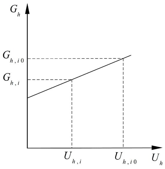
Figure 6.
VDAPF local mitigation G-U upward adjustment characteristics.
In the distributed mitigation system based on community thinking, each mitigation device responds to harmonic perturbation and undertakes the mitigation task spontaneously and actively by analyzing the operation mechanism of VDAPF to make it better assume the role of a miner. The positivity coefficient is used as the integrated conductance regulation degree of each device, and the harmonic conductance–harmonic voltage uplift characteristic of the VDAPF under the harmonic frequency is expressed as
where and are the initial values of the harmonic command conductance required for the successful participation in assisted mitigation and the harmonic conductance before participation in assisted mitigation of the VDAPF accessed at node , respectively; is the degree of regulation of the harmonic conductance of the VDAPF at this node; and and are the initial value of the pre-adjusted harmonic voltage of node at which the VDAPF is located and the actual adjusted h-harmonic voltage value.
4.2. Assistance Mitigation in Integral Acquisition Based on the Self-Learning Algorithm
The acquisition of the mitigation integral is related to the actual auxiliary compensation capacity and the degree of harmonic voltage mitigation. When the capacity of a particular area is insufficient, the total harmonic voltage distortion of the mitigation node in the area exceeds the limit, and the mitigation device in the adjacent area actively responds and governs the edge node to obtain the assistance mitigation integral. Because the distance between the accessed VDAPF and the mitigation nodes will affect the mitigation effect, the mitigation effect will decrease as the distance increases. Therefore, each assisted area only selects two mitigation devices closest to the edge node for directly assisted mitigation, while the remaining mitigation device directly participating in the mitigation effect of the edge node is weak. The area with edge nodes is indirectly assisted by assisting the area with a qualified distortion rate before co-mitigation, and the principle of proximity between the mitigation device and the mitigation node is also followed. If each mitigation device wants to obtain more points in the distributed mitigation system, it is necessary to constantly adjust its assistance compensation capacity, denoted as , which is limited by the remaining mitigation capacity of the mitigation device. The constraint condition is
where represents the actual assistance compensation. After many training sessions, the mitigation device obtains the harmonic compensation value , where h benefits more points. According to the obtained by training, the compensation is carried out to form the situation where the edge node is governed by one or more devices so that the ownership of the mitigation node changes, and the partition result changes accordingly. However, all the mitigation devices have a common goal to achieve community co-mitigation by obtaining points and finally making the overall situation achieve the best mitigation effect.
The self-learning algorithm refers to the ability to input data to autonomously learn and adjust the weights to improve the prediction and classification accuracy of the data. This paper, on the other hand, uses a self-learning algorithm for training to assist in the mitigation of the compensating capacity value. The specific self-learning algorithm process is as follows:
Firstly, each parameter is initialized, and the best assistance compensation capacity is assigned 0. The optimal integral value is also assigned 0; the optimal number of adjustments is assigned 1; and the step size is set to assist mitigation (compensation capacity change of each output).
Secondly, a reasonable number of training times is set, the remaining mitigation capacity is input, and min(, ) is assigned first to . The objective function is then used to obtain the maximum integral value and find the corresponding auxiliary compensation capacity .The process is repeated until the maximum limit of the remaining capacity is reached.
Thirdly, each time the value of the harmonic compensation capacity is adjusted, by calculating and comparing the score obtained from the latest training with the score remembered from the previous training and the maximum score recorded in the previous training, if the current integral is greater than , the current integral value is assigned to ; otherwise, remains unchanged.
Fourthly, the number of steps of the auxiliary output is determined by the maximum integral , and finally, is also determined.
The VDAPF assists each station in finding the suitable for itself through training. At the initial moment of the assisted mitigation, the active degree of participation is determined by the reference weight coefficient, and the equivalent conductance of the assistance is obtained by calculating Formula (21). The harmonic voltage distortion rate of the edge node is reduced, and the whole system has a better mitigation effect. After the assisted mitigation process ends, the points obtained from this active mitigation will be settled, and the mitigation points of each mitigation device will be refreshed.
4.3. Integral Settlement Process of Distributed Mitigation Systems
The global effect factor is determined by the total distortion rate of the node voltage in the local area, which cannot be maliciously tampered with and can be calculated. In contrast, the individual performance factor of the mitigation device itself is related to the harmonic compensation capacity, which may lead to over-reporting and false reporting. In order to ensure the excellent operation of the distributed mitigation system and the fairness and justice of the integral calculation, the integral settlement process is used, as shown in Figure 7.
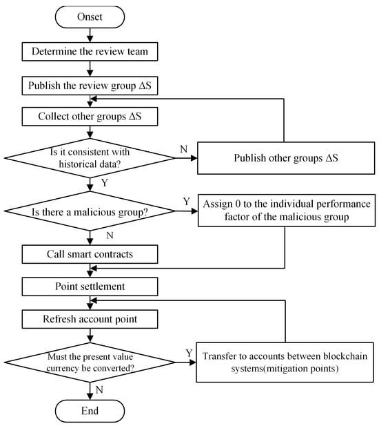
Figure 7.
Point settlement process.
5. Example Simulation and Analysis
5.1. Delineation Results
The IEEE-33 bus system distribution network system is used for example analysis. The harmonic current injection of Scenario 1 and Scenario 2 is shown in Figure A1 and Figure A2 in the Appendix A, respectively.
Taking Scenario 1 as an example, the harmonic current data corresponding to each harmonic in Scenario 1 is input into the SPSSAU system, and the optimal sequence diagram method is used to analyze the weight data. The system calculates the average value of each harmonic and uses the average value to construct the matrix. After data processing, the importance of each harmonic in the corresponding scenario is obtained.
In Table 2, the number 0 is relatively unimportant, the number 1 is relatively more important, and the number 0.5 is equally essential. Compared with the data in the table, the importance of the fifth harmonic in the mitigation system is the highest.
Table 2.
Priority chat weight calculation table.
Dex score TTL is obtained by adding the weight value of each harmonic in each row relative to a particular harmonic in Table 2. For example, the index score TTL5 of the fifth harmonic is 0.5 + 1 + 1 + 1 = 3.5. The TTL of each harmonic is calculated and normalized, and then the specific weight values of the 5th, 7th, 11th, and 13th harmonics in the system are obtained. The calculation results are shown in Table 3.
Table 3.
The weight calculation results of the priority graph.
Figure 8 shows the specific value of each harmonic weight. Combining the obtained harmonic sensitivity weight with the partition method of the comprehensive sensitivity analysis in Section 3, the partition results based on comprehensive sensitivity partition can be obtained and finally divided into five regions Region I–Region V. The partition results are shown in Figure 9.
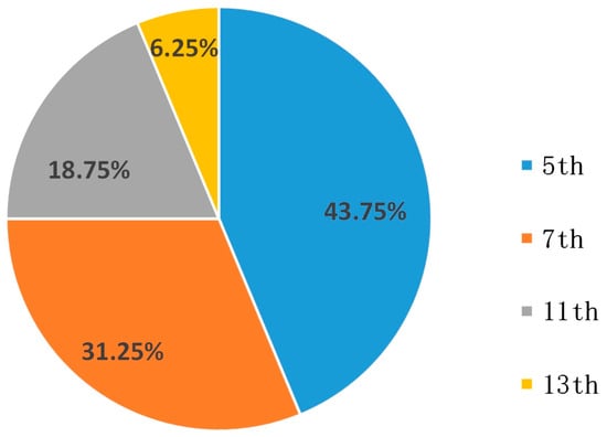
Figure 8.
Each harmonic weight diagram.
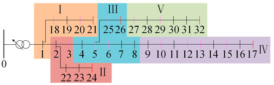
Figure 9.
The partition result diagram based on comprehensive sensitivity analysis of IEEE-33 bus system.
5.2. Observation Node Selection Results
According to the calculation method of observation nodes in Table 3, nodes 18, 20, 3, 24, 5, 6, 25, 10, 12, 13, 15, 27, 29, and 32 are selected as observation nodes, as shown in Table 4.
Table 4.
Selection of observation nodes in each region of IEEE-33 bus system.
5.3. Example Solution
This paper assumes that all five mitigation devices are involved in partition adjustment and regional mutual assistance. Taking the sizeable harmonic pollution in Region III as an example, the mitigation device = 1 in Regions I and II is set. It can be seen from Formula (18) that if takes 1, the mitigation device 1 and the mitigation device 2 do not participate in the auxiliary mitigation process of Region III. Only the VDAPF of Region IV and Region V provide compensation capacity for Region III with edge nodes through direct assistance.
Taking the maximum number of devices participating in assisted mitigation as an example, five mitigation devices are set to participate in 200 self-learning processes. The disturbance of the harmonic mitigation system refers to the harmonic current injection of Scenario 2, and the weight coefficient of the system is 0.5. In the absence of early warning, the time interval of each round of assisted adjustment is one minute. The system will be adjusted in real time when the early warning is received.
During the training process, each mitigation device increases by 0.002 s each time. The growth rate of compensation in the training process is different because of the different enthusiasm of each mitigation device. For example, the of mitigation device 4 is the smallest, so is the largest, which is intuitively reflected in the largest growth slope, as shown in Figure 10. At the same time, if a mitigation device reaches the upper limit of the available compensation capacity during the comigration process, it is compensated according to the maximum compensation capacity, and the compensation capacity of the subsequent training process will not increase again.
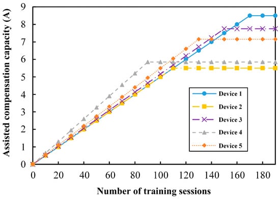
Figure 10.
Each mitigation device assists in compensating capacity in 200 training sessions.
Table 5 shows the specific values of the residual capacity and the coefficient corresponding to each mitigation device.
Table 5.
The residual compensation capacity and positivity factor for each mitigation device of IEEE-33 bus system.
As shown in Figure 11, when the compensation capacity of the mitigation device is adjusted to the capacity required by the adjacent area, the integral increases. During the 70th training session, the points for all mitigation devices peaked. Because the increase in points is a comprehensive consideration of the two factors of the output of the mitigation device and the mitigation effect, when the compensation capacity of the adjacent area continues to increase, it may lead to an insufficient mitigation capacity of the original mitigation area and affect the mitigation effect of the whole area. At this time, the points of all the mitigation devices gradually decline. In the 170th training session, the No.1 mitigation device with the most sufficient remaining mitigation capacity reaches the upper limit. In summary, the mitigation system takes the best training effect at the 70th training session. At this time, the optimal changes in the conductance of the actual mitigation device are 0.36, 0.28, 0.85, 0.59, and 0.63 S, respectively.
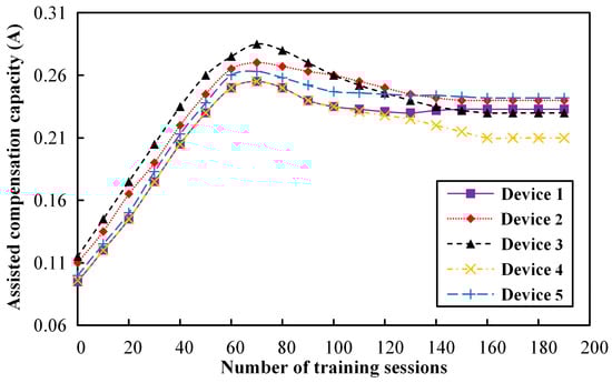
Figure 11.
The integral changes in each mitigation device in 200 trainings of IEEE-33 bus system.
5.4. Comparative Analysis
Relying only on the traditional partitioning method, each VDAPF only governs the harmonic voltage at the mitigation point in the area, and some observation nodes still have a voltage distortion rate exceeding the limit after the partition mitigation under Scenario 2. As shown in Figure 12, when the partition adjustment is carried out according to the best training effect, the harmonic distortion rates of the observation nodes in Scenario 1 and Scenario 2 align with the mitigation standards after the adjacent mitigation device assists in the mitigation. The harmonic distortion rates of some observation nodes in Scenario 2 that are not qualified by the initial partition mitigation are optimized to be below 4%. This proves the rationality of the above partition adjustment results, and the distributed mitigation system can achieve the ideal mitigation effect through the regional mutual assistance model.
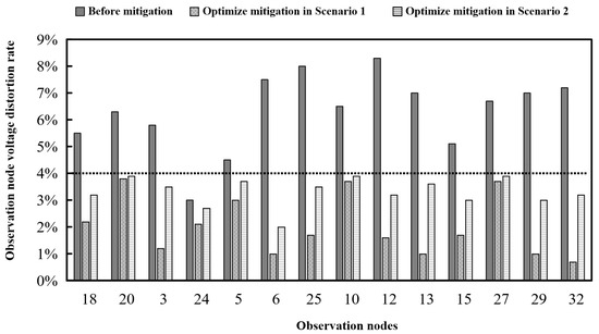
Figure 12.
Comparison of mitigation results after partition optimization in different scenarios.
Compared with decentralized mitigation, as shown in Figure 13, whether it is a slight disturbance or harmonic pollution, the harmonic voltage distortion rate of the observation node after partition adjustment is below 4%, which meets the harmonic voltage mitigation standard. However, there is a situation where the harmonic voltage distortion rate is greater than 4% in decentralized mitigation, which does not meet the standard. To ensure that the voltage distortion rate meets the required standards, augmenting the quantity of mitigation devices is necessary. This approach enhances the mitigation efficacy while concurrently reducing economic costs. It can be seen that reasonable distributed mitigation is superior to decentralized mitigation regarding economy and the mitigation effect.
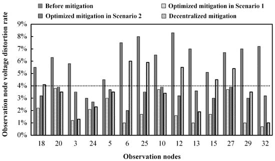
Figure 13.
Comparison of the results of optimized partition mitigation and decentralized mitigation in different scenarios.
Based on the harmonic voltage distortion of the node, the harmonic distortion rate of the mitigation node meets the requirements. For several nodes (nodes 6, 25, and 12) with harmonic distortion rates greater than 7% before mitigation, under the incentive model of this section, the VDAPF obtains integral active mitigation, avoiding the waste of resources and maximizing the value of its residual compensation capacity. After the initial partition mitigation, the harmonic voltage distortion rate of node 25 still decreased from 4.5% to 3.5% after collaborative mitigation, and the mitigation effect improved significantly.
In order to further verify the rationality of the collaborative mitigation scheme, the total harmonic voltage distortion rate of each node in the whole network is used as the evaluation standard of the mitigation effect. The simulation is analyzed and verified in the cases of less harmonic pollution in Scenario 1 and heavier harmonic pollution in Scenario 2. Two different harmonic mitigation methods are compared as follows: method 1, harmonic mitigation by comprehensive sensitivity partition, and method 2, VDAPF active output to assist harmonic co-mitigation in adjacent areas.
Comparing the harmonic mitigation effects of the two methods in two scenarios, the mitigation effect of method 2 is better than that of method 1. As shown in Figure 14, after optimizing the partition mitigation, the of the edge nodes in Scenario 2 is governed below 4%, which meets the mitigation requirements.
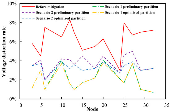
Figure 14.
Comparison of preliminary partition and optimized partition results.
The mitigation effects of the two scenarios are analyzed. Firstly, in Scenario 1, the results of the two mitigation methods are compared, as shown in Figure 15.

Figure 15.
The total voltage distortion rate of each node before and after mitigation in Scenario 1.
Each node’s total harmonic voltage distortion rate is concentrated at about 7% before mitigation. After mitigation by the two methods, most nodes’ total harmonic voltage distortion rates are kept below 3% for even more than half of the nodes. The total harmonic voltage distortion is at a low level of about 2%, and the curve trend of method 1 and method 2 in Figure 15 has a high similarity. This shows that the two methods are applicable in the case of light harmonic pollution, and the distributed mitigation system will not issue an early warning request for regional assistance. It is only necessary to adjust each VDAPF output point by periodic optimization. In Scenario 1, the mitigation nodes in each region can mitigate the harmonic voltage of each node by relying on the VDAPF in the region.
The harmonic voltage distortion rate at nodes 3, 6, 13, and 32 is significantly lower than that before mitigation and lower than the voltage distortion of the other nodes because these nodes are more sensitive to harmonic distortion and have higher requirements for voltage distortion than the other nodes. Therefore, in calculating the global effect factor, the sensitivity factor of the above nodes is given an immense value. Finally, the voltage distortion is globally up to standard, and the harmonic voltage distortion rate required by the sensitive nodes is targeted.
The effect of the two mitigation methods under the harmonic current injected in Scenario 2 is shown in Figure 16. In the case of heavy harmonic pollution in Scenario 2, the voltage distortion rate of multiple nodes in the system exceeds the limit in method 1. In method 2, to prevent node voltage distortion from exceeding the limit, an early warning signal is sent to the whole distributed system in advance, and each VDAPF in the whole network receives the operating position of other VDAPFs at the same time. Figure 5, Figure 6, Figure 7, Figure 8, Figure 9, Figure 10, Figure 11, Figure 12, Figure 13, Figure 14 show each node’s harmonic voltage mitigation results when the system weight coefficient = 0.5; that is, the individual performance of the mitigation device is consistent with the proportion of the global mitigation effect. At this time, the voltage distortion of all nodes is below 4%, which proves the feasibility and superiority of method 2. is set to 0.5 to meet the mitigation requirements of the distributed mitigation system.
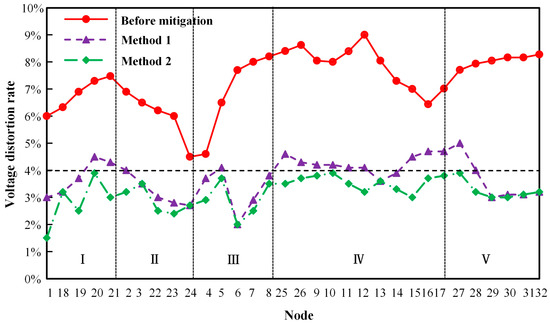
Figure 16.
The total voltage distortion rate of each node before and after mitigation in Scenario 2.
Changing the weight coefficient of the system in the extreme case of = 0 means that only the mitigation performance of the mitigation device is concerned, and the ideal mitigation effect cannot be obtained by providing a large compensation capacity, which does not meet the needs of the global mitigation effect and the system economy. When = 1, only the global mitigation effect is considered, and the enthusiasm of mitigation devices to participate in mitigation is seriously reduced, which does not meet the needs of VDAPF self-organizing distributed optimization. Figure 16 shows that when = 0.5, the system’s harmonic mitigation demand is met. Next, a further discussion is provided on the influence of the harmonic distributed mitigation system as the weight coefficient increases. After setting = 0.8, the harmonic voltage distortion rate after mitigation is obtained for each grid node, as shown in Figure 17.
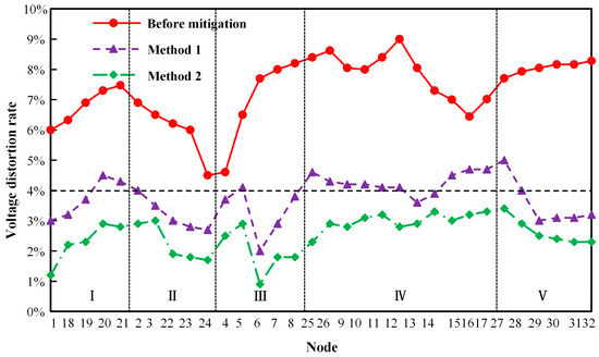
Figure 17.
The total voltage distortion rate of each node before and after mitigation in Scenario 2 when = 0.8.
Compared with the harmonic mitigation effect of each node when = 0.5, the harmonic distortion rate of each node decreases further when = 0.8, and the global harmonic voltage mitigation effect of the latter is better than that of the former. This shows that an appropriate increase in the value can reduce the comprehensive voltage distortion rate of the system and enhance the harmonic mitigation effect of the system. When is in the range of 0.9 to 1, the positive degree of the mitigation device decreases obviously with the increase in , and the total score of the mitigation effect also decreases. Similarly, other values of are verified. When 0.3 ≤ ≤ 0.9, the stability of the distributed mitigation system is better, and the higher requirements of the system on the harmonic distortion rate can be met by adjusting the value of = 0.8.
5.5. IEEE 69 Node Scalability Evaluation Arithmetic Analysis
In this study, the IEEE-69 bus system is used to verify the scalability and applicability of the proposed method further. The simulation example is used to evaluate the effectiveness of the proposed method for harmonic mitigation in larger-scale power systems with different topologies.
The IEEE-69 bus system is divided into six regions based on the integrated sensitivity partitioning method, including Region I–Region VI, as shown in Figure 18. The mitigation nodes and observation nodes selected by the method in Section 4 are listed in Table 6.
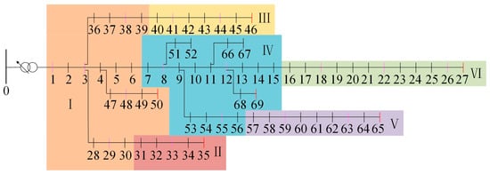
Figure 18.
The partition result diagram based on comprehensive sensitivity analysis of IEEE-69 bus system.
Table 6.
Selection of observation nodes in each region of IEEE-69 bus system.
Based on the partition results of the 69-bus system, six VDAPF harmonic mitigation devices are used to mitigate the harmonics in different regions synergistically. The parameters of the IEEE 69-bus system are consistent with those of the IEEE 33-bus system to verify the adaptability of the proposed method.
Figure 19 illustrates the compensation capacity changes in six mitigation devices with 200 training times in the IEEE 69-bus system experiment. During the training process, the compensation capacity of each mitigation device increases by 0.002 S per training. The growth rate of the compensation capacity varies because of the different positivity values of each device. For example, mitigation device 5 participates in harmonic mitigation with the highest positivity, which is intuitively reflected in the largest growth slope. In addition, although the compensation capacity of device 6 is not the fastest growth, it can ultimately achieve and maintain a high compensation capacity, which is essential to ensure the stable operation of the power system under extreme conditions.
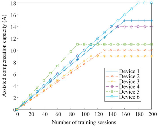
Figure 19.
Compensation capacity assisted by each mitigation device in 200 training sessions of the IEEE 69-bus system.
Table 7 demonstrates the residual compensation capacity of the devices under different nodes and their positivity to assess the performance and participation of each device. Among them, mitigation device 6 at node 27 has the largest residual compensation capacity of 18.0 A and a positivity factor = 0.6. This implies that mitigation device 6 still has great potential in harmonic mitigation, and it is necessary to adjust strategies to improve the positivity of the mitigation device. In contrast, mitigation device 1 at node 50 shows sufficient residual capacity and the highest positivity, indicating that mitigation device 1 fully utilized its potential during the harmonic mitigation process and has satisfactory harmonic mitigation performance.
Table 7.
The residual compensation capacity and positivity factor for each mitigation device of IEEE-69 bus system.
As shown in Figure 20, when the compensation capacity of the mitigation devices is adjusted with the target of the required capacity of the neighboring regions, the mitigation integral of the device increases accordingly. At the 85th training, the mitigation integral of all the mitigation devices reached its peak. However, with the increase in the compensation capacity, the residual capacity of the self-region of the mitigation device may be insufficient, which will affect the effect of the whole area. This indicates that the mitigation integral strategy proposed in this paper can effectively control harmonic mitigation devices for the harmonic collaborative mitigation of the whole system.
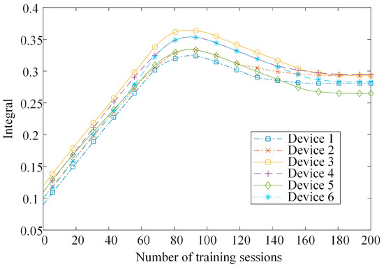
Figure 20.
The integral changes in each mitigation device in 200 trainings of IEEE-69 bus system.
After injecting the harmonic currents of Scenario 1, the total harmonic voltage distortion rates (THDv) of the IEEE 69-bus system are mainly concentrated around 8%, as shown in Figure 21. After the harmonic mitigation by the two methods, the THDv of most nodes is significantly reduced to below 4.5%, indicating that both methods are effective in reducing harmonic pollution. Specifically, method 1 can reduce the THDv of most regions, but there are still some nodes with high THDv, such as nodes 16 and 17. On the other hand, method 2 can significantly reduce the THDv of most nodes in all regions, indicating that method 2 has a better harmonic mitigation effect.
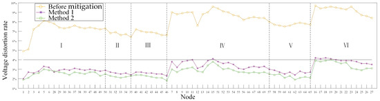
Figure 21.
Total harmonic voltage distortion rate of each node before and after mitigation in Scenario 1.
Figure 22 demonstrates the effectiveness of harmonic mitigation with the system weighting factor under the condition of heavy harmonic pollution in Scenario 2. The analysis results show that the two methods can reduce harmonic pollution, but the mitigation effect of method 2 is better. In terms of details, the THDv of method 2 is lower than that of method 1, and the performance is more significant, especially in Regions I, II, and III. However, the THDv was not controlled within the safety threshold and still exceeded the limit of 4% regardless of the method. This study suggests that setting fails to meet the mitigation needs of distributed mitigation systems in heavily harmonically polluted environments, and further exploration is needed to determine a more appropriate value of .
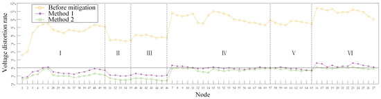
Figure 22.
Total harmonic voltage distortion rate of each node before and after mitigation in Scenario 2.
The effect of increasing the weighting factor on the harmonic distributed mitigation system is further discussed. The THDv at each node after mitigation using = 0.8 is shown in Figure 23. Compared with the mitigation effect at = 0.5, the THDv of each node is lower with = 0.8, and especially method 2 can effectively reduce the THDv. This indicates that appropriately increasing the value of can improve the positivity of the mitigation devices and the effect of harmonic mitigation of the whole system. Therefore, the weighting coefficients can be adjusted according to different operational requirements to achieve the harmonic mitigation of the system.
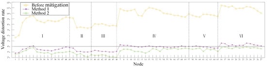
Figure 23.
The total harmonic voltage distortion rate of each node before and after mitigation in Scenario 2 when = 0.8.
Through a comprehensive analysis of the IEEE 69-bus simulation experiment, the distributed mitigation method of six mitigation devices shows good applicability and effectiveness in larger-scale grid systems. The mitigation strategy of partition adjustment and regional mutual assistance significantly improves the harmonic mitigation effect, and the compensation capacity of each mitigation device is fully utilized to keep the THDv of the system at a low level.
5.6. Hardware Experiment
In order to enhance the reliability and scientific rigor of this study’s conclusions, this study also implemented hardware experiments and adopted the OPAL-RT system to examine the operational performance of the VDAPF. Specifically, the OPAL-RT system boasts high-precision and real-time simulation capabilities that enable detailed monitoring and analysis of the harmonics in the power grid, as shown in Figure 24.

Figure 24.
OPAL-RT system.
Firstly, the FFT spectrum of the VDAPF injection current was analyzed using the OPAL-RT system, as shown in Figure 25. The spectrogram clearly shows the major harmonic frequency components, where distinct high-frequency noise indicates the presence of harmonic pollution problems in the grid. By analyzing these high-frequency components, the specific harmonic frequencies that require mitigation can be precisely identified. This allows the VDAPF to tailor its intervention, generating equal-amplitude reverse harmonic currents for effective harmonic mitigation.
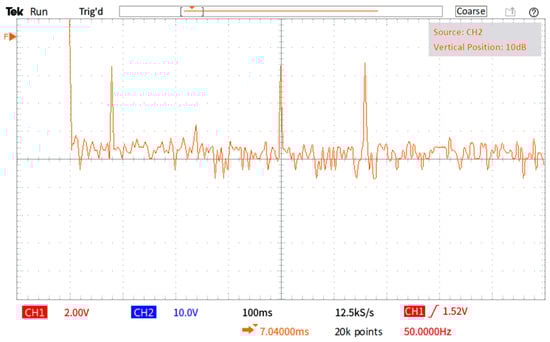
Figure 25.
VDAPF injection current FFT spectrum analysis.
Secondly, the compensation current injected by the VDAPF was studied in detail, as shown in Figure 26. The waveforms and amplitudes of the compensation currents were analyzed to evaluate the compensation capability of the VDAPF under different load conditions.
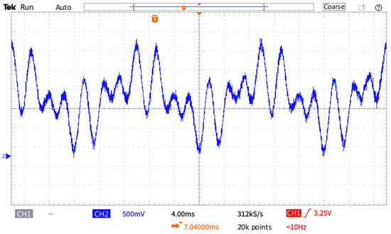
Figure 26.
VDAPF injection compensation current.
Finally, the voltage waveforms after VDAPF mitigation were observed and recorded, as shown in Figure 27. By comparing the voltage waveforms before and after mitigation, the effectiveness of VDAPF in improving power quality was evaluated. The results show that the voltage waveforms after VDAPF mitigation are smoother and close to the ideal sinusoidal waveforms. Additionally, the significant reduction in harmonic content confirms the VDAPF is effective in reducing harmonics in the power grid.
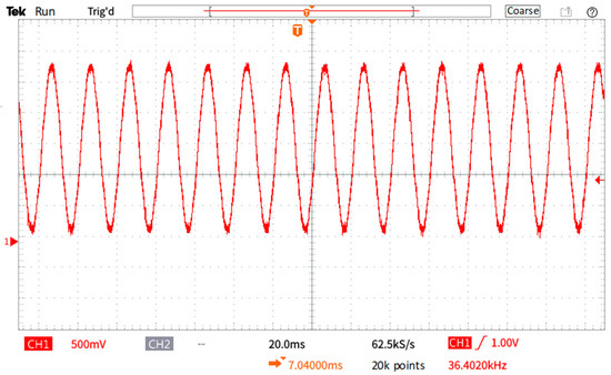
Figure 27.
Voltage waveform after VDAPF processing.
In summary, this study comprehensively and meticulously analyzes the injected currents and treated voltage waveforms of the VDAPF by means of the OPAL-RT system. Combined with simulation and experimental data, the important role of VDAPFs in harmonic mitigation and power quality improvement is shown. This study further validates the effectiveness and adaptability of the strategy of harmonic mitigation in this paper.
6. Conclusions
(1) The community thinking of the blockchain is applied to the distributed harmonic mitigation system to realize the decentralization of centralized computing power to distributed computing power. The value of residual compensation capacity is fully utilized through the active mitigation mode of the mitigation device. Through the mitigation model of regional mutual assistance, the problem of insufficient VDAPF mitigation capacity in some mitigation areas in the fully distributed mitigation system is solved.
(2) Through the comprehensive voltage sensitivity analysis of each harmonic setting weight, the difference in each harmonic is fully considered, and a more accurate partition result is obtained. The partition process ensures that each mitigation node is divided into the region where the VDAPF region with the strongest mitigation ability is located by determining the mitigation node first and then the mitigation node. Harmonic pollution is not very serious; only reliance on partition mitigation can achieve a qualified mitigation effect.
(3) Each mitigation device in each region is given the role of a miner in the blockchain, and a harmonic mitigation strategy based on dynamic integral excitation of self-learning algorithms is established. By defining the calculation method of the mitigation integral, based on not increasing the mitigation device, each mitigation device obtains the integral active output. The THDv of each node meets the requirements through partition adjustment and regional cooperation, which solves the problem that the harmonic voltage distortion rate of the mitigation node exceeds the limit caused by the insufficient mitigation capacity of individual regions when encountering large harmonic pollution.
The simulation results verify the model’s effectiveness and adaptability in maintaining the frequency stability of the grid and demonstrate a significant improvement in the harmonic dynamic response capability. The model successfully copes with harmonic pollution in different scenarios, especially in the heavy pollution scenario, and adjusts the action strategy of the harmonic mitigation device by optimizing the mutual assistance mechanism among the regions, which ensures a significant reduction in the harmonic voltage distortion rate and meets the requirements of the stable operation of the grid.
The method proposed in this study faces certain limitations in practical applications because of the integration of blockchain technology, which increases the computational overhead in areas such as smart contract execution, network communication, and data storage. An important future research direction is to explore how to solve these problems in order to increase the practical application value of the proposed method and reduce the energy consumption and computational overhead of the system devices.
Author Contributions
Conceptualization, L.W. and J.F. methodology, J.F. and W.Z.; software, C.S.; validation, W.Z. and C.S.; formal analysis, L.W., J.F. and W.Z.; investigation, W.K.; resources, P.L. and J.F.; data curation, L.W.; writing—original draft, J.F. and W.Z.; writing—review and editing, W.K. and J.F.; visualization, P.L.; supervision, C.S.; project administration, L.W.; funding acquisition, W.Z. All authors have read and agreed to the published version of the manuscript.
Funding
This work was supported by the Science and Technology Project of State Grid Hebei Electric Power Co., Ltd., in 2023 (SGHEDK00JSJS2310221) and the National Nature Science Foundation of China (NSFC) under project number 51877186.
Data Availability Statement
The original contributions presented in the study are included in the article, further inquiries can be directed to the corresponding author.
Acknowledgments
We thank the reviewers for their useful comments and suggestions.
Conflicts of Interest
Authors Lei Wang, Wen Zhou and Can Su were employed by the company State Grid Hebei Electric Power Research Institute. The remaining authors declare that the research was conducted in the absence of any commercial or financial relationships that could be construed as a potential conflict of interest. The authors declare that this study received funding from Science and Technology Project of State Grid Hebei Electric Power Co., Ltd. The funder was not involved in the study design, collection, analysis, interpretation of data, the writing of this article or the decision to submit it for publication.
Appendix A
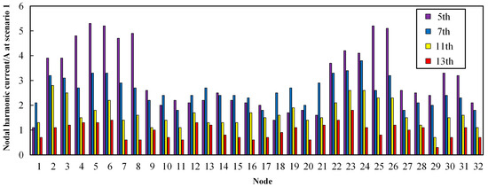
Figure A1.
Harmonic current injection under Scenario 1.
Figure A1.
Harmonic current injection under Scenario 1.

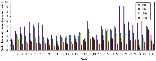
Figure A2.
Harmonic current injection under scenario 2.
Figure A2.
Harmonic current injection under scenario 2.

Appendix B
| SN | Symbol/ Formula | Meaning/Definition | First Appearance |
|---|---|---|---|
| 1 | DG | distributed generator | Section 1 |
| 2 | is the set of VDAPF vertices, is the set of edges, and is the adjacency matrix of graph | Section 2.3 | |
| 3 | number of VDAPF units | Section 2.3 | |
| 4 | the degree matrix of the graph | Section 2.3 | |
| 5 | the degree of vertex | Section 2.3 | |
| 6 | elements in the set of edges connected by vertices | Section 2.3 | |
| 7 | an element of the adjacency matrix | Section 2.3 | |
| 8 | high-pass filter | Section 3.1 | |
| 9 | integrated sensitivity matrix | Section 3.2.2 | |
| 10 | the harmonic voltage of controlled node | Section 3.2.1 | |
| 11 | value of harmonic conductance of VDAPF at control node | Section 3.2.1 | |
| 12 | column vector of harmonic voltages | Section 3.2.1 | |
| 13 | column vector of harmonic currents | Section 3.2.1 | |
| 14 | harmonic conductivity matrix | Section 3.2.1 | |
| 15 | equivalent conductance of mitigation node | Section 3.2.1 | |
| 16 | injection of harmonic currents at mitigation node | Section 3.2.1 | |
| 17 | the portion of the self-conductance of node after removing | Section 3.2.1 | |
| 18 | network parameter constants | Section 3.2.1 | |
| 19 | harmonic weighting factor | Section 3.2.2 | |
| 20 | integrated sensitivity | Section 3.2.2 | |
| 21 | the coupling between nodes corresponding to the harmonic | Section 3.3 | |
| 22 | integrated coupling of harmonic voltages at nodes | Section 3.3 | |
| 23 | electrical distance between nodes | Section 3.3 | |
| 24 | fxpression Factor | Section 4.1.1 | |
| 25 | subtotal global effect factor for assisted mitigation | Section 4.1.1 | |
| 26 | sum of weighted harmonic voltage distortion rates at all nodes of the system | Section 4.1.1 | |
| 27 | the value of the distortion rate corresponding to the minimum standard for voltage compliance | Section 4.1.1 | |
| 28 | weights set according to the differentiated needs of different nodes for harmonic levels | Section 4.1.1 | |
| 29 | the -sensitivity factor of the sensitivity factor | Section 4.1.1 | |
| 30 | total voltage distortion rate of controlled node | Section 4.1.1 | |
| 31 | RMS value of the fundamental voltage at node | Section 4.1.1 | |
| 32 | individual performance factor for the assisted mitigation device | Section 4.1.1 | |
| 33 | degree of motivation of a mitigation device to participate in assisting mitigation | Section 4.1.1 | |
| 34 | actual compensated capacity before/after assisted mitigation for VDAPFs, rated capacity | Section 4.1.1 | |
| 35 | the harmonic voltage at node | Section 4.1.1 | |
| 36 | refers to the performance factor of the VDAPF under the assisted mitigation | Section 4.1.1 | |
| 37 | weighting factors | Section 4.1.1 | |
| 38 | the positivity factor of a piece of a mitigation device | Section 4.1.1 | |
| 39 | value of harmonic conductance after accessing VDAPF regulation at node | Section 4.1.2 | |
| 40 | modulation of the harmonic conductance | Section 4.1.2 | |
| 41 | actual value of h-harmonic voltage adjusted at node where the VDAPF is located | Section 4.1.2 | |
| 42 | assisted compensation capacity of the mitigation device | Section 4.2 | |
| 43 | mitigation device optimal compensation capacity obtained through optimization or training | Section 4.2 | |
| 44 | device number of adjustment steps required to achieve optimum compensation capacity | Section 4.2 | |
| 45 | maximum assisted compensation capacity | Section 4.2 | |
| 46 | device maximum integral value when using | Section 4.2 | |
| 47 | adjusted steps to assist with force generation | Section 4.2 | |
| 48 | individual performance factor for the governance device | Section 4.3 | |
| 49 | indicator scores for determining weighting factors | Section 5.1 | |
| 50 | Total Harmonic Distortion of Voltage | Section 5.4 | |
| 51 | Fast Fourier Transform | Section 5.6 |
References
- Gong, C.; Cheng, Z.; Sou, W.K.; Lam, C.S.; Chow, M.Y. Collaborative Distributed Optimal Control of Pure and Hybrid Active Power Filters in Active Distribution Network. IEEE Trans. Power Deliv. 2023, 38, 2326–2337. [Google Scholar] [CrossRef]
- Liu, Q.; Li, Y.; Luo, L.; Peng, Y.; Cao, Y. Power Quality Mitigation of PV Power Plant with Transformer Integrated Filtering Method. IEEE Trans. Power Deliv. 2019, 34, 941–949. [Google Scholar] [CrossRef]
- Jarwar, A.R.; Soomro, A.M.; Memon, Z.A.; Odhano, S.A.; Uqaili, M.A.; Larik, A.S. High Dynamic Performance Power Quality Conditioner for AC Microgrids. IET Power Electron. 2019, 12, 550–556. [Google Scholar] [CrossRef]
- Ruiz-Rodriguez, F.J.; Hernandez, J.C.; Jurado, F. Iterative Harmonic Load Flow by Using the Point-Estimate Method and Complex Affine Arithmetic for Radial Distribution Systems with Photovoltaic Uncertainties. Int. J. Electr. Power Energy Syst. 2020, 118, 105765. [Google Scholar] [CrossRef]
- Hernandez, J.C.; Ruiz-Rodriguez, F.J.; Jurado, F.; Sanchez-Sutil, F. Tracing Harmonic Distortion and Voltage Unbalance in Secondary Radial Distribution Networks with Photovoltaic Uncertainties by an Iterative Multiphase Harmonic Load Flow. Electr. Power Syst. Res. 2020, 185, 106342. [Google Scholar] [CrossRef]
- Abu-Jalala, A.-H.M.; Cox, T.; Gerada, C.; Rashed, M.; Hamiti, T.; Brown, N. Power Quality Improvement of Synchronous Generators Using an Active Power Filter. IEEE Trans. Ind. Appl. 2018, 54, 4080–4090. [Google Scholar] [CrossRef]
- Akagi, H.; Fujita, H.; Wada, K. A Shunt Active Filter Based on Voltage Detection for Harmonic Termination of a Radial Power Distribution Line. IEEE Trans. Ind. Appl. 1999, 35, 638–645. [Google Scholar] [CrossRef]
- Akagi, H. Control Strategy and Site Selection of a Shunt Active Filter for Damping of Harmonic Propagation in Power Distribution Systems. IEEE Trans. Power Deliv. 1997, 12, 354–363. [Google Scholar] [CrossRef]
- Wada, K.; Fujita, H.; Akagi, H. Considerations of a Shunt Active Filter Based on Voltage Detection for Installation on a Long Distribution Feeder. IEEE Trans. Ind. Appl. 2002, 38, 1123–1130. [Google Scholar] [CrossRef]
- Xiaofeng, S.; Jian, Z.; Fang, Z.; Li, X. Site Selection Strategy of Discrete Frequency Resistive Active Power Filter. Proc. CSEE 2011, 31, 65–70. [Google Scholar]
- Lee, T.-L.; Cheng, P.-T.; Akagi, H.; Fujita, H. A Dynamic Tuning Method for Distributed Active Filter Systems. IEEE Trans. Ind. Appl. 2008, 44, 612–623. [Google Scholar] [CrossRef]
- Vahedi, H.; Shojaei, A.A.; Dessaint, L.A.; Al-Haddad, K. Reduced DC-Link Voltage Active Power Filter Using Modified PUC5 Converter. IEEE Trans. Power Electron. 2018, 33, 943–947. [Google Scholar] [CrossRef]
- Panigrahi, R.; Subudhi, B. Performance Enhancement of Shunt Active Power Filter Using a Kalman Filter-Based H∞ control Strategy. IEEE Trans. Power Electron. 2017, 32, 2622–2630. [Google Scholar] [CrossRef]
- França, B.W.; Aredes, M.; Da Silva, L.F.; Gontijo, G.F.; Tricarico, T.C.; Posada, J. An Enhanced Shunt Active Filter Based on Synchronverter Concept. IEEE J. Emerg. Sel. Top. Power Electron. 2022, 10, 494–505. [Google Scholar] [CrossRef]
- Shi, L.; Jia, Q.; Lin, L.; Wang, N.; Tian, G. Distributed Global Optimal Harmonic Mitigation Strategy for Power Electronics High Penetrated Distribution Networks. Proc. CSEE 2020, 40, 2914–2924. [Google Scholar]
- Jintakosonwit, P.; Akagi, H.; Fujita, H.; Ogasawara, S. Implementation and Performance of Automatic Gain Adjustment in a Shunt-Active Filter for Harmonic Damping throughout a Power Distribution System. IEEE Trans. Power Electron. 2002, 17, 438–447. [Google Scholar] [CrossRef]
- Lakum, A.; Mahajan, V. Optimal Placement and Sizing of Multiple Active Power Filters in Radial Distribution System Using Grey Wolf Optimizer in Presence of Nonlinear Distributed Generation. Electr. Power Syst. Res. 2019, 173, 281–290. [Google Scholar] [CrossRef]
- Lakum, A.; Mahajan, V. A Novel Approach for Optimal Placement and Sizing of Active Power Filters in Radial Distribution System with Nonlinear Distributed Generation Using Adaptive Grey Wolf Optimizer. Eng. Sci. Technol. Int. J. 2021, 24, 911–924. [Google Scholar] [CrossRef]
- Carpinelli, G.; Proto, D.; Russo, A. Optimal Planning of Active Power Filters in a Distribution System Using Trade-off/Risk Method. IEEE Trans. Power Deliv. 2017, 32, 841–851. [Google Scholar] [CrossRef]
- Moradifar, A.; Akbari Foroud, A. A Hybrid Fuzzy DIAICA Approach for Cost-Effective Placement and Sizing of APFs. IETE Tech. Rev. 2017, 34, 579–589. [Google Scholar] [CrossRef]
- Li, G.; Guan, X.; Yang, H.; Zhao, L.; Xin, R.; Chen, L. Peer-to-Peer Energy Trading Strategy of Microgrid Based on Smart Contract. CAAI Trans. Intell. Syst. 2023, 18, 813–822. [Google Scholar]
- Zhang, L.; Chen, S.; Yan, Z.; Shen, Z. Distributed Multi-Area Optimal Power Flow Algorithm Based on Blockchain Consensus Mechanism. Proc. CSEE 2020, 40, 6433–6441. [Google Scholar]
- Wang, J.; Zhou, N.; Wang, Q.; Wang, P. Electricity Direct Transaction Mode and Strategy in Microgrid Based on Blockchain and Continuous Double Auction Mechanism. Proc. CSEE 2018, 38, 5072–5084. [Google Scholar]
- Ping, J.; Chen, S.; Zhang, N.; Yan, Z.; Yao, L. Decentralized Transactive Mechanism in Distribution Network Based on Smart Contract. Proc. CSEE 2017, 37, 3682–3690. [Google Scholar]
- Zhou, K.; Chong, J.; Lu, X.; Yang, S. Credit-Based Peer-to-Peer Electricity Trading in Energy Blockchain Environment. IEEE Trans. Smart Grid 2022, 13, 678–687. [Google Scholar] [CrossRef]
- Chen, S.; Zhang, L.; Yan, Z.; Shen, Z. A Distributed and Robust Security-Constrained Economic Dispatch Algorithm Based on Blockchain. IEEE Trans. Power Syst. 2022, 37, 691–700. [Google Scholar] [CrossRef]
- Yang, N.C.; Adinda, E.W. Matpower-Based Harmonic Power Flow Analysis for Power Systems with Passive Power Filters. IEEE Access 2021, 9, 167322–167331. [Google Scholar] [CrossRef]
- Santos, G.G.; Oliveira, T.L.; Oliveira, J.C.; Vieira, J.C.M. A Hybrid Method for Harmonic State Estimation in Partially Observable Systems. Int. Trans. Electr. Energy Syst. 2021, 31, e12763. [Google Scholar] [CrossRef]
- Safargholi, F.; Malekian, K. Relevant Factors for Evaluation of the Harmonic Responsibility of Utility and Customer. IEEE Trans. Power Deliv. 2021, 36, 124–134. [Google Scholar] [CrossRef]
- Yun, Z.; Cui, X.; Ma, K. Online Thevenin Equivalent Parameter Identification Method of Large Power Grids Using LU Factorization. IEEE Trans. Power Syst. 2019, 34, 4464–4475. [Google Scholar] [CrossRef]
- Chen, J.; Yue, D.; Dou, C.; Li, Y.; Hancke, G.P.; Weng, S.; Guerrero, J.M.; DIng, X. Distributed Control of Multi-Functional Grid-Tied Inverters for Power Quality Improvement. IEEE Trans. Circuits Syst. I Regul. Pap. 2021, 68, 918–928. [Google Scholar] [CrossRef]


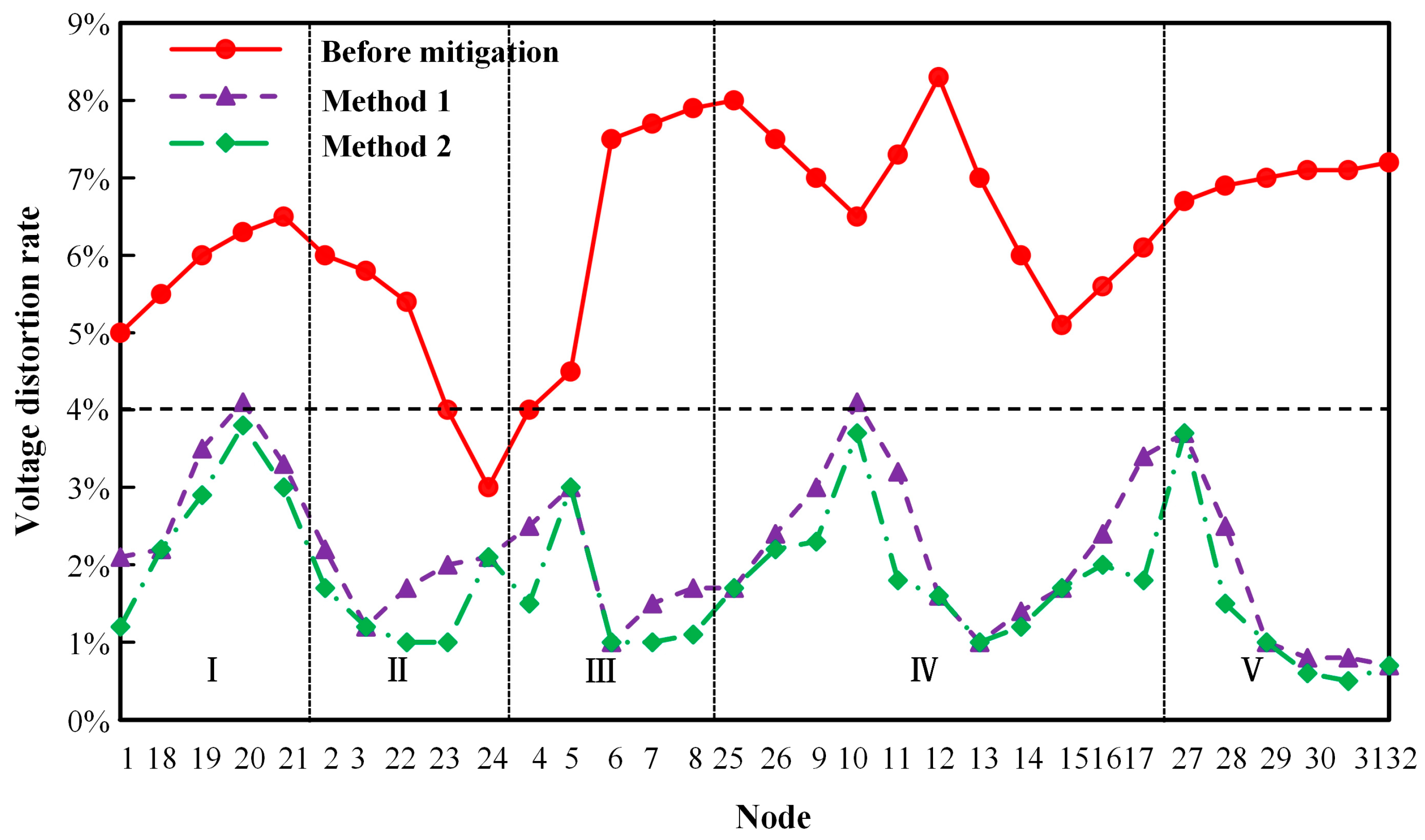


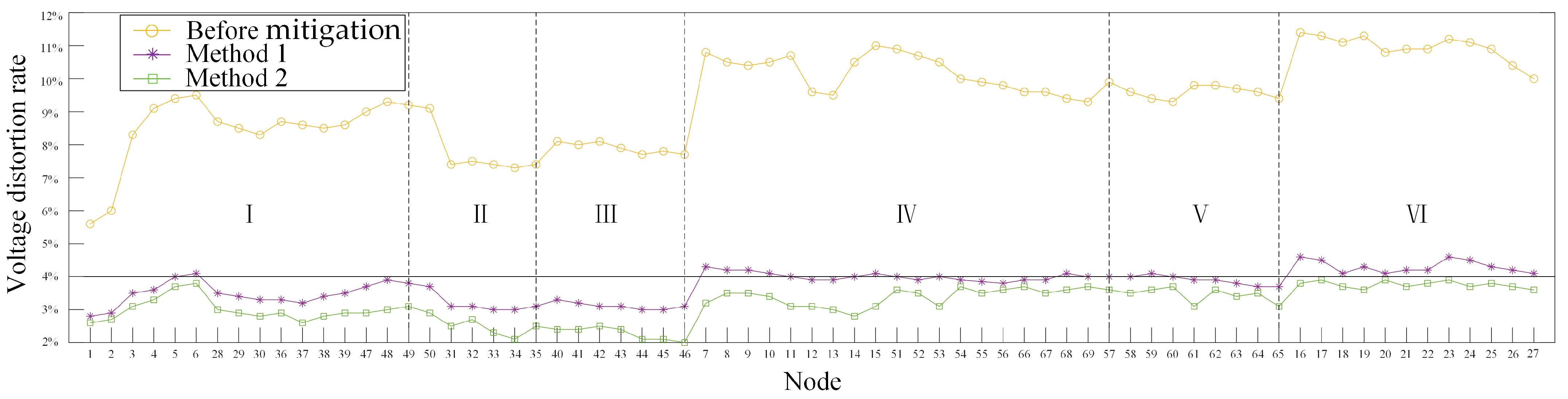
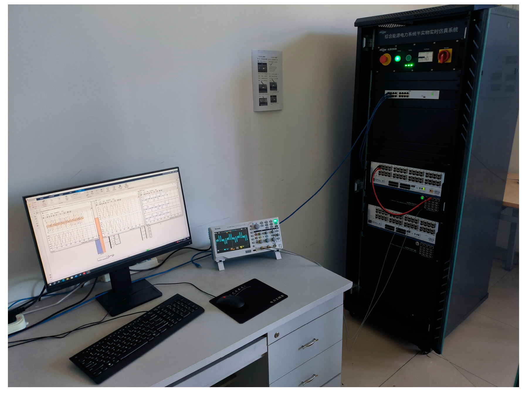


Disclaimer/Publisher’s Note: The statements, opinions and data contained in all publications are solely those of the individual author(s) and contributor(s) and not of MDPI and/or the editor(s). MDPI and/or the editor(s) disclaim responsibility for any injury to people or property resulting from any ideas, methods, instructions or products referred to in the content. |
© 2024 by the authors. Licensee MDPI, Basel, Switzerland. This article is an open access article distributed under the terms and conditions of the Creative Commons Attribution (CC BY) license (https://creativecommons.org/licenses/by/4.0/).