Control and Stability of Grid-Forming Inverters: A Comprehensive Review

Abstract

The large integration of inverter-based resources will significantly alter grid dynamics, leading to pronounced stability challenges due to fundamental disparities between inverter-based and traditional energy systems. While grid-following inverters (GFLIs) dominate current inverter configurations, their increased penetration into the grid can result in major stability issues. In contrast, grid-forming inverters (GFMIs) excel over GFLIs by offering features like standalone operation, frequency support, and adaptability in weak grid scenarios. GFMIs, unlike GFLIs, control the AC voltage and frequency at the common coupling point, impacting the inverter dynamic response to grid disturbances and overall stability. Despite the existing literature highlighting differences between GFLIs and GFMIs and their control strategies, a comprehensive review of GFMIs’ stability and the effects of their control schemes on grid stability is lacking. This paper provides an in-depth evaluation of GFMIs’ stability, considering various control schemes and their dynamics. It also explores different types of power system stability, introduces new stability concepts that correspond to power grids with integrated inverters, i.e., resonance and converter-driven stability, and reviews small-signal and transient stability analyses, which are the main two types of GFMI stability studied in the literature. The paper further assesses existing studies on GFMI stability, pinpointing research gaps for future investigations.

1. Introduction

The considerable integration of renewable energy sources (RESs), modern loads such as electric vehicles, and transmission of power over high-voltage direct current (HVDC) lines has resulted in the connection of a large number of converters to the power grid [1,2,3,4,5,6]. The power grid is anticipated to transform into a fully inverter-based system. This transformation will result in major changes in the structure and operational dynamics of electrical power systems [1,2,3,4,5,6] leading to significant stability issues due to inherent differences between dynamics of inverters and synchronous generators (SGs) [7,8].

There are two types of inverters used in the power grid: grid-following inverters (GFLIs) and grid-forming inverters (GFMIs). The control system of GFLIs controls their output current while following the voltage magnitude and frequency at the point of connection to the alternating current (AC) grid using a phase-locked loop (PLL) [1,9]. Most of the inverters used in the power grid are GFLIs [1,10]. An increased penetration of GFLIs into the grid can result in major stability issues [10]. The oscillatory stability events in GFLIs of HVDC systems are reviewed in [8]. Voltage and current oscillations at the testing stage of Nanhui HVDC system in Shanghai, China, in 2011 are reported in [8,11]. Output current oscillations in the Xiamen HVDC system in Fujian, China, in 2015 are reported in [8,12]. High-frequency current oscillations in the Borwin1 HVDC system in North Sea, Germany, in 2013 are reported in [8,13]. Current oscillations in the Luxi HVDC system in Yunnan, China, in 2017 are another example of oscillatory stability issues of GFLIs [8,14].

Voltage and current oscillations can happen when a GFLI is connected to a weak grid due to errors in the estimated frequency by the PLL [15,16]. Changes in the loading condition of a GFLI may also result in instability as its output power does not change. This constant output power leads to voltage oscillations in the system, which cause errors in the PLL. These errors lead to output power oscillations in the GFLI. If another generation unit damps these oscillations, the GFLI continues its operation at its output power set-point. Otherwise, the oscillations will be sustained [10]. Reference [17] shows that switching the control scheme of the inverter from GFLI to GFMI in critical stability conditions helps the system remain stable. In contrast to GFLIs, the control of GFMIs is based on controlling the AC voltage magnitude and frequency at the point of common coupling (PCC). This characteristic of GFMIs allows them to operate in the stand-alone mode [1]. Moreover, GFMIs are stable when connected to weak grids, as their control scheme does not require a PLL for grid synchronization [9]. Operation in the stand-alone mode [18], frequency support [18], and ability to operate under weak grid conditions [9] are among the main advantages of GFMIs over GFLIs. The study of [19] shows that compared to GFLIs, grid-connected GFMIs can supply larger loads while maintaining small-signal stability.

There are several examples of grid-forming pilot projects around the world [20]. The Zurich battery energy storage system (BESS) project in Dietikon, Switzerland, started in 2012 and the BESS has been operative since 2014. The main features of this project are primary frequency control, peak shaving, and islanded operation. This BESS has a rated power of 1 MW and a capacity of 580 kWh and is designed for both low-voltage and medium-voltage connections [20,21]. The AusNet Grid Energy Storage System (GESS) project in Thomastown, Australia, started in 2012. The GESS consists of a 1 MW/1 MWh lithium-ion battery system connected to the grid by a 1.37 MVA GFMI and a 1 MVA backup diesel generator. The GESS project provides peak shaving, voltage support, power factor correction, and islanded operation [20,22].

The Mackinac HVDC system project is another example of GFMI projects which started in 2012 and was operated in 2014 to control the power flow between Michigan’s upper and lower peninsula. The Mackinac HVDC system with GFMIs can operate when connected to a weak grid and provides voltage oscillation mitigation [20,23]. This HVDC system transfers a bidirectional power of 200 MW and 100 MVAR using two converters that are connected directly to each other [24]. The south converter is controlled using vector current control scheme and the north GFMI is controlled using the frequency-droop control scheme and direct voltage magnitude control [24]. The Dersalloch wind farm in Dersalloch, Scotland, was operated in the grid-forming mode from May to June 2019 to provide inertia to the system. The 69 MW Dersalloch wind farm has twenty three 3 MW direct drive full converter wind power generators [20]. The Hornsdale Power Reserve BESS project started in Jamestown, south Australia, in 2017. The power capacity of the plant is 150 MW and it has an energy capacity of 194 MWh. It is connected to the grid at 275 kV voltage level. This BESS provides fast frequency response and inertia to the system [20,25,26].

The ES CRI-SA BESS located near the Dalrymple substation in south Australia, was commissioned in 2017. The ES CRI-SA BESS has a power capacity of 30 MW and an energy capacity of 8 MWh. The ES CRI-SA BESS is connected to the 33 kV grid and provides ancillary frequency services and fast frequency response, and reduces failures in energy supply in case of islanding [20,27]. The St. Eustatius II project in St. Eustatius, Caribbean, started in 2017. A diesel generation of 4 MVA, solar power of 4.15 MW, and a BESS of 5.9 MWh capacity form the generation and storage mix of this project. Three GFMIs, two with a capacity of 2.2 MW and one with a capacity of 1 MW, are used in St. Eustatius II project to make 100% use of solar power [20,28]. A hybrid power plant started in La Plana, Spain, in 2015. The plant consists of a wind power generation of 850 kW, solar power generation of 245 kW, diesel generation of 222 kW, and a BESS of 545 kWh capacity. The GFMIs used in this plant provide ancillary services such as peak shaving, frequency regulation, and frequency reserve [20].

Reference [1] provides a review of several GFMI control schemes, as well as challenges related to the integration of GFMIs in the grid. Reference [1] provides a brief overview of stability studies, real-world implementations, and grid applications of GFMIs. Reference [29] offers a detailed exploration of the differences between GFMIs and GFLIs, the topologies of GFMIs, their hierarchical control strategy, the structures of inner and outer control loops, control schemes for GFMIs, and the diverse applications of GFMIs within power grids. Reference [30] compares GFLIs and GFMIs and reviews different grid-forming control schemes, their modeling, and design considerations. The control scheme of GFMIs affects their dynamic response to disturbances in the grid and, thus, their stability [31]. Although the existing reviews of [1,29,30] elaborate on the differences between GFLIs and GFMIs, their control schemes, and new concepts related to GFMIs, none of them provide a comprehensive review of GFMIs’ stability issues and how their control schemes affect their stability. This paper presents an extensive review and evaluation of the stability aspects of GFMIs, delving into the dynamics of various GFMI control schemes and their impact on system stability. It also discusses various methods found in the existing literature for analyzing the stability of GFMIs, along with presenting multiple strategies proposed to enhance the stability performance of these systems.

In this paper, first, various control schemes for GFMIs such as frequency-droop control [32], angle-droop control [33], power synchronization control (PSC) [34], synchronverter [35], virtual synchronous machine (VSM) [36,37], matching control [38,39,40], virtual oscillator control (VOC) [41], and dispatchable VOC (dVOC) [42] are reviewed and their block diagrams, dynamics, and features are presented. Although other GFMI control schemes such as configurable natural droop [1,43], generalized droop control [1,44], unified voltage oscillator control [1,45], $H_{\infty }\setminus H_2$-based robust fixed-structure control [1,46,47], and frequency shaping-based control [1,48] are proposed in the literature, only control schemes that are considered in stability analyses of GFMIs are reviewed. Second, various types of stability in power systems such as voltage, rotor angle, and frequency, as well as two new stability types that correspond to power grids with integrated inverters, i.e., resonance and converter-driven, are discussed. Third, small-signal stability and transient stability, which are the main two types of GFMI stability studied in the literature, are reviewed, and different methods of stability analysis, which are used in the literature, are presented. Finally, the existing studies of GFMI stability in the literature are reviewed, and the gaps to be addressed for future research are identified.

The rest of the paper is organized as follows: in Section 2, GFLIs, GFMIs, and their corresponding control systems are reviewed. In Section 3, inner control loops and main control schemes for outer control loops of GFMIs are presented. In Section 4, power system stability definitions, various types of analysis tools, as well as existing literature on stability of GFMIs are discussed. Discussions and conclusions are presented in Section 6 and Section 7.

2. Grid-Following and Grid-Forming Inverters

In this section, the operating principle of GFLIs and GFMIs as well as their control system are introduced.

2.1. Grid-Following Inverters

Most of inverters in the power grid are GFLIs [1]. With GFLIs, the power transferred to the grid at PCC is controlled according to power references $P_{ref}$ and $Q_{ref}$. Assuming the voltage at the PCC is constant, this power transfer would be equivalent to injecting a certain amount of current into the power grid; thus, GFLIs can be modeled as current sources, as shown in Figure 1 [9].

In Figure 1, $I_{ref}$, ${\theta }_{ref}$, $Y_{eq}$, and $L_g$ are the reference output current, the estimated phase angle of the PCC voltage, the output admittance of the GFLI, and the inductance of the transmission line connecting the GFLI to the grid, respectively. The control of GFLIs depends on the measured voltage and the estimated frequency of the grid. In GFLIs, the output voltage and frequency are not directly controlled. A simple schematic of a typical GFLI and its control is shown in Figure 2.

In Figure 2, $i_t$, $i_g$, $V_t$, $V_c$, and $V_g$ are the output current of the inverter, grid-side current of the inverter, output voltage of the inverter, PCC voltage, and grid voltage, respectively. $I_{tdq}$, $I_{gdq}$, and $V_{cdq}$ are the direct-quadrature-zero (dq0) reference frame representations of the inverter output current, grid-side current, and PCC voltage, respectively. $P_{ref}$, $Q_{ref}$, ${\theta }_{ref}$, $V_{tref}$, and m are the output active power reference, output reactive power reference, estimated phase angle of the PCC voltage, voltage reference at the inverter terminal, and the switching signal, respectively. P, Q, $L_c$, $C_f$, and $L_g$ are the output active power, output reactive power, output filter inductance, output filter capacitance, and transmission line inductance, respectively. $R_{dc}$, $C_{dc}$, $I_{dcref}$, $i_{dc}$, and $V_{dc}$ are the direct current (DC)-side capacitance, resistance, DC-side reference current, input current of the inverter, and DC link voltage, respectively.

The control of GFLIs typically takes place in the dq0 reference frame [49]. The PLL and outer and inner control loops are the main control loops of a GFLI [1]. The reference angular speed ${\omega }_{ref}$ and ${\theta }_{ref}$ are estimated using a PLL [1]. In most systems, a synchronous reference frame PLL (SRF-PLL) is used for controlling GFLIs because of its well-known structure and robust performance [50]. As shown in Figure 3, an SRF-PLL typically consists of a proportional-integral (PI) controller and an integrator [50]. It estimates ${\omega }_{ref}$ by setting the quadrature component of its input voltage, $V_{cq}$, to zero using the PI controller [50]. Then, ${\theta }_{ref}$ is derived by integrating ${\omega }_{ref}$. The output of the PLL, ${\theta }_{ref}$, is used as the reference angle in any dq-to-abc or abc-to-dq transformation in the system [51].

Using PI controllers, $I_{tdref}$ and $I_{tqref}$ are generated in the outer control loop, as shown in Figure 3 [49]. The dynamics of $I_{td}$ and $I_{tq}$ are shown in (1) and (2).

$$L_c\frac{d{I}_{td}}{dt}=L_c{\omega }_{ref}{I}_{tq}+V_{td}-V_{cd},$$

(1)

$$L_c\frac{d{I}_{tq}}{dt}=-L_c{\omega }_{ref}{I}_{td}+V_{tq}-V_{cq}.$$

(2)

Using the feed-forward signals in the inner control loop, shown in Figure 3, the dynamics of $I_{td}$ and $I_{tq}$ are simplified as shown in Figure 4 and (3) and (4), where $u_{id}$ and $u_{iq}$ are the controller output signals. Then, as illustrated in Figure 3, $V_{tdref}$ and $V_{tqref}$ are generated using PI controllers in the inner control loop.

$$L_c\frac{d{I}_{td}}{dt}=u_{id},$$

(3)

$$L_c\frac{d{I}_{tq}}{dt}=u_{iq}.$$

(4)

Since GFLIs do not form the voltage magnitude and frequency of the PCC, these inverters cannot operate in the stand-alone mode [1,9]. Moreover, PLLs estimate the frequency of the PCC voltage [1,7]. When GFLIs are connected to weak grids, possible fast electromagnetic transients in their output voltages may result in the PLL estimating the frequency of these transients and causing loss of synchronization between GFLIs and the grid [7]. PLLs also have a delay when estimating the frequency, which can affect the performance of the control loops of GFLIs. GFMIs can operate in the stand-alone mode and do not require a PLL for synchronization to the grid. Therefore, they can replace GFLIs to avoid the aforementioned issues [1].

2.2. Grid-Forming Inverters

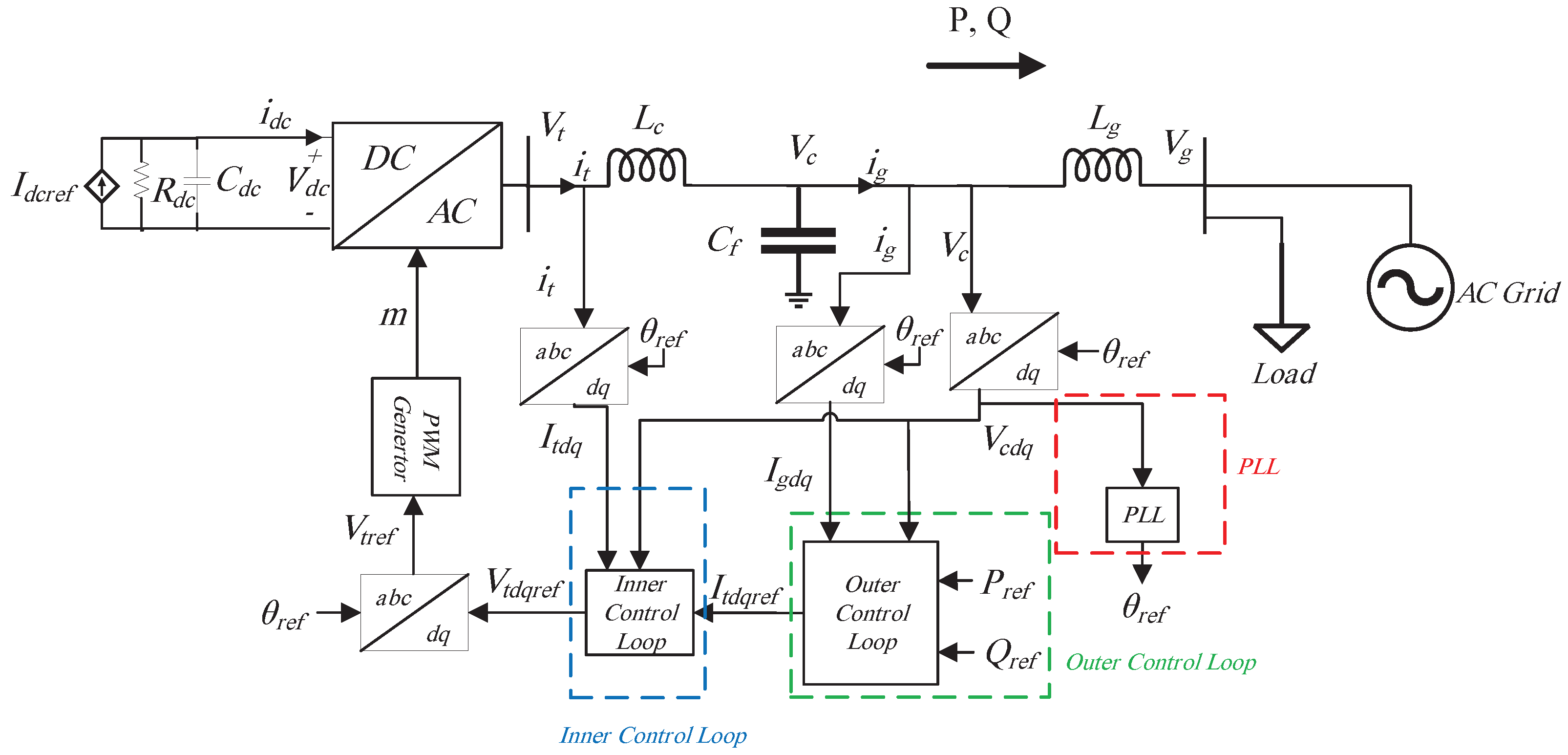
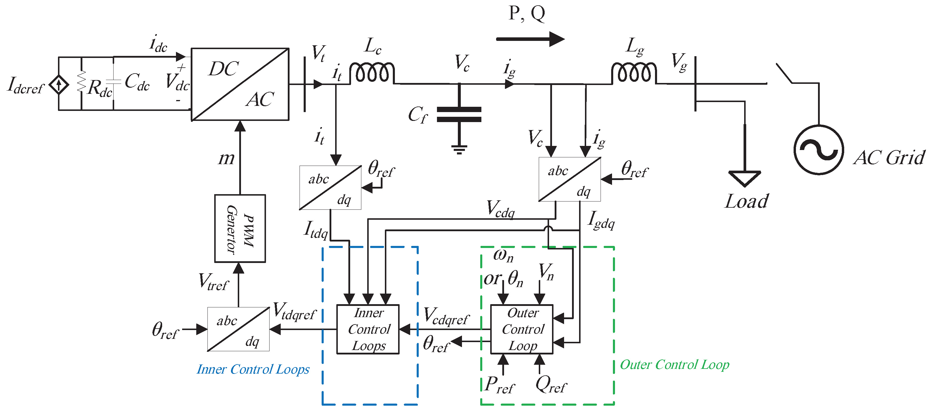
Unlike GFLIs, GFMIs control the grid voltage and frequency. Thus, GFMIs can be modeled as controlled voltage sources [52], as shown in Figure 5.

In Figure 5, $V_{ref}$, ${\theta }_{ref}$, $Z_{eq}$, and $L_g$ are the reference terminal voltage, reference phase angle for the PCC voltage, output impedance of the GFMI, and the inductance of the transmission line connecting the GFMI to the grid, respectively. GFMIs can be controlled to inject the reference active and reactive power into the grid. To improve the output voltage and current quality of the inverter, different types of harmonic filters, such as L-filters, LC-filters, and LCL-filters, are used at the inverter terminal [29,53]. Although simple in design, L-filters do not provide proper harmonic damping, and may result in significant voltage drop across the inductor. In comparison to L-filters, LC- and LCL-filters can provide better harmonic damping and a lower voltage drop across the filters [29,53]. The schematic of a typical GFMI is shown in Figure 6.

In Figure 6, $i_t$, $i_g$, $V_t$, $V_c$, and $V_g$ are the inverter output current, inverter grid-side current, inverter terminal voltage, PCC voltage, and grid voltage, respectively. $I_{tdq}$, $I_{gdq}$, and $V_{cdq}$ are the dq0 representations of the inverter output current, grid-side current, and the PCC voltage, respectively. $P_{ref}$, $Q_{ref}$, ${\theta }_{ref}$, $V_{tref}$, and m are the output active power reference, output reactive power reference, reference phase angle of the PCC voltage, terminal voltage reference, and switching signal, respectively. P, Q, $L_c$, $C_f$, and $L_g$ are the output active power, output reactive power, output filter inductance, output filter capacitance, and the transmission line inductance, respectively. $V_n$, ${\theta }_n$, and ${\omega }_n$ are the nominal PCC voltage magnitude, nominal phase angle, and angular speed, respectively. $R_{dc}$, $C_{dc}$, $I_{dcref}$, $i_{dc}$, and $V_{dc}$ are the DC-side capacitance, resistance, DC-side reference current, input current of the inverter, and DC link voltage, respectively.

The control of GFMIs in the grid typically takes place in the dq0 reference frame [54]. The control system consists of an outer control loop and one or two cascaded inner control loops [55]. The outer control loop receives $P_{ref}$, $Q_{ref}$, P, Q, $V_n$, and ${\omega }_n$ or ${\theta }_n$, as its inputs and generates ${\theta }_{ref}$ and $V_{cdqref}$. ${\theta }_{ref}$ is used as the reference angle in any dq-to-abc or abc-to-dq transformation. Inner control loops receive $V_{cdqref}$, ${\theta }_{ref}$, $V_{cdq}$, $I_{tdq}$, and $I_{gdq}$, and generate $V_{tdqref}$. Although a PLL is used to provide ${\theta }_n$ or ${\omega }_n$ for the control scheme of the GFMI in [37], it is not common to use a PLL in the outer control loop of GFMIs due to the various issues that it may cause, as discussed in Section 2.1. A comparison between GFLIs and GFMIs is shown in

Table 1. Comparison between GFLIs and GFMIs.

Criterion	GFLIs	GFMIs
Simplified Equivalent Model	Controllable current source	Controllable voltage source
Stable Operation Requirement	Connection to strong grids	Connection to weak grids or in standalone operation mode
Synchronization Method	PLL	Outer control loop
Black Start Capability	No	Yes
Current Limiting Capability	Yes	Possible with specific control methods
Impact on the Grid Strength	Decreasing	Increasing

. In Section 3, inner and outer control loops of GFMIs as well as various GFMI control schemes are discussed.

3. Control of GFMIs

In this section, inner and outer control loops of GFMIs and various GFMI control schemes, such as frequency-droop control, angle-droop control, PSC, synchronverter, VSM, matching control, VOC, and dVOC schemes are presented. In addition to the control dynamics and block diagrams, the advantages and disadvantages of these schemes are outlined. It is noteworthy that among all the GFMI control schemes, only those that were considered in stability analysis in the existing literature are reviewed in this paper. Virtual impedance and virtual admittance control methods and their impact on the stability of GFMIs are also reviewed.

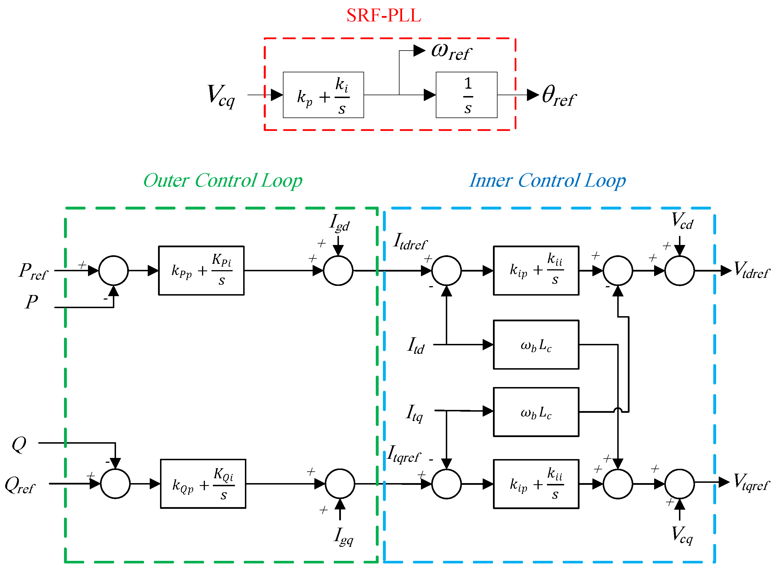
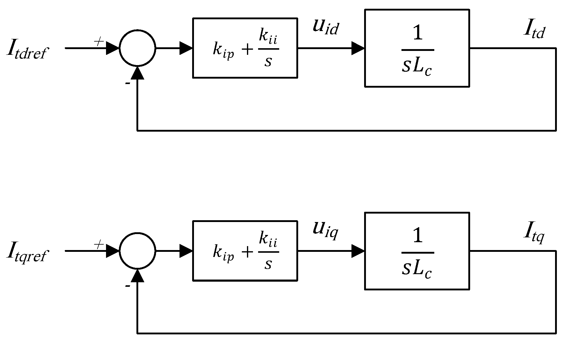
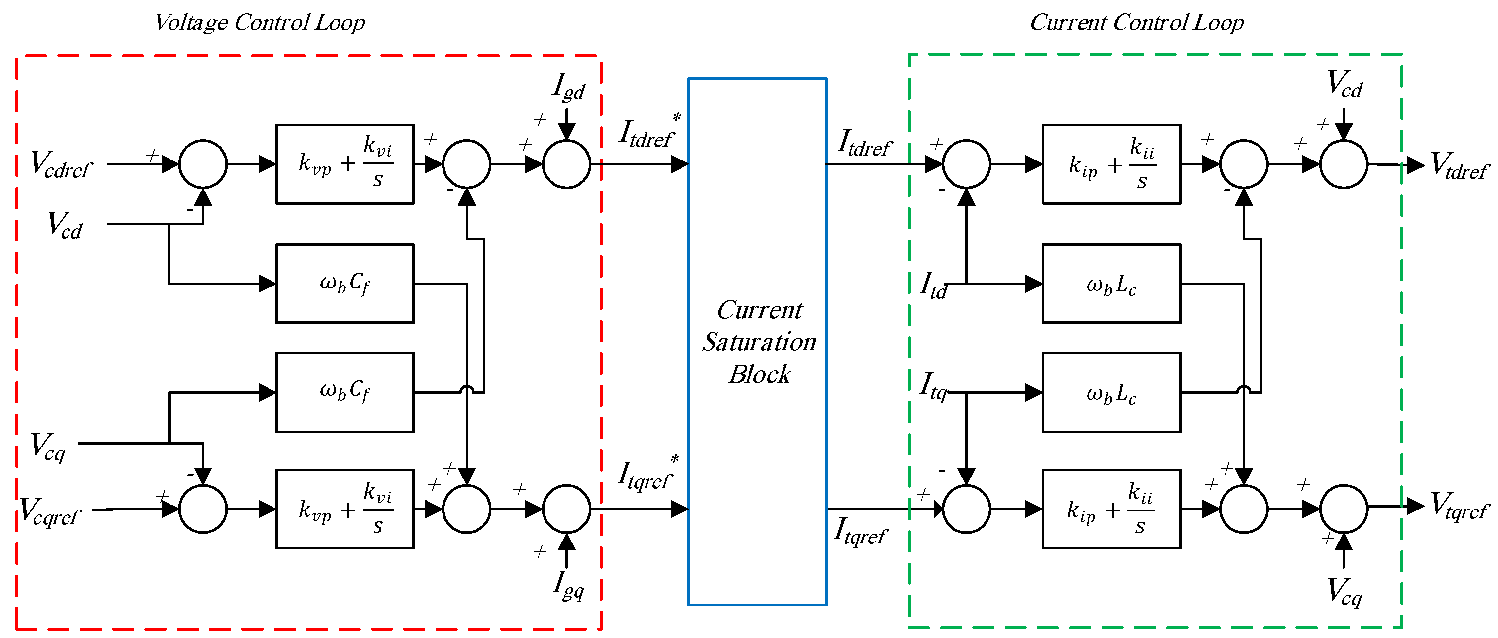
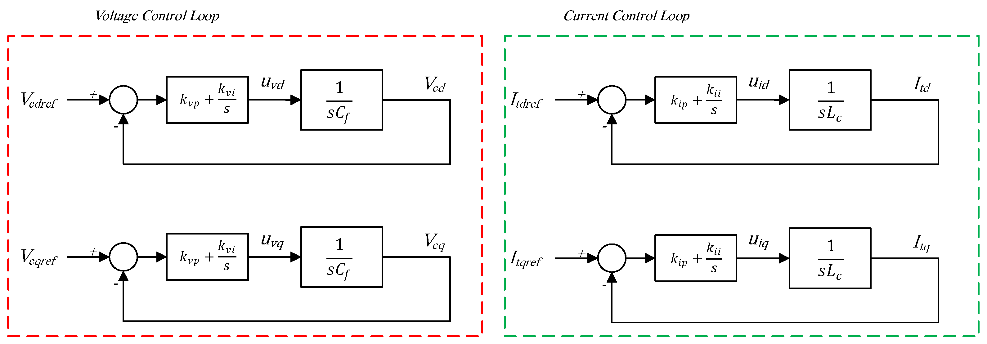
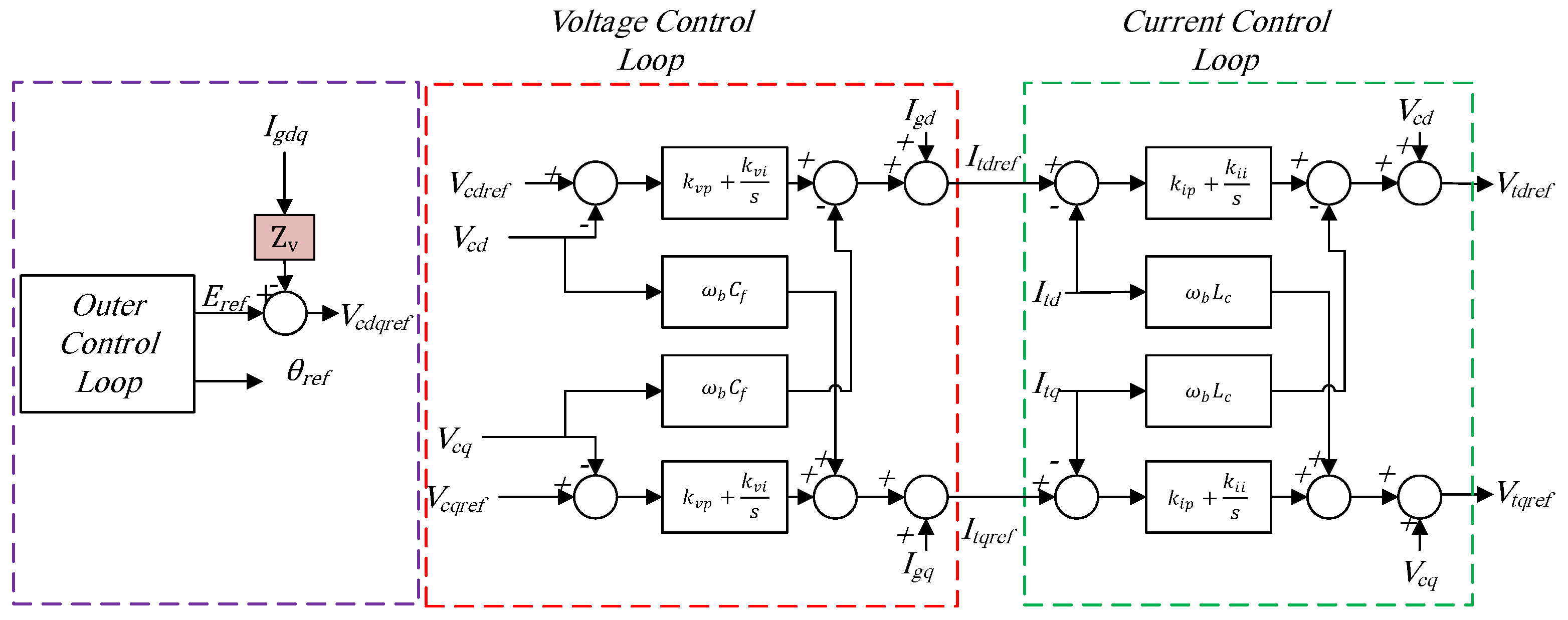
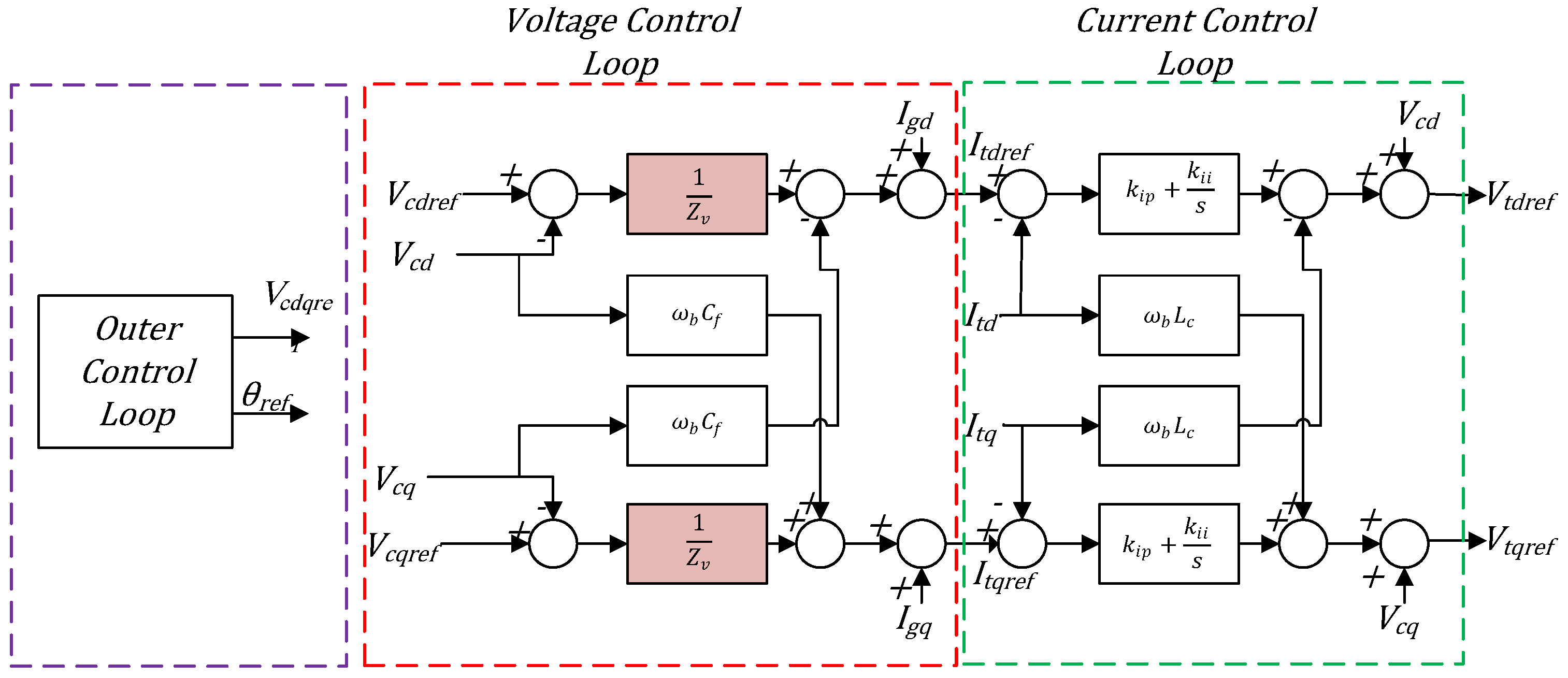
3.1. Inner Control Loops of GFMIs

After the references for the angle and the voltage magnitude of the PCC are generated by the outer control loop, they are fed into the inner control loops to generate the reference voltage at the inverter terminal. There are two main approaches for implementing inner control loops, namely, voltage-mode and current-mode; both are explained in the following sections.

3.1.1. Voltage-Mode Control

The block diagram of a typical voltage-mode controller for a GFMI is shown in Figure 7 [54]. In this method, $V_{cdqref}$, which is the output of the outer control loop, $V_{cdq}$, and two PI controllers are used to generate the reference terminal voltage of the inverter, $V_{tdqref}$. Then, this voltage and ${\theta }_{ref}$ are fed into a pulse-width modulation (PWM) generator to generate the switching pulses of the inverter.

Although simple in structure and design, the voltage-mode control method does not offer any output current control for the inverter, leading to overcurrent problems in the event of faults in the system [54].

3.1.2. Current-Mode Control

Current-mode control provides a solution to the overcurrent problem of voltage-mode control [54]. As shown in Figure 8, $V_{cdqref}$, which is the output of the outer control loop, $V_{cdq}$, and two PI controllers are used to generate the reference output current of the inverter, $I_{tdqref}$. Then, overcurrent protection schemes, such as saturation blocks, are implemented [1]. Various methods for implementing the current saturation block are reviewed in [56]. One of the typical methods is to set $I_{tdref}$ and $I_{tqref}$ to predefined values when the reference currents generated by the voltage control loop exceed a specific threshold [56]. $I_{tdqref}$ and $I_{tdq}$ are fed to two PI controllers to form the reference voltage for the inverter terminal, $V_{tdqref}$, which is then sent to a PWM generator [57,58].

The AC-side dynamics of the converter in this control scheme are shown in (5)–(8) [54], where, there are couplings between the d-axis and the q-axis dynamics of the voltage and current. To decouple the d-axis dynamics from the q-axis dynamics, feed-forward signals shown in Figure 8 are used [54].

$$L_c\frac{d{I}_{td}}{dt}=L_c{\omega }_{ref}{I}_{tq}+V_{td}-V_{cd},$$

(5)

$$L_c\frac{d{I}_{tq}}{dt}=-L_c{\omega }_{ref}{I}_{td}+V_{tq}-V_{cq},$$

(6)

$$C_f\frac{d{V}_{cd}}{dt}=C_f{\omega }_{ref}{V}_{cq}+I_{td}-I_{gq},$$

(7)

$$C_f\frac{d{V}_{cq}}{dt}=-C_f{\omega }_{ref}{V}_{cd}+I_{tq}-I_{gd}.$$

(8)

The simplified block diagram of the current-mode controller with the introduction of feed-forward signals is shown in Figure 9, and the dynamics of the controller are shown in (9)–(12).

$$L_c\frac{d{I}_{td}}{dt}=u_{id},$$

(9)

$$L_c\frac{d{I}_{tq}}{dt}=u_{iq},$$

(10)

$$C_f\frac{d{V}_{cd}}{dt}=u_{vd},$$

(11)

$$C_f\frac{d{V}_{cq}}{dt}=u_{vq}.$$

(12)

3.1.3. Virtual Impedance Method

As discussed in Section 2.2, GFMIs can be modeled as voltage sources [52]. When GFMIs are connected to strong grids, the small inductance connecting these two voltage sources together, makes the system prone to instability [18,59]. To improve the stability of the current-mode controlled GFMIs, the inner control loops are modified in some studies [18,58,60,61,62,63,64,65] using the virtual impedance method. The virtual impedance method helps to improve the performance of inverters by limiting the inverter’s current [60], decreasing the coupling of the output active and reactive power of the inverter, improving the power-sharing capability of the inverter [61,62], increasing system damping [63], and improving the converter stability considering different grid and transmission line conditions [18]. The virtual impedance method can result in different dynamics, as compared to conventional inner control, based on its application and control objective [64]. Two popular designs are referred to as “virtual impedance method” [18,58,60,61,62,63,64] and “virtual admittance method” [18,65]. These methods improve inverter stability by increasing the total inductance connecting the inverter to the grid [18].

In the virtual impedance method, as shown in Figure 10, the input to the voltage control loop is obtained by multiplying $I_{gdq}$ by the virtual impedance and subtracting it from the output of the outer control loop, $E_{ref}$ [64,65,66].

In the virtual admittance method, the PI controllers of the voltage control loop are replaced with the virtual admittance $\frac{1}{Z_v}$. The block diagram of the modified inner control loops is shown in Figure 11 [18,67]. Compared to the virtual impedance method, virtual admittance method provides a larger stability margin for the GFMI [18].

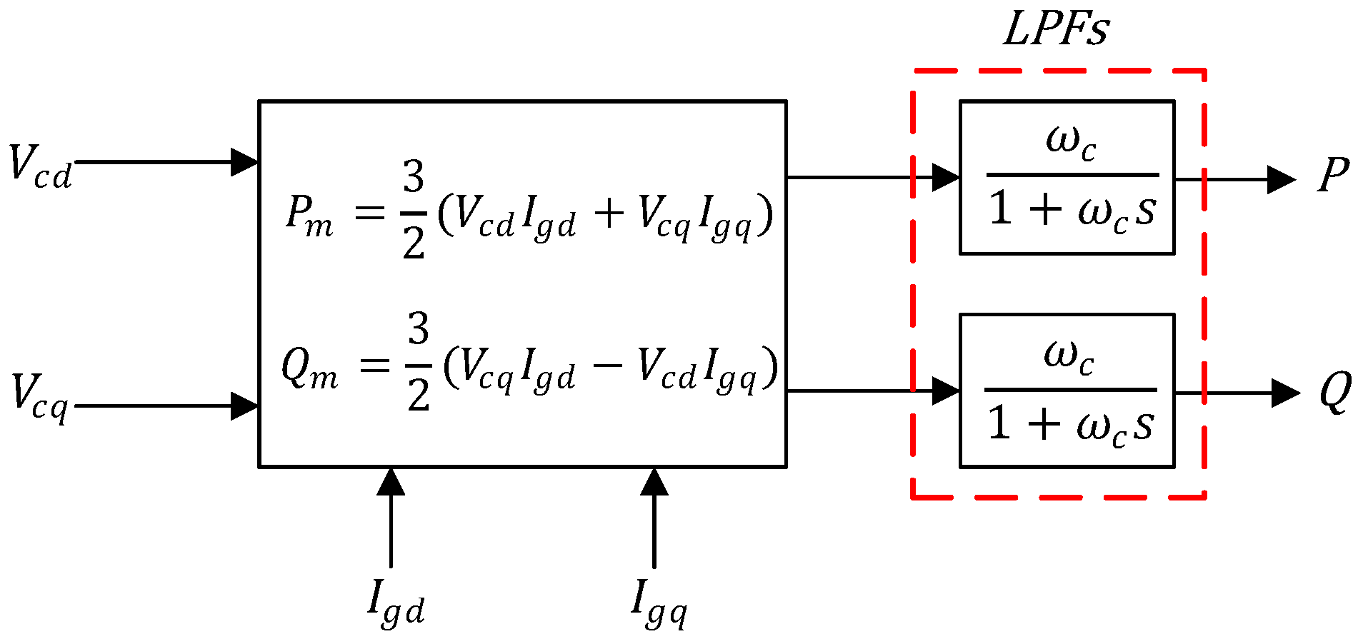
3.2. Outer Control Loop of GFMIs

In a two-bus system with a connecting transmission line with a large $\frac{X}{R}$ ratio, the active and reactive power transferred from bus 1 to bus 2 are as shown in (13) and (14), where $V_1$, $V_2$, R, X, and $\delta$ are the voltage magnitude at bus 1, voltage magnitude at bus 2, equivalent resistance and reactance of the transmission line connecting buses 1 and 2, and phase angle difference between buses 1 and 2 [68]. In (13) and (14), it is assumed that $\delta$ is small and $\frac{X}{R}$ is large. According to (13) and (14), the active power mainly depends on the angle difference between the bus voltages, and the reactive power depends on the voltage magnitudes [68]. This is true as the angle difference between two adjacent buses in a power system is mostly small, and transmission lines are also highly inductive.

$$P=\frac{V_1{V}_2}{X}sin\delta ,$$

(13)

$$Q=\frac{V_1^2-V_1{V}_{2}cos\delta }{X}.$$

(14)

Based on (13) and (14), the phase angle and the voltage magnitude at the grid-side of a GFMI can be regulated by controlling the output active and reactive power of the inverter, respectively, [1]. This is the basis for the operation of the outer controller of a GFMI. If $\frac{X}{R}$ ratio of the transmission line is low, the active and reactive powers will depend on the voltage magnitudes and the angle difference between the bus voltages, respectively, [1]. If X and R are comparable to each other, the multivariable transfer function of the active and reactive power should be used to relate them to the voltage magnitude and phase angle of the inverter terminal [1]. The output active and reactive power of the inverter are obtained as shown in Figure 12, where ${\omega }_c$ is the cut-off frequency of the filter.

The main control schemes introduced in the literature for GFMIs are presented in the following. In all of these schemes, the control depends on local measurements, and no communication is required between the inverters. A number of these control schemes provide inertia to support the grid dynamic response. Typically, inertia refers to the tendency of a physical object to resist change in its state of motion [69]. In power systems, rotors of SGs are in motion, and their mechanical speed is coupled with their electrical angular speed [69]. Therefore, the dynamics of their electrical angular speed can also represent the dynamics of their mechanical speed [69]. The swing equation of an SG, represents the dynamics of the rotor’s electrical angle and rotor’s electrical angular speed as shown in (15),

$$\frac{2H}{{\omega }_s}\frac{d^2\delta }{d{t}^2}+D\frac{d\delta }{dt}=P_m-P_e,$$

(15)

where H, ${\omega }_s$, $\delta$, D, $P_m$, $P_e$, and $\frac{d\delta }{dt}$ are the inertia constant, synchronous speed, angular position of the rotor with respect to a stationary axis, damping coefficient, mechanical power, electrical power, and electrical angular speed of the SG, respectively, [68]. H is the combined inertia constant of the generator and the turbine [68]. Since GFMIs have no moving parts, they cannot provide inertia unless their control schemes are designed to do so [69]. The inertia provided using this technique is called virtual inertia [69]. In this section, the ability of each control scheme in providing inertia will be discussed.

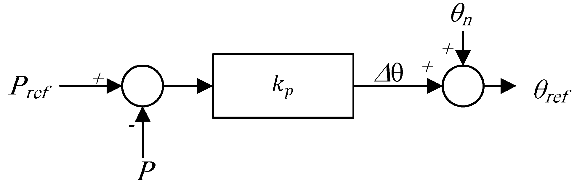
3.2.1. Frequency-Droop Control

In the frequency-droop control method, also known as droop control, the difference between $P_{ref}$ and P is multiplied by $k_p$, called the droop factor, and then added to ${\omega }_n$ to generate ${\omega }_{ref}$. By integrating ${\omega }_{ref}$, ${\theta }_{ref}$ is derived [32]. The block diagram of this method is shown in Figure 13. The angle dynamics in this control scheme are shown in (16).

$$\frac{1}{k_p}\frac{d{\theta }_{ref}}{dt}=\frac{{\omega }_n}{k_p}+P_{ref}-P.$$

(16)

It should be noted that an inertial term can be observed in (17) when considering the impact of LPFs of Figure 12 on the dynamic response of this scheme. Comparing (15) and (17), this scheme is unable to provide any tunable inertial response. The impacts of neglecting the effect of the low-pass filters (LPFs) on the dynamics of droop-controlled GFMIs are studied in [70,71].

$$\frac{1}{k_p{\omega }_c}\frac{d^2{\theta }_{ref}}{d{t}^2}+\frac{1}{k_p}\frac{d{\theta }_{ref}}{dt}=P_{ref}-P+\frac{{\omega }_n}{k_p}.$$

(17)

$V_{cdref}$, also referred to as $V_{ref}$ in the remainder of this paper, is generated by feeding the difference between $Q_{ref}$ and Q to a PI controller, with $k_{qp}$ and $k_{qi}$ as the proportional and integral gains, and then adding its output to $V_n$. $V_{cqref}$ is set to zero. The voltage dynamics are shown in (18).

$$V_{ref}=V_n+k_{qp}(Q_{ref}-Q)+k_{qi}\int (Q_{ref}-Q)dt.$$

(18)

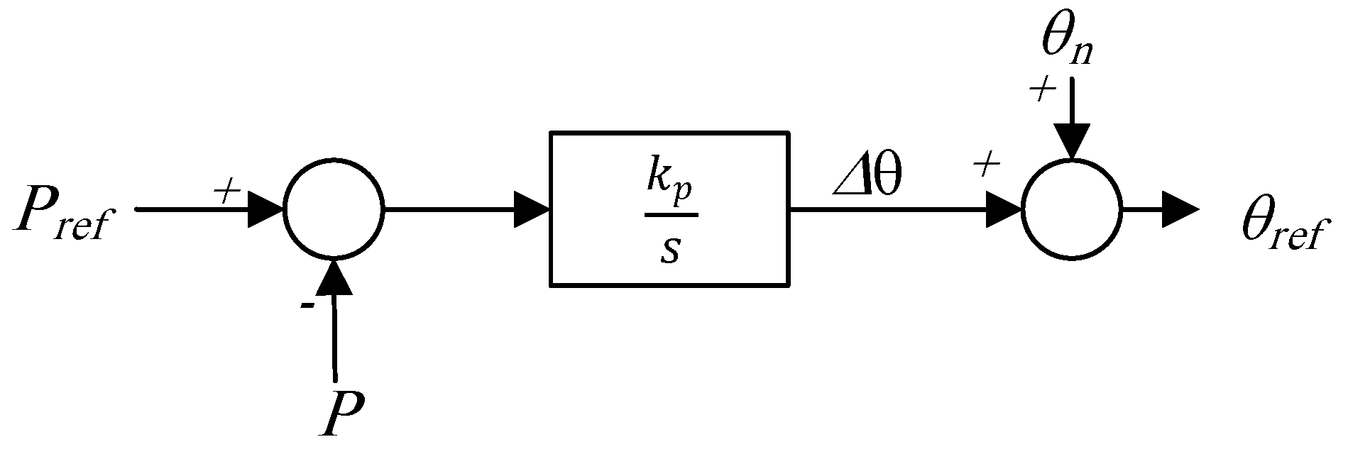
3.2.2. Angle-Droop Control

Similar to the frequency-droop control, in angle-droop control, ${\theta }_{ref}$ is generated by multiplying the difference between $P_{ref}$ and P by the droop factor, $k_p$, and adding the result to ${\theta }_n$ [33], as shown in Figure 14. The angle dynamics are shown in (19). This scheme does not provide virtual inertia. $V_{ref}$ is generated similar to that of the frequency-droop control scheme.

$${\theta }_{ref}=k_p(P_{ref}-P)+{\theta }_n.$$

(19)

3.2.3. Power Synchronization Control (PSC)

As shown in Figure 15, this method is quite similar to the frequency-droop control. The difference between $P_{ref}$ and P is multiplied by $k_p$ and then integrated to form $\mathsf{\Delta }\theta$. $\mathsf{\Delta }\theta$ is added to ${\theta }_n$ to generate ${\theta }_{ref}$ [34]. The angle dynamics of this method are shown in (20). Considering the impact of LPFs on the dynamics of this scheme, this scheme provides virtual inertia. $V_{ref}$ is generated similar to the previous schemes.

$$\frac{1}{k_p}\frac{d{\theta }_{ref}}{dt}=P_{ref}-P.$$

(20)

3.2.4. Synchronverter

The basis for controlling a GFMI as a synchronverter is to emulate the dynamics of an SG [1,30,35]. The dynamics of this control scheme are shown in (21)–(24)

$$\frac{d^2{\theta }_{ref}}{d{t}^2}+\frac{D_p}{J}\frac{d{\theta }_{ref}}{dt}=\frac{1}{J}(T_m-T_e),$$

(21)

$$T_e=M_f{i}_f\langle i_t,\left[\begin{array}{c}sin\left({\theta }_{ref}\right)\\ sin({\theta }_{ref}-\frac{2\pi }{3})\\ sin({\theta }_{ref}+\frac{2\pi }{3})\end{array}\right]\rangle ,$$

(22)

$$V_{tref}=\omega M_f{i}_f\left[\begin{array}{c}sin\left({\theta }_{ref}\right)\\ sin({\theta }_{ref}-\frac{2\pi }{3})\\ sin({\theta }_{ref}+\frac{2\pi }{3})\end{array}\right],$$

(23)

$$Q=-\omega M_f{i}_f\langle i_t,\left[\begin{array}{c}cos\left({\theta }_{ref}\right)\\ cos({\theta }_{ref}-\frac{2\pi }{3})\\ cos({\theta }_{ref}+\frac{2\pi }{3})\end{array}\right]\rangle .$$

(24)

where $T_m$, $T_e$, $M_f{i}_f$, J, $D_p$, and $D_q$ are the virtual mechanical torque, virtual electrical torque, virtual mutual flux, moment of inertia, damping coefficient, and voltage droop coefficient, respectively, [30,35]. $\langle .,.\rangle$ denotes the inner product. The block diagram of this scheme is shown in Figure 16, where K is the reactive power integrator gain.

Equation (21) shows that this scheme provides virtual inertia. In this scheme, $Q_{ref}$ is compared with Q and integrated; then, it is added to the voltage droop signal to generate the virtual mutual flux. Using this scheme, the reference for inverter terminal voltage is directly generated in the same way the back electromotive force is generated in an SG; thus, there is no need for inner control loops [1,30,35].

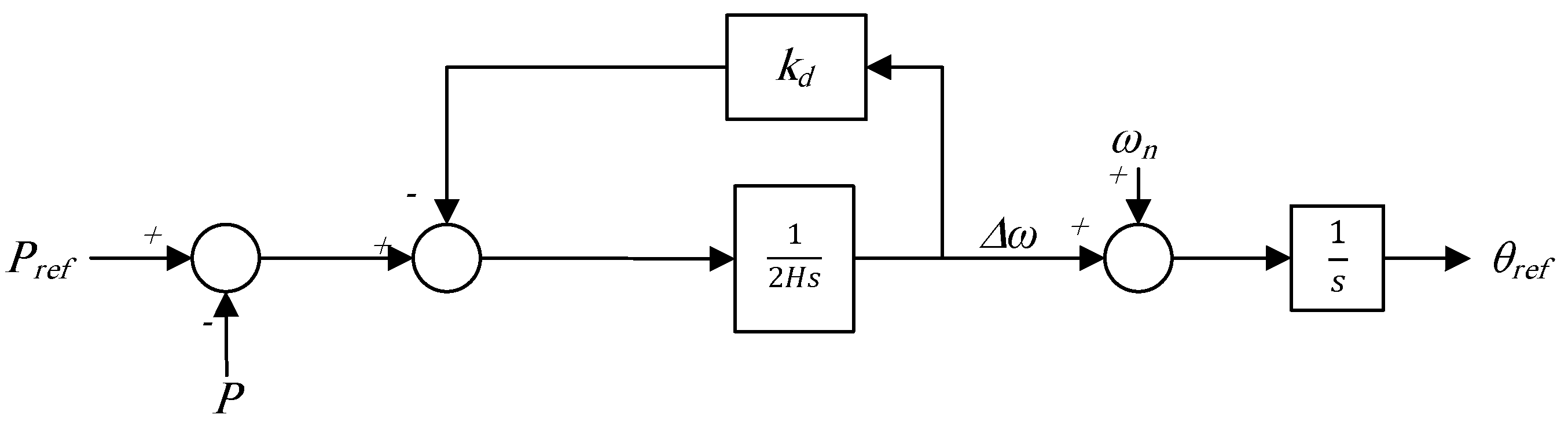
3.2.5. Virtual Synchronous Machine (VSM)

In order to emulate the dynamic response of an SG and to provide inertia in case of a grid disturbance, the VSM aims to mimic the swing equation of an SG, which is shown in (15). The block diagram of this scheme is shown in Figure 17 [36,37].

The angle dynamics are shown in (25),

$$2H\frac{d^2{\theta }_{ref}}{d{t}^2}+k_d\frac{d{\theta }_{ref}}{dt}=k_d{\omega }_n+P_{ref}-P,$$

(25)

where H and $k_d$ are the inertia constant and the damping coefficient, respectively. (25) shows that this scheme provides virtual inertia. $V_{ref}$ is generated using a PI controller, as shown in Figure 13.

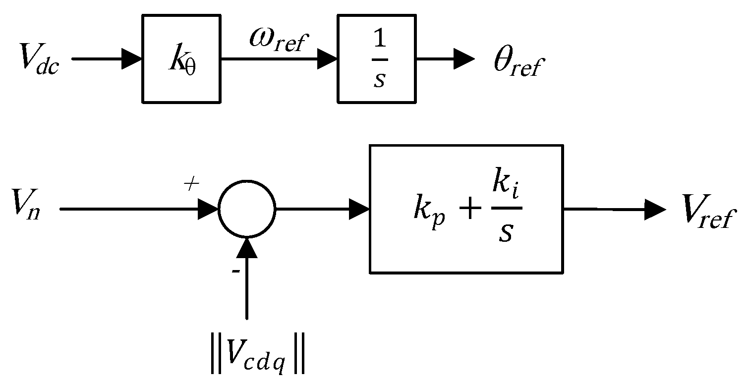
3.2.6. Matching Control

The DC-side dynamics of a GFMI are shown in (26),

$$C_{dc}\frac{d{V}_{dc}}{dt}+\frac{1}{R_{dc}}{V}_{dc}=I_{dcref}-i_{dc},$$

(26)

where $C_{dc}$, $V_{dc}$, $I_{dcref}$, $R_{dc}$, and $i_{dc}$ are the capacitance of the DC link, DC link voltage, DC-side reference current, DC-side resistance modeling the losses, and the input current of the inverter, respectively. Another form of the swing equation of an SG is shown in (27),

$$J\frac{d^2\delta }{d{t}^2}+D_d\frac{d\delta }{dt}=T_m-T_e,$$

(27)

where J, $D_d$, $T_m$, and $T_e$ are the moment of inertia, damping torque coefficient, mechanical torque, and electrical torque. By comparing (26) and (27), one can realize the duality between $T_m$ and $T_e$, as well as $I_{dcref}$ and $i_{dc}$. References [38,39,40] used this duality as the basis of the matching control scheme. The main idea behind this control method is that by using the DC-side dynamics, the dynamics of the GFMI can be exactly matched to those of an SG. Therefore, this scheme is called matching control. Matching control uses the DC link voltage to control the phase angle of the GFMI, as shown in Figure 18 [50,51,54].

The dynamics of matching control are shown in (28) and (29),

$$\frac{d{\theta }_{ref}}{dt}=k_{\theta }{V}_{dc},$$

(28)

$$V_{ref}=k_p(V_n-\parallel V_{cdq}\parallel )+k_i\int (V_n-\parallel V_{cdq}\parallel )dt,$$

(29)

where $k_{\theta }=\frac{{\omega }_n}{V_{dcn}}$ is the frequency gain. $V_{dcn}$ is the nominal DC-link voltage, and $k_p$ and $k_i$ are proportional and integral gains of the voltage controller used in the outer control loop. Considering (26) and (28), this scheme provides virtual inertia.

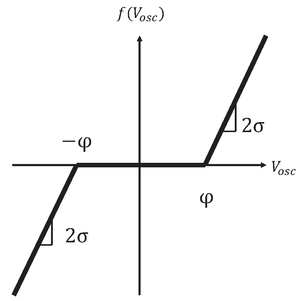
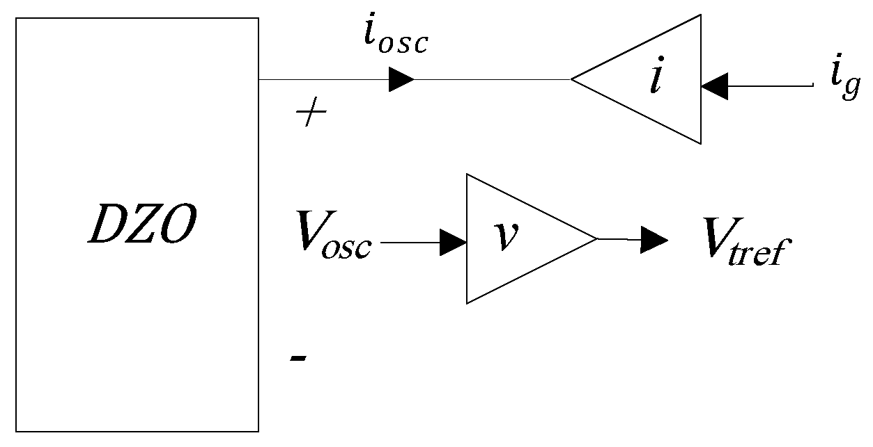
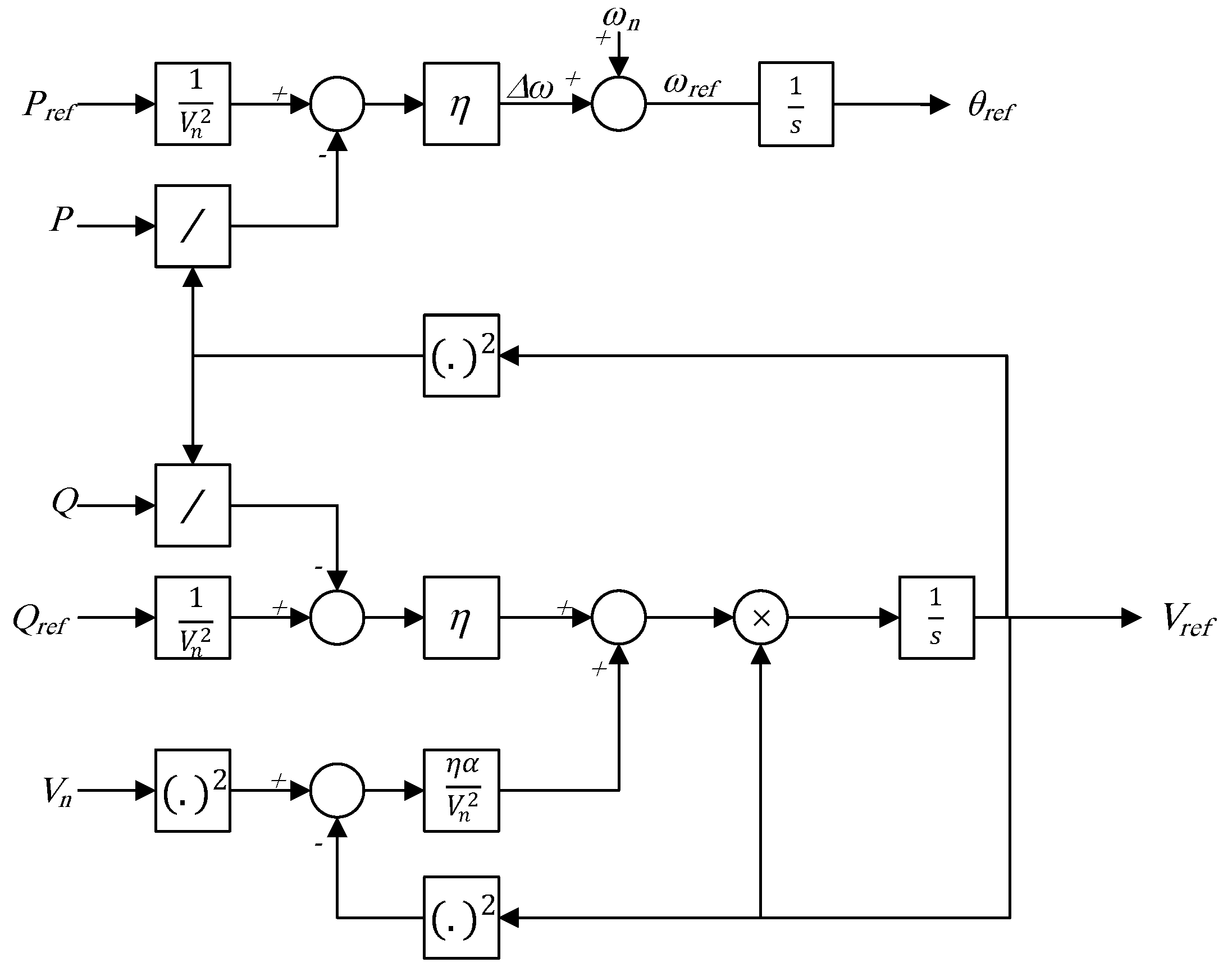
3.2.7. Virtual Oscillator Control (VOC)

Unlike parallel SGs, load sharing and synchronization in a system with parallel inverters is not easily achieved [72]. This is due to the fact that control schemes of converters, and not their physical characteristics, determine their dynamics [72]. To achieve load sharing and synchronization in systems with parallel GFMIs, a dead-zone oscillator (DZO) control scheme can be used [73]. Furthermore, controlling a GFMI as a virtual oscillator ensures a sinusoidal output voltage [72]. A DZO circuit is shown in Figure 19 [73], where R, C, and L are the DZO resistor, capacitor, and inductor, respectively. $V_{osc}$, $i_{osc}$, and $i_L$ are the voltage and current of the DZO, and its inductor current, respectively.

The dynamics of the voltage-dependent current source in this circuit, $i_o\left(V_{osc}\right)$, is shown in (30),

$$i_o\left(V_{osc}\right)=f\left(V_{osc}\right)-\sigma V_{osc},$$

(30)

where $f\left(V_{osc}\right)$ is a dead-zone function, shown in Figure 20, and (31), where $\sigma$, and $\phi$ are parameters of $f\left(V_{osc}\right)$ [73].

$$f\left(V_{osc}\right)=\left\{\begin{array}{cc}2\sigma (V_{osc}-\phi )\hfill & \phi \le V_{osc}\hfill \\ 0\hfill & -\phi \le V_{osc}\le \phi \hfill \\ 2(\sigma V_{osc}+\phi )\hfill & V_{osc}\le -\phi \hfill \end{array}\right..$$

(31)

The dynamics of the DZO are shown in (32) and (33) [73].

$$\frac{d{V}_{osc}}{dt}=\frac{1}{C}[V_{osc}(\sigma -\frac{1}{R})-f\left(V_{osc}\right)-i_L-i_{osc}],$$

(32)

$$\frac{d{i}_L}{dt}=\frac{1}{L}{V}_{osc}.$$

(33)

Reference [73] shows that in order to have approximately a sinusoidal waveform for $V_{osc}$, $\sqrt{\frac{L}{C}}(\sigma -\frac{1}{R})\ll 1$. The control loop of the VOC scheme is shown in Figure 21 [41]. Scaling gains v and i provide output voltage and currents in the same scale as those of a GFMI. In this control scheme, the reference voltage at the inverter terminal is generated without using inner control loops [41,74].

A sufficient condition for the synchronization of any number of parallel VOC GFMIs is shown in (34), where $Z_{fr}$ is the reference output filter impedance [75].

$$\underset{\omega \in \mathbb{R}}{sup}\parallel \frac{{\left(vi\right)}^{-1}{Z}_{fr}\left(j\omega \right)Z_{osc}\left(j\omega \right)}{{\left(vi\right)}^{-1}{Z}_{fr}\left(j\omega \right)+Z_{osc}\left(j\omega \right)}\parallel \sigma <1.$$

(34)

For the $j^{th}$ GFMI, the output filter impedance is $k_j^{-1}{Z}_{fr}$, where $k_j$ is an output scaling parameter to ensure power sharing capability [72]. The relative power of parallel VOC GFMIs are shown in (35) [72].

$$\frac{P_k}{P_j}=\frac{k_j}{k_k}.$$

(35)

The power set-points of the inverter, $P_{ref}$ and $Q_{ref}$, are not directly used in this control scheme to set its output voltage reference. To overcome this issue, the dispatchable virtual oscillator control (dVOC) method is introduced in [76]. The dynamics of this scheme in $\alpha \beta$ coordinates are shown in (36)–(39) [42].

$$\frac{d{V}_{ref\alpha \beta }}{dt}={\omega }_n\mathit{M}{V}_{ref\alpha \beta }+\eta (K{V}_{ref\alpha \beta }-R_2\left(k\right)i_{g\alpha \beta })+\eta \frac{\alpha }{V_n^2}(V_n^2-\parallel V_{ref\alpha \beta }^2\parallel \left)\right),$$

(36)

$$R_2\left(k\right)=\left[\begin{array}{cc}cos\left(k\right)& -sin\left(k\right)\\ sin\left(k\right)& cos\left(k\right)\end{array}\right],$$

(37)

$$K=\frac{1}{V_n^2}{R}_2\left(k\right)\left[\begin{array}{cc}{P}_{ref}& Q_{ref}\\ -Q_{ref}& P_{ref}\end{array}\right],$$

(38)

$$M=\left[\begin{array}{cc}0& -1\\ 1& 0\end{array}\right],$$

(39)

where $k=arctan\left(\frac{X_g}{R_g}\right)$, and $X_g$ and $R_g$ are transmission line reactance and resistance, respectively. $\eta$ and $\alpha$ are synchronization and amplitude regulation gains, respectively, [77]. Matrix M is the ${90}^{\circ }$ rotation matrix [77]. Parameter k corresponds to the dynamics of transmission lines, where $k=0$ for fully resistive lines and $k=\frac{\pi }{2}$ for fully inductive lines [76]. $i_{g\alpha \beta }$ and $V_{ref\alpha \beta }$ are the inverter grid-side current and the reference voltage for the PCC in $\alpha \beta$ coordinates, respectively.

As shown in (36), the dynamics of a dVOC do not explicitly match with the dynamics of a VOC [77]. The dynamics of (36) consists of three terms. The first term, ${\omega }_n\mathit{M}{V}_{ref\alpha \beta }$, generates a sinusoidal voltage, $V_{ref\alpha \beta }$, with the nominal angular frequency of ${\omega }_n$. The second term, $\eta (K{V}_{ref\alpha \beta }-R_2\left(k\right)i_{g\alpha \beta })$, corresponds to tracking the power set-points, $P_{ref}$ and $Q_{ref}$ by minimizing the phase difference between $i_{g\alpha \beta }$ and the reference current shown by $K{V}_{ref\alpha \beta }$. The last term, $\eta \frac{\alpha }{V_n^2}(V_n^2-\parallel V_{ref\alpha \beta }^2\parallel \left)\right)$, minimizes the voltage magnitude error [77].

For a dVOC GFMI connected to a fully inductive transmission line, Equation (36) can be rewritten in the form of (40) and (41), in the dq coordinates [78]. The block diagram of dVOC scheme for a GFMI connected to a fully inductive transmission line is shown in Figure 22 [78]. As shown in Figure 22 and (40) and (41), in the dVOC scheme, active and reactive power references of the converter are used directly to control P and Q. Equation (40) shows that this scheme does not provide virtual inertia.

$$\frac{d{\theta }_{ref}}{dt}={\omega }_n+\eta (\frac{P_{ref}}{V_n^2}-\frac{P}{V_{ref}^2}),$$

(40)

$$\frac{d{V}_{ref}}{dt}=\eta (\frac{Q_{ref}}{V_n^2}-\frac{Q}{V_{ref}^2})V_{ref}+\frac{\eta \alpha }{V_n^2}(V_n^2-V_{ref}^2)V_{ref}.$$

(41)

3.2.8. Summary

In this section, inner and outer control loops of GFMIs were discussed. Voltage-mode and current-mode control are two conventional methods for implementing inner control loops of a GFMI, while voltage-mode control contains a single control loop and has a simple design, it does not provide overcurrent protection for the inverter. The current-mode control consists of voltage and current control loops, which makes overcurrent protection possible. Virtual impedance and virtual admittance methods and their impact on the stability of GFMIs were also discussed in this section. Different outer control loop schemes, such as frequency-droop control, angle-droop control, PSC, synchronverter control, VSM control, matching control, VOC, and dVOC schemes were also reviewed. No communication between parallel GFMIs in any of the control schemes discussed in this paper is required. Frequency-droop control, PSC, synchronverter, VSM, and matching control schemes provide virtual inertia; however, the inertia provided by frequency-droop control and PSC schemes is not tunable as they provide an inertial response considering the dynamics of LPFs. Synchronverter and VOC schemes offer no overcurrent protection. VOC scheme provides a fast response as there is no need for any transformation between different coordinates in this scheme. However, the output power of VOC GFMIs cannot be dispatched [1,29]. Although dVOC scheme offers a solution to the dispatchability problem of VOC scheme, it is a new scheme with a complex design [29]. The comparison between the aforementioned control schemes is presented in

Table 2. Comparison between different GFMI control schemes.

Control Scheme	Tunable Virtual Inertia	Current Limiting Capability	Dispatchability
Frequency-droop	No	Yes	Yes
Angle-droop	No	Yes	Yes
PSC	No	Yes	Yes
Synchronverter	Yes	No	Yes
VSM	Yes	Yes	Yes
Matching Control	Yes	Yes	Yes
VOC	No	No	No
dVOC	No	Yes	Yes

. It is important to note that other control schemes for GFMIs are introduced in the literature, such as configurable natural droop [1,43], generalized droop [1,44], unified voltage oscillator [1,45], $H_{\infty }\setminus H_2$-based robust fixed-structure [1,46,47], and frequency shaping-based [1,48]. However, this paper only focuses on the control schemes that have been considered in the existing literature for stability analysis of GFMIs.

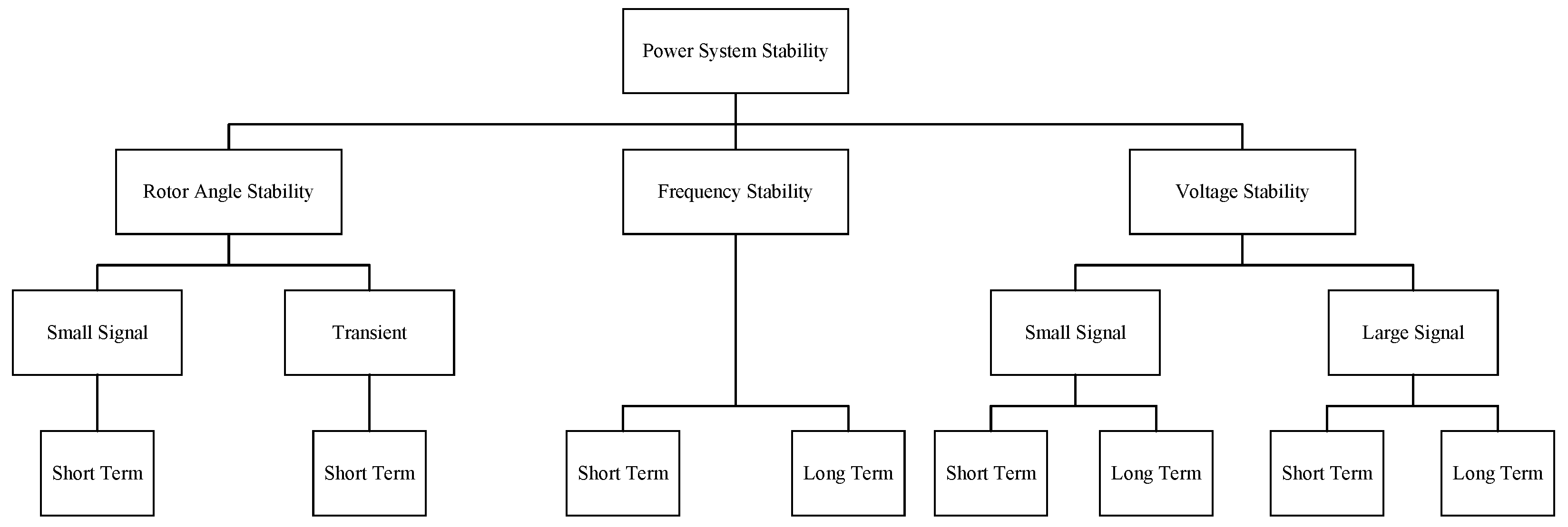
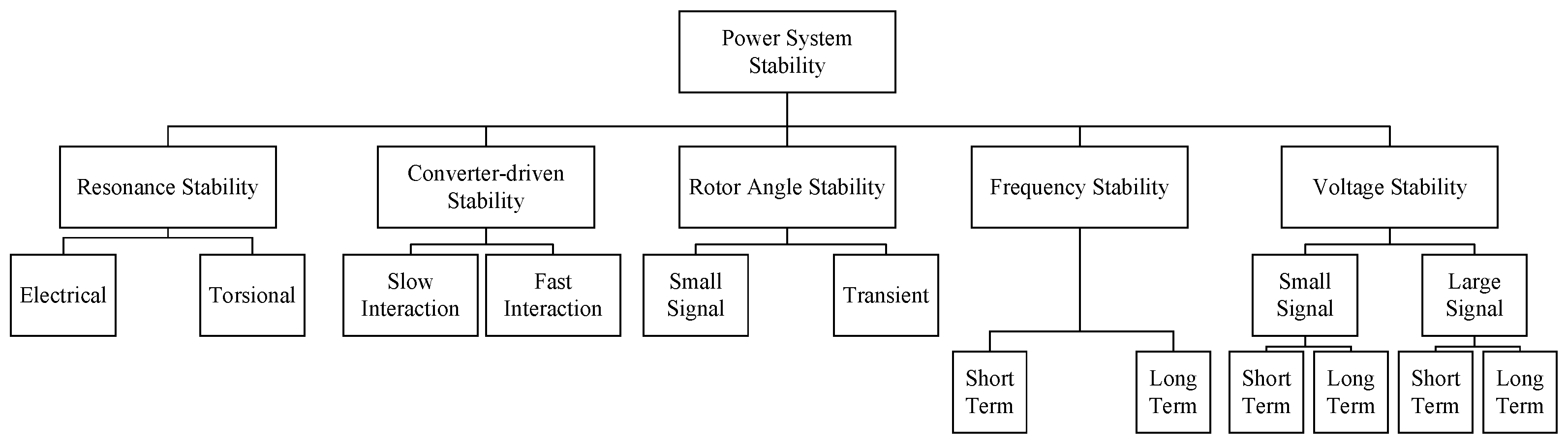
4. Stability of GFMIs

Power system stability is a well-established concept defined as the ability of a power system to operate at a state of equilibrium under normal conditions and to recover to an acceptable state of equilibrium after a disturbance [79]. Power system stability is classified into three main categories: frequency stability, voltage stability, and rotor angle stability, as shown in Figure 23 [80]. Frequency stability is the ability of a power system to maintain a steady frequency after an imbalance between generation and load [80]. Voltage stability is the ability of a power system to sustain steady, acceptable voltages at all system buses, both during regular operation and following a disturbance [79]. Rotor angle stability is the ability of SGs in a power system to maintain synchronism [79]. Large signal and small signal categories shown in Figure 23 correspond to the ability of the system to remain stable after large and small disturbances, respectively, [80].

The conventional classification of power system stability presented in Figure 23, is based on the dominance of SGs, and is inadequate for power grids with large integration of power electronic converters. These converters, found in wind and photovoltaic generation units, energy storage systems, HVDC systems, flexible AC transmission systems, and power electronic-interfaced loads, introduce fast dynamics to the power grid [7,8]. A revised classification of power system stability, considering the impact of power electronic converters, is proposed in [81], and presented in Figure 24. In [81], two new categories, i.e., resonance stability and converter-driven stability are introduced [81].

When oscillatory energy exchange between specific system components leads to a significant increase in voltages, currents, or torques above a predefined threshold, it triggers a resonance stability event [59]. Resonance stability is classified into torsional and electrical categories [81]. In order to define torsional and electrical resonance stability, the definitions of subsynchronous oscillation and subsynchronous resonance (SSR) are required [81]. Subsynchronous oscillation corresponds to an electric power system where there is notable energy exchange between the electrical network and a turbine-generator at the natural frequency of the turbine-generator following a disturbance [82]. The frequency of such oscillations is less than the synchronous frequency of the system [82]. SSR is a resonance related to the oscillatory characteristics of electrical and mechanical variables of a turbine-generator when connected to a series compensated transmission line [82]. In SSR, the subsynchronous oscillations can be lightly damped, undamped, or even negatively damped [82].

A torsional resonance is a type of SSR wherein the turbine-generator shaft experiences torsional oscillations due to a significant energy exchange between the shaft and the electrical network [83]. The interactions between fast-acting power electronic converters and nearby turbine-generators can trigger torsional SSR events [81,82,84,85,86,87,88].

Electrical resonance stability corresponds to a type of SSR when an oscillatory energy exchange takes place between the series compensated transmission lines and a generator due to the generator electrical characteristics [81]. Electrical resonance stability for variable speed induction generators of doubly-fed induction generators (DFIGs) was studied for the first time in 2003 [81,89]. An electrical resonance might happen between the DFIG and the series compensated transmission line when a DFIG is directly connected to the grid. At subsynchronous frequencies, the net apparent resistance of this circuit is negative which leads to a large oscillatory energy exchange between the series capacitor of the compensated transmission line and the effective inductance of the induction generator [81]. Electrical resonance stability issues in a real-world power grid were reported for the first time in 2009 in the Electric Reliability Council of Texas (ERCOT) [81,86,90,91,92]. Similar electrical resonance stability issues have happened in the Xcel Energy network in Minnesota, US [81,93].

Dynamics of different phenomena in a power system cover a wide range, from 1 $\mathsf{\mu }$s timescale of lightning propagation to 10⁴ s timescale of boiler dynamics [81]. Dynamics of power electronic converters cover a wide range of frequencies. For example, converter outer control loops have an operating frequency range of 1–10 Hz and converter switching frequency is in the kHz range [54]. This wide frequency range leads to interactions between converter control dynamics and various dynamics of power systems, such as electromechanical dynamics of machines, dynamics of nearby converters, and electromagnetic transients of the network, leading to various oscillations in the power network [81,94]. The oscillatory events due to these interactions are categorized under converter-driven stability.

Fast-interaction converter-driven stability events can be the result of interactions between fast inner control loops of converters and passive components of the system causing high-frequency oscillations [81,95,96]. High-frequency switching of converters can also cause high-frequency resonances with LCL power filters, causing a fast-interaction converter-driven stability issue [81,95,97]. The interactions between controllers of nearby converters can also cause high-frequency oscillations classified under fast-interaction converter-driven stability category [81,98,99]. Interactions between outer control loops of power electronic converters and slow-response components of the power network, such as electromechanical dynamics of SGs, are categorized under slow-interaction converter-driven stability. Studies of [81,100,101,102,103] show that the system strength at the connection point of converters affects these low-frequency oscillations. Interactions between direct-drive permanent magnet generators of wind turbines and weak AC grids has resulted in low-frequency oscillations and slow-interaction converter-driven instability issues in Xinjiang, China, since 2014 [81,103,104]. The rating of converters and their control strategies are among the factors that affect slow-interaction converter-driven stability [81,100].

It is important to note that stability categories of Figure 24 and their definitions are based on GFLI control schemes, and GFMI control schemes and their impact on these categories have not been addressed in [81]. In the existing literature, small-signal stability and transient stability are the main categories of stability associated with GFMIs, as shown in Figure 25 [1]. Definitions of small-signal and transient stability for GFMIs, stability analysis tools, and existing studies on the stability of GFMIs are presented in the following sections.

4.1. Small-Signal Stability

The power system’s ability to keep its synchronism under small disturbances is called small-signal stability [79]. Assume that the dynamic equations of the system under study form a set of first-order nonlinear differential equations in the state-space form as shown in (42) [79].

$$\begin{array}{cc}\hfill & \dot{x}=f(x,u),\hfill \\ \hfill & y=g(x,u).\hfill \end{array}$$

(42)

After linearizing the system of (42) using Taylor series expansion, the small-signal state-space model of the system is derived, as shown in (43). Based on the small-signal model of the system, three main methods are used to analyze system small-signal stability: eigenvalue analysis, impedance-based analysis, and robust stability analysis.

$$\begin{array}{cc}\hfill & \mathsf{\Delta }\dot{x}=A\mathsf{\Delta }x+B\mathsf{\Delta }u,\hfill \\ \hfill & \mathsf{\Delta }y=C\mathsf{\Delta }x+D\mathsf{\Delta }u.\hfill \end{array}$$

(43)

4.1.1. Eigenvalue Analysis

Using the eigenvalues of A, small-signal stability of the system can be analyzed by Lyapunov’s first method; if all eigenvalues have negative real parts, the system is stable. Otherwise, either the system is unstable (there is at least one eigenvalue with a positive real part) or its stability cannot be studied using this method [79]. Sensitivity analysis is used for studying the sensitivity of the eigenvalues of A to each of its elements [79]. Participation factors are used to determine the relative participation of different states of the system in system’s different modes [79]. One of the main disadvantages associated with this method is that the complete model of the system must be known [105].

4.1.2. Impedance-Based Analysis

Small-signal stability analysis of a system can be performed using the impedance-based method. As an example, in this method for a GFMI connected to a grid, the Thevenin equivalent circuit of each of these systems is derived [106]. In Figure 26, $V_{th1}$, $V_{th2}$, $Z_{th1}$, $Z_{th2}$, and I are the equivalent Thevenin voltage of the GFMI, equivalent Thevenin voltage of the grid, equivalent Thevenin impedance of the GFMI, equivalent Thevenin impedance of the grid, and current flowing to the grid from the GFMI. Current I can be formulated as shown in (44) and (45) [106].

$$I\left(s\right)=H\left(s\right)(V_{th1}\left(s\right)-V_{th2}\left(s\right)),$$

(44)

$$H\left(s\right)=\frac{Z_{th2}{\left(s\right)}^{-1}}{1+\frac{Z_{th1}\left(s\right)}{Z_{th2}\left(s\right)}}.$$

(45)

Transfer function $H\left(s\right)$ resembles the transfer function of a closed loop system with the open loop gain of $Z_{th2}{\left(s\right)}^{-1}$ and the negative feedback gain of $Z_{th1}\left(s\right)$. If $\frac{Z_{th1}\left(s\right)}{Z_{th2}\left(s\right)}$, the return-ratio matrix of the system, satisfies the Nyquist criterion and both $V_{th1}\left(s\right)$ and $V_{th2}\left(s\right)$ are stable, this system will be stable [106]. Passivity theory provides another sufficient condition for stability of the system of Figure 26, shown in (46) [106]. $Z_{thi}$ is the equivalent Thevenin impedance of the ith source.

$$Re\left(Z_{thi}\left(j\omega \right)\right)>0,\forall \omega \in (0,+\infty ),i=1,2.$$

(46)

This method allows for modeling different parts of the system with a black-box approach, as it only needs the equivalent Thevenin model of the two subsystems and does not require the detailed model of system components [105].

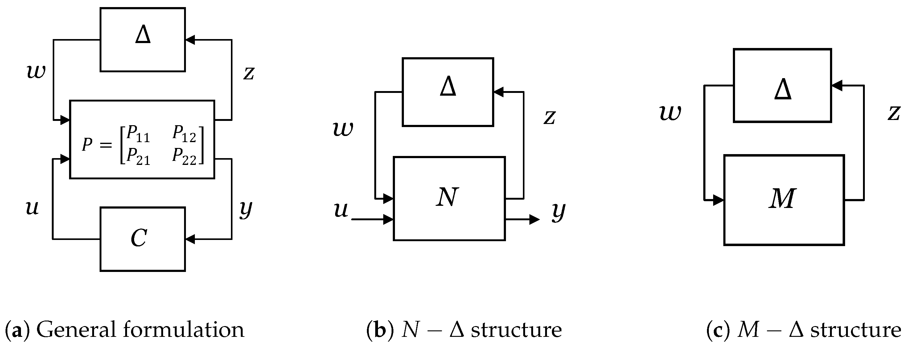
4.1.3. Robust Stability Analysis

In order to ensure system stability when there are uncertainties in the system, robust stability analysis is used. The lower fractional transformation (LFT) is used to study the robust stability of the system shown in Figure 27a [107,108], where w, u, y, and z are, respectively, the exogenous input, control input, measured output, and regulated output and P, C, and $\mathsf{\Delta }$ represent the transfer functions of the system, controller and perturbation, respectively. Rearranging the system of Figure 27a will result in the $N-\mathsf{\Delta }$ structure of Figure 27b, where N is obtained via (47) [107].

$$N\triangleq P_{11}+P_{12}C{(I-P_{21}C)}^{-1}{P}_{21}.$$

(47)

To analyze robust stability of the system, the system can be rearranged into the $M-\mathsf{\Delta }$ structure of Figure 27c, where $M=N_{11}$ is the transfer function from z to w [107,109]. The $\mu$ factor is defined in (48). The $\mu$ factor is the structured singular value of M. $\mu \left(M\right)$ can be calculated for any given M, by searching through stable perturbations $\mathsf{\Delta }$ and finding the reciprocal of the smallest $\overline{\sigma }$, maximum singular value, making $det(I-M\mathsf{\Delta })=0$ [109]. The inverse of $\mu$ factor is used as a measure of stability margin for analyzing robust stability of systems [107].

$$\mu \left(M\right)\triangleq \frac{1}{\underset{\mathsf{\Delta }}{min}\left\{\overline{\sigma }\right|det(I-M\mathsf{\Delta })=0\}}$$

(48)

4.1.4. Small-Signal Stability of GFMIs

The small-signal stability studies of GFMIs in the literature use eigenvalue analysis, impedance-based analysis, or robust stability analysis. These studies for various control schemes are reviewed in the following sections.

Droop Control Scheme

Reference [70] studies the impact of LPFs in the outer control loops of two droop-controlled GFMIs, connected in parallel and supplying a constant current load, on the small-signal stability of the system by using eigenvalue plots. It is concluded that LPFs increase the damping of the overall system response. Reference [110] examines the small-signal stability of a grid-connected droop-controlled GFMI. The impacts of the proportional gains of the voltage and current control loops on the stability margin of the system are studied using eigenvalue plots and participation factor calculation. It is revealed that the proportional gain of the PI controllers of the voltage control loop has a greater impact on small-signal stability of GFMIs compared to that of the current control loop. Reference [59] studies small-signal stability of voltage-mode and current-mode droop-controlled GFMIs. The system under study consists of two parallel droop-controlled GFMIs supplying a load in the islanded mode. The stability margins of these two control methods are compared to each other using eigenvalue plots. It is concluded that the voltage-mode control scheme leads to a larger stability margin compared to the current-mode scheme.

Reference [18] studies the effect of the virtual impedance on small-signal stability of a droop-controlled grid-connected GFMI. The stability margins of conventional droop control, virtual impedance, and virtual admittance methods are compared with each other using eigenvalue plots. The impact of the magnitude and phase of the virtual admittance on the stability margin is also investigated. It is concluded that while the use of both virtual impedance and admittance methods increases the system stability margin, the virtual admittance method provides a larger stability margin compared to the virtual impedance method.

Reference [19] investigates small-signal stability of droop-controlled GFMIs and GFLIs when each of them is connected to an SG. Eigenvalue analyses show that GFMIs can stably supply more power to the load than GFLIs. In [17], a grid-connected distribution feeder with five inverter buses each connected to droop-controlled GFMIs or droop-controlled GFLIs is considered for small-signal stability analysis. It is concluded that GFMIs increase the system stability margin. Thus, it is suggested to have dynamically configurable GFMIs/GFLIs to ensure stability of the system during critical conditions. Reference [111] analyzes small-signal stability of a distribution system with two generating buses that can be connected to either droop-controlled GFMIs or GFLIs. Four different scenarios consisting of connection to a weak grid, connection to a strong grid, a short distance between generating units, and a long distance between generating units are investigated. By changing various parameters of the outer control loops of inverters, and by using sensitivity and modal analyses for each of these four scenarios, the allowable boundaries for these parameters to ensure system stability are determined. Reference [106] studies small-signal stability of parallel droop-controlled GFMIs in islanded microgrids using impedance-based analysis. Since the focus of [106] is on the synchronization of GFMIs, only the small-signal models of the outer control loops are obtained, and the passivity of the transfer functions of the outer power control loop is selected as the stability criterion.

PSC Scheme

Reference [105] proposes a simplification to the small-signal modeling of PSC GFMIs. The simplification is achieved by combining the small-signal model of the GFMI and Thevenin equivalent model of the grid. This simplification is justified as the exact model of all grid components are not always available, and even if they are, it may be difficult to combine them to form the small-signal model of the entire system. The proposed simplification makes it possible to use the black-box model of the components in the grid for small-signal stability analysis. Finally, the small-signal model of the grid is derived using its Thevenin equivalent circuit.

Synchronverter

Reference [107] studies small-signal stability of a synchronverter connected to an infinite bus using eigenvalue analysis. Using system eigenvalue plots, the impact of the moment of inertia and grid strength on system stability margin is studied. It is concluded that a large moment of inertia and a strong grid increase the system stability margin. $\mu$ factor analysis shows increasing the moment of inertia to a certain level increases robust stability of the system. It is also shown that the system is more robust if the GFMI is connected to a weaker grid.

VSM Control Scheme

Reference [112] studies small-signal stability of a VSM GFMI during a grid voltage sag. The system under study is a VSM GFMI connected in parallel with a droop-controlled GFLI supplying a local load in grid-connected mode. Using eigenvalue plots, it is shown that during a voltage sag, the system is more prone to instability. Reference [112] proposes to add a proportional-resonant (PR) controller to active and reactive power control loops of GFMIs and GFLIs to increase stability margin in the event of a voltage sag in the grid. Reference [113] investigates the effect of approximations in line dynamics on small-signal stability of a VSM connected to an infinite bus via an LCL filter and a double-circuit transmission line. Three models based on full ordinary differential Equation (ODE), algebraic approximations considering line parameters, and algebraic approximations considering line and filter parameters are compared with each other. Using eigenvalue plots of each of these models, the impact of droop gains of active and reactive power control loops, transmission line length, number of inverters connected in parallel, and current controller proportional gain on system stability margin are studied. Reference [31] studies small-signal stability of a VSM connected to an SM using modal and sensitivity analyses. Impacts of grid Thevenin equivalent impedance, grid inertia, load rating, inverter penetration level, and control parameters are considered in this study.

Matching Control Scheme

Reference [31] studies small-signal stability of a GFMI with matching control scheme connected to an SG using modal and sensitivity analysis. The effects of grid Thevenin equivalent impedance, grid inertia, load rating, inverter penetration level, and control parameters on system stability are studied in [31].

dVOC Scheme

Reference [31] studies small-signal stability of a GFMI with dVOC scheme connected to an SM using modal and sensitivity analysis. This study focuses on impacts of grid equivalent Thevenin impedance, grid inertia, load rating, inverter penetration level, and control parameters.

4.1.5. Summary

The existing literature addresses small-signal stability analysis of GFMIs in grids with different configurations and conditions, e.g., parallel connection of GFMIs, parallel connection of GFMIs and GFLIs, various levels of grid strength, and stand-alone and grid-connected operation modes. Small-signal stability of GFMIs and their stability margins for various control schemes, such as frequency droop control, PSC, VSM, matching control, and dVOC are also compared against each other. Furthermore, the impact of various control parameters, such as $k_p$ in frequency-droop control, J in sychronverter control, J and $k_d$ in VSM scheme, $k_{\theta }$ in matching control, and $\eta$ and $\alpha$ in dVOC scheme on small-signal stability of GFMIs is studied. Small-signal stability analysis is performed using various methods such as eigenvalue analysis, impedance-based analysis, and robust stability analysis. Although there is a large number of studies on small-signal stability of GFMIs, small-signal stability of the parallel connection of GFMIs with different control schemes, interactions between control loops of a single GFMI, interactions between control loops of different GFMIs, and interactions between the control loops of GFMIs and those of GFLIs are not studied.

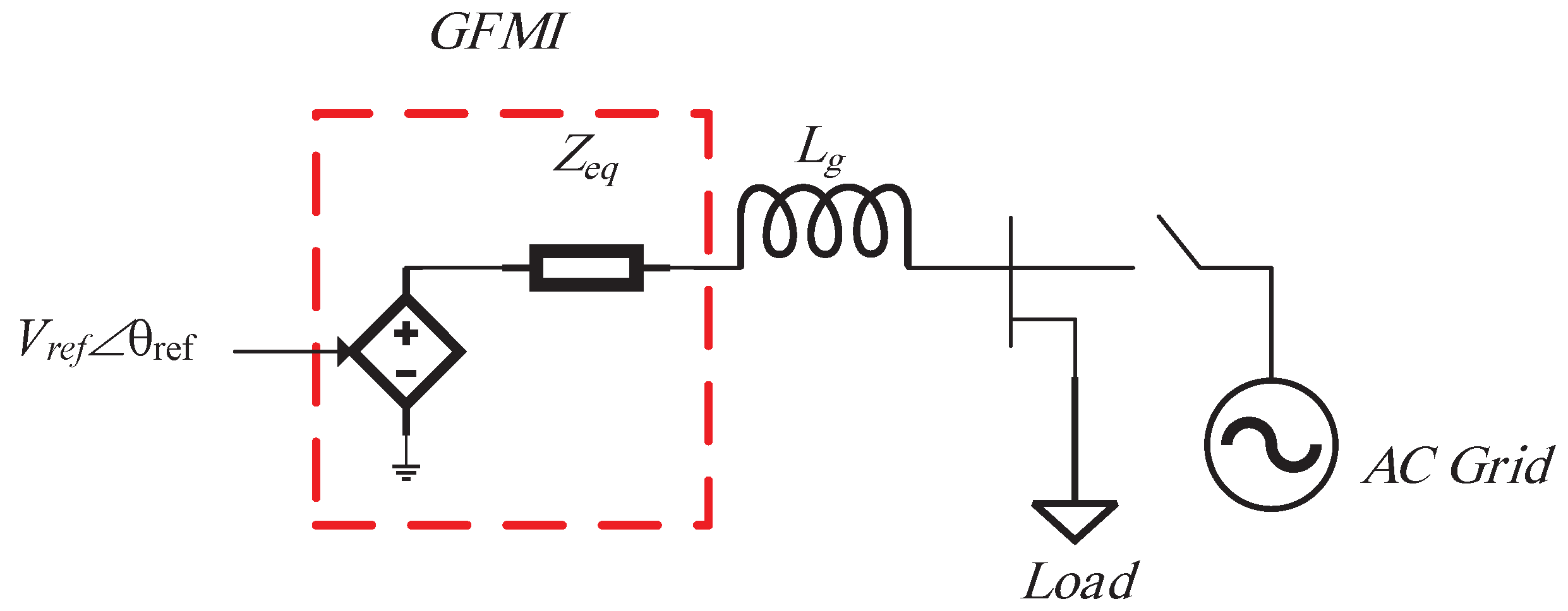
4.2. Transient Stability

The ability of a power system to keep its synchronism in case of large transient disturbances, such as faults, loss of generation or loss of a large load is known as transient stability. Large excursions of bus voltage magnitudes and phase angles, power flows, and other system variables happen when such disturbances interrupt the normal operation of the system. Since large disturbances are the main cause of system transient instability, the nonlinear characteristics of the system are studied for transient stability analysis [79]. Large disturbances result in changes in the rotor angle of the generating units. If these changes are bounded within a certain limit, the generating unit can synchronize with the system and remain stable. Otherwise, the system becomes unstable. To study these changes, the angle dynamics of generating units must be considered, which for an SG, is the swing equation, shown in (15). The swing equation is nonlinear, and numerical methods can be used to determine its solution and to analyze the response of the system to large disturbances in the grid [79].

For GFMIs, the dynamics of the outer control loop set the angle dynamics of the inverter [71]. Therefore, the dynamics of the outer control loop should be studied for the transient stability analysis of GFMIs. Depending on the control scheme, different dynamics and different considerations are taken into account in the transient stability analysis of GFMIs [71]. In the remaining of this section, various methods used for transient stability analysis of GFMIs and a review of existing studies on transient stability of GFMIs are presented.

4.2.1. Methods for Transient Stability Analysis

There are different methods to study transient stability such as numerical methods, Lyapunov’s direct method, and the equal area criterion method (EAC). Each of these methods are discussed in the following sections.

Equal Area Criterion

Neglecting the damping term of (15), the swing equation of an SG is rewritten in (49). Multiplying both sides of (49) by $\frac{2d\delta }{dt}$ and integrating it results in (50). As discussed in Section 4.2, following a disturbance, deviations in phase angle $\delta$ must be bounded to ensure transient stability. Therefore, the integral in (50) must be zero [79]. Thus, the area corresponding to the right-hand side of (42) when $\delta$ is accelerating, known as acceleration area, must be less than or equal to the area corresponding to the right-hand side of (50) when $\delta$ is decelerating, known as deceleration area [79]. Those pairs of $(\delta ,P)$ for which $P_m=P_e$ are called equilibrium points (EPs). If $\frac{d{P}_e}{d\delta }{|}_{{\delta }_{EP}}>0$, the EP is a stable equilibrium point (SEP), and if $\frac{d{P}_e}{d\delta }{|}_{{\delta }_{EP}}<0$, the EP is an unstable equilibrium point (UEP).

$$\frac{d^2\delta }{d{t}^2}=\frac{{\omega }_s}{2H}(P_m-P_e),$$

(49)

$${\left(\frac{d\delta }{dt}\right)}^2=\int \frac{{\omega }_s(P_m-P_e)}{H}d\delta .$$

(50)

Any positive damping in the system improves transient stability of the system. Thus, if the acceleration area of a system with non-negative damping coefficient is less than or equal to its deceleration area, the system is stable. Otherwise, the stability of the system cannot be studied using this method [79]. For GFMIs, $P_m$ and $P_e$ are replaced with $P_{set}$ and P, respectively, [114].

Lyapunov’s Direct Method

Consider the system of (51), where x is an $n\times 1$ vector, $f:D\to R^n$, and $D\subset R^n$, where f is a real $n\times n$ function, and D is a domain in the space of n-dimensional vectors, $R^n$. Lyapunov’s stability theorem states that given that $x=0$ is an EP for (51) and $D\subset R^n$ is a domain containing $x=0$, if there exists a continuously differentiable function $V:D\to R$ such that $V\left(0\right)=0andV\left(x\right)>0$ for $D-\left\{0\right\}$, $x=0$ is a SEP [115]. If $\dot{V}\left(x\right)\le 0inD$, $x=0$ is asymptotically stable, meaning that starting from any initial operating point in D, the system would reach $x=0$ when $t\to \infty$ [115].

$$\dot{x}=f\left(x\right),$$

(51)

where function V with the characteristics mentioned above is called a Lyapunov function or an energy function. Using the outer control loop dynamics of GFMIs as $f\left(x\right)$, this method can be used for transient stability analysis of GFMIs [116].

Numerical or Graphical Methods

Another method to study system transient stability is to numerically solve the angle dynamics equations, or use graphical representations of the system dynamics. This method can be used for systems with complicated angle dynamics and requires no conditions to be met. However, simply deriving the analytical angle dynamics of the system does not provide insight to the system transient stability [117]. Different tools have been used in the literature for graphical study of transient stability. $P-\delta$ and $\dot{\delta }-\delta$ curves are two tools that are mostly used for graphical representations of system dynamics and study of transient stability.

• $P-\delta$ curves: $P-\delta$ curves are used to depict how $\delta$ changes in response to a change in the output active power of generating units [79].
• $\dot{\delta }-\delta$ and $V-\delta$ curves: $\dot{\delta }-\delta$ curves are used to provide a better understanding of how $\delta$ changes when $\dot{\delta }$ changes [117]. $V-\delta$ curves are used to depict how $\delta$ changes with respect to the voltage changes. These curves are usually used when an analytical solution of $\delta$ is difficult to obtain, or the solution does not provide enough insight to the behavior of the system [117]. Based on the dynamics of the system, these curves can be derived either analytically or numerically. Using these curves, the role of different variables and parameters in changes in $\delta$ can be easily shown [117].

4.2.2. Transient Stability of GFMIs

A fault in the grid causes GFMIs to generate large currents. During the fault, to protect the converter switches, current saturation block, shown in Figure 8, sets the reference current of the converter to a predefined value. This results in the GFMI no longer following the reference current set by the voltage control loop and instead injecting a pre-defined reference current into the grid [111]. When studying transient stability of GFMIs, it is assumed that the fault does not trigger the current saturation block, so that the outer control loop remains in charge of setting the inverter current reference [71,118]. Switching of transmission lines, remote faults, or high-impedance faults will not trigger the saturation blocks [118]. Moreover, as transient stability depends on voltage angle dynamics of converters, which are formed by the outer control loop of GFMIs, the inner control loop dynamics are not considered in transient stability studies. This is due to the fast dynamics of inner control loops in comparison with those of the outer control loops [71]. In this section, a review of transient stability analyses of GFMIs for various control schemes is provided.

Droop Control Scheme

Reference [114] proposes adding a saturation block to the active power error in the active power control loop of a droop-controlled grid-connected GFMI to enhance its transient stability. This method results in either increasing the deceleration area or decreasing the acceleration area in $P-\delta$ curve which helps stabilizing the system as the large difference between $P_{ref}$ and P is the cause of transient instability. Reference [119] compares transient stability of a GFLI and a droop-controlled GFMI using their corresponding energy functions. Using energy functions and $\dot{\delta }$-$\delta$ phase portraits, the impact of different factors such as grid impedance, PCC voltage, and control parameters on transient stability of inverters is also studied, and constraints for their stable operation are derived. Reference [120] suggests an asymmetric virtual impedance design in the dq0 frame to improve transient stability of a droop-controlled grid-connected GFMI. The main purpose of this scheme is to provide an SEP for the system in cases it does not exist. The impact of the proposed design on transient stability of GFMIs is investigated using P-$\delta$ curves. Reference [121] compares transient stability of a droop-controlled GFMI and a GFLI by studying a single-converter infinite bus configuration. P-$\delta$ plots and $\dot{\delta }$-$\delta$ curves are used for the transient stability analysis. Using the same tools, the impact of grid strength on transient stability is also studied.

PSC Scheme

In [117], transient stability of a GFMI with the PSC scheme connected to an infinite bus is studied by deriving a complete analytical expression of $\delta$, and using $\dot{\delta }$-$\delta$ curve. It is concluded that as long as there are EPs for the system during disturbances, the system can maintain stability. Furthermore, when there is no EP during disturbances, the maximum phase angle for which clearing the fault results in system stability is analytically calculated.

VSM Control Scheme

In [116], transient stability of a VSM connected to the grid is studied. Using the EAC method and $P-\delta$ curves, it is concluded that by considering the impact of the reactive power control loop of a VSM on its dynamics, the acceleration and deceleration areas become larger and smaller, respectively. This is based on the fact that voltage dynamics affect P, and P affects angle dynamics [116]. This shows the deteriorative impact of the reactive power control loop on transient stability of VSMs. It is suggested to decrease the reference output active power of VSMs during faults to reduce the difference between $P_{ref}$ and P, which is the cause of transient instability. In [116], a Lyapunov function for investigating the transient stability of VSM is introduced, and an algorithm for deriving the critical clearing time (maximum time the protective relay has for its operation until the system becomes unstable), using this Lyapunov function is presented.

Using the EAC method, reference [118] studies transient stability of a VSM connected to the grid. $P-\delta$ curves show that the control error $\mathsf{\Delta }P$ increases when $\delta$ is greater than the power angle of the UEP, which forms a positive feedback mode. This positive feedback mode leads to transient stability issues. Based on this analysis, a mode-adaptive control scheme is presented to make the control error negative during disturbances. In [122], transient stability of a VSM connected to the grid is studied. Using a Lyapunov function, it is shown that a large moment of inertia during disturbances and a small moment of inertia during the recovery time of the system helps improve system transient stability. Thus, [122] proposes an adaptive moment of inertia to improve system transient stability. In [123], to improve transient stability of a VSM GFMI, two voltage boosters are used to change the voltage reference of a GFMI to compensate for the deteriorative impact of the reactive power control loop on transient stability. The main idea behind this scheme is to increase the voltage reference of the VSM during faults to slow down the dynamics of the inverter, which are excited by abrupt changes in the voltage and hence, slow down inverter’s angle dynamics.

By using $\dot{\delta }$-$\delta$ phase portraits and V-$\delta$ curves, [71] shows that droop control without LPFs and PSC control schemes have similar transient response and do not provide virtual inertia although they can continue their stable operation if the system has an EP during a disturbance. Furthermore, [71] shows that droop control with LPFs and VSM control schemes provide inertial response, but can become unstable even if the system has an EP during the disturbance. Transient stability of GFMIs controlled by the droop control and the dVOC methods is studied in [124] using $\dot{\delta }$-$\delta$ curves. The couplings between active and reactive power control loops in the dVOC scheme and their impact on transient stability are also investigated using $\dot{\delta }$-$\delta$ phase portraits and V-$\delta$ curves.

4.2.3. Summary

The existing literature addresses transient stability of GFMIs with different control schemes such as frequency-droop control, PSC, VSM, and dVOC schemes. Using different methods such as EAC, Lyapunov’s direct, and numerical, transient stability of GFMIs is studied and various improvements such as design of an asymmetric virtual impedance for droop-controlled GFMIs [120], introduction of a variable moment of inertia for VSMs [122], and addition of voltage boosters to VSMs [123] are presented. The main focus of most of the studies on transient stability of GFMIs is on providing an SEP for the grid during faults, which is mostly achieved by either decreasing $P_{set}$ or increasing the equivalent impedance between the GFMI and grid. However, there is no study on transient stability of GFMIs in the stand-alone mode. Moreover, transient stability of different configurations, such as parallel connection of GFMIs, and parallel connection of GFMIs with GFLIs are missing in the literature. Also, other control schemes such as matching control and the impact of their control parameters on transient stability of GFMIs are to be addressed in future research.

5. Future Research

In the previous sections, a comprehensive review of GFMI stability studies was presented. This section highlights gaps in the existing literature on the stability of GFMIs for future research. Several studies investigated the small-signal stability of GFMIs with different control schemes and configurations, such as their grid-connected or standalone operation and connection to GFLIs. However, the small-signal stability of GFMIs with different control schemes in an interconnected configuration needs to be studied. Moreover, a study of interactions between the control loops of GFMIs and the control loops of other generating units in the system is imperative. Based on the interaction analysis, new control methods or modifications in the existing control schemes are required to improve overall system stability. As discussed in Section 4.2.2, although the transient stability of GFMIs with droop control, PSC, and VSM control schemes is studied in the literature, studies of transient stability of synchronverter, matching control, and dVOC schemes are missing. Moreover, the impact of interactions of GFMIs with different control schemes in an interconnected system is to be studied in the future. Based on these studies, new methods to improve transient stability of GFMIs are required.

6. Discussion

In contrast to grid-following inverters (GFLIs), grid-forming inverters (GFMIs) can form the voltage magnitude ($V_{ref}$) and angle (${\theta }_{ref}$) at their point of connection to the grid, while supplying active and reactive power to the grid. Hence, GFMIs can operate reliably in the stand-alone mode. Furthermore, since GFMIs do not require a phase-locked loop for synchronization with the grid, they can maintain stability when connected to weak grids. Various schemes are proposed in the existing literature to generate $V_{ref}$ and ${\theta }_{ref}$, such as frequency-droop control, angle-droop control, power synchronization control (PSC), synchronverter control, virtual synchronous machine (VSM) control, virtual oscillator control (VOC), and dispatchable virtual oscillator control (dVOC) schemes of GFMIs. Frequency-droop control, angle-droop control, and PSC schemes generate ${\theta }_{ref}$ using droop curves. The synchronverter scheme emulates the dynamics of synchronous generators (SGs) to generate ${\theta }_{ref}$. The VSM scheme mimics the swing equation of SGs. The matching control scheme uses converter DC-side dynamics to emulate the swing equation of SGs. VOC and dVOC methods use virtual oscillators to provide a constant frequency in the output, with the latter being dispatchable. Except for angle-droop control, VOC, and dVOC schemes, all of these control schemes provide virtual inertia to the system. However, frequency-droop control and PSC schemes do not provide tunable virtual inertia. Synchronverter and VOC schemes do not control the output current of the GFMI and, hence, do not provide overcurrent protection for the converter.

The existing literature delves into the evaluation of small-signal and transient stability aspects in GFMIs under different grid configurations and conditions. These investigations encompass the parallel interconnection of GFMIs, the interfacing of GFMIs with GFLIs, and variations in grid strength. Furthermore, in the existing literature, comparative assessments of small-signal stability and stability margins are conducted across various control methodologies, including frequency droop, PSC, VSM, matching control, and dVOC. An analysis of the impact of control parameters on small-signal stability is carried out through eigenvalue analysis and impedance-based analysis. The provided review of the existing literature concludes that while eigenvalue analysis necessitates a comprehensive model of the system, it surpasses impedance-based analysis due to its capacity to elucidate the system’s small-signal stability through the extraction of participation factors and sensitivity analysis. Within current research, investigations into the transient stability of GFMIs concentrate on achieving system equilibrium during faults. Strategies like asymmetric virtual impedance for droop-controlled GFMIs, varying moment of inertia for VSMs, and rapid voltage enhancement mechanisms are proposed to boost stability. Based on the provided review of this paper, considering the similarities in dynamics between VSMs, synchronverters, and SGs, employing equal area criterion (EAC) method is recommended for analyzing the transient stability of VSMs and synchronverters. In cases involving other control schemes, Lyapunov’s direct method could offer advantages, although the task of identifying a suitable Lyapunov function might pose challenges. The provided review indicates that both numerical and graphical methods can be used for all control schemes, given their independence from specific system conditions. Moreover, graphical methods can provide a better understanding of the transient stability of the system in certain situations.

7. Conclusions

In this paper, two types of inverters used in the power grid, grid-following inverters (GFLIs) and grid-forming inverters (GFMIs), are introduced and compared against each other. The main focus of this paper is the stability of GFMIs. Since the control scheme of GFMIs affects their stability, different GFMI control schemes used in the literature for stability analysis are described. Different categories of power system stability such as rotor angle, frequency, voltage, converter-driven, and resonance are presented, and the small-signal and transient stability studies of GFMIs with different control schemes, as the main two types of GFMI stability studies in the literature, are reviewed. Furthermore, different methods, such as eigenvalue analysis, impedance-based analysis, and robust stability analysis, are used to study the small-signal stability of GFMIs under various operating modes, i.e., stand-alone and grid-connected as well as various configurations such as the parallel connection of GFMIs, and parallel connection of GFMIs and GFLIs are critically reviewed. Moreover, the impacts of different levels of grid strength and load, grid inertia, control loop parameters, transmission line parameters, and grid voltage sags on small-signal stability of GFMIs are discussed. In addition, the studies investigating the impact of different control loops and their control parameters on transient stability of GFMIs in the grid-connected mode using different analysis methods such as equal area criterion (EAC), Lyapunov’s direct method, and numerical and graphical methods are reviewed in this paper. Finally, the existing gaps in the literature regarding the stability of GFMIs are outlined.

References

1. Rathnayake, D.B.; Akrami, M.; Phurailatpam, C.; Me, S.P.; Hadavi, S.; Jayasinghe, G.; Zabihi, S.; Bahrani, B. Grid Forming Inverter Modeling, Control, and Applications. IEEE Access 2021, 9, 114781–114807. [Google Scholar] [CrossRef]
2. Abdel-Rahim, O.; Chub, A.; Vinnikov, D.; Blinov, A. DC Integration of Residential Photovoltaic Systems: A Survey. IEEE Access 2022, 10, 66974–66991. [Google Scholar] [CrossRef]
3. Kroposki, B.; Johnson, B.; Zhang, Y.; Gevorgian, V.; Denholm, P.; Hodge, B.M.; Hannegan, B. Achieving a 100 with Extremely High Levels of Variable Renewable Energy. IEEE Power Energy Mag. 2017, 15, 61–73. [Google Scholar] [CrossRef]
4. Arghir, C.; Jouini, T.; Dörfler, F. Grid-forming control for power converters based on matching of synchronous machines. Automatica 2018, 95, 273–282. [Google Scholar] [CrossRef]
5. Donnini, G.; Carlini, E.; Giannuzzi, G.; Zaottini, R.; Pisani, C.; Chiodo, E.; Lauria, D.; Mottola, F. On the Estimation of Power System Inertia accounting for Renewable Generation Penetration. In Proceedings of the 2020 AEIT International Annual Conference (AEIT), Catania, Italy, 23–25 September 2020; pp. 1–6. [Google Scholar] [CrossRef]
6. Nouti, D.; Ponci, F.; Monti, A. Heterogeneous Inertia Estimation for Power Systems with High Penetration of Converter-Interfaced Generation. Energies 2021, 14, 5047. [Google Scholar] [CrossRef]
7. Milano, F.; Dörfler, F.; Hug, G.; Hill, D.J.; Verbič, G. Foundations and Challenges of Low-Inertia Systems (Invited Paper). In Proceedings of the 2018 Power Systems Computation Conference (PSCC), Dublin, Ireland, 11–15 June 2018; pp. 1–25. [Google Scholar] [CrossRef]
8. Yin, C.; Xie, X.; Xu, S.; Zou, C. Review of oscillations in VSC-HVDC systems caused by control interactions. J. Eng. 2019, 2019, 1204–1207. [Google Scholar] [CrossRef]
9. Li, Y.; Gu, Y.; Green, T.C. Revisiting Grid-Forming and Grid-Following Inverters: A Duality Theory. IEEE Trans. Power Syst. 2022, 37, 4541–4554. [Google Scholar] [CrossRef]
10. Sajadi, A.; Rañola, J.A.; Kenyon, R.W.; Hodge, B.M.; Mather, B. Dynamics and Stability of Power Systems With High Shares of Grid-Following Inverter-Based Resources: A Tutorial. IEEE Access 2023, 11, 29591–29613. [Google Scholar] [CrossRef]
11. Yuefeng, Y.; Jie, Y.; Zhiyuan, H.; Haitian, W. Research on control and protection system for Shanghai Nanhui MMC VSC-HVDC demonstration project. In Proceedings of the 10th IET International Conference on AC and DC Power Transmission (ACDC 2012), Birmingham, UK, 4–5 December 2012; pp. 1–6. [Google Scholar] [CrossRef]
12. Guo, X.; Deng, M.; Wang, K. Characteristics and performance of Xiamen VSC-HVDC transmission demonstration project. In Proceedings of the 2016 IEEE International Conference on High Voltage Engineering and Application (ICHVE), Chengdu, China, 19–22 September 2016; pp. 1–4. [Google Scholar] [CrossRef]
13. Bodin, A. HVDC Light®—A preferable power transmission system for renewable energies. In Proceedings of the 2011 3rd International Youth Conference on Energetics (IYCE), Leiria, Portugal, 7–9 July 2011; pp. 1–4. [Google Scholar]
14. Saad, H.; Fillion, Y.; Deschanvres, S.; Vernay, Y.; Dennetière, S. On Resonances and Harmonics in HVDC-MMC Station Connected to AC Grid. IEEE Trans. Power Deliv. 2017, 32, 1565–1573. [Google Scholar] [CrossRef]
15. Wen, B.; Boroyevich, D.; Burgos, R.; Mattavelli, P.; Shen, Z. Analysis of D-Q Small-Signal Impedance of Grid-Tied Inverters. IEEE Trans. Power Electron. 2016, 31, 675–687. [Google Scholar] [CrossRef]
16. Dong, D.; Wen, B.; Boroyevich, D.; Mattavelli, P.; Xue, Y. Analysis of Phase-Locked Loop Low-Frequency Stability in Three-Phase Grid-Connected Power Converters Considering Impedance Interactions. IEEE Trans. Ind. Electron. 2015, 62, 310–321. [Google Scholar] [CrossRef]
17. Ding, L.; Du, Y.; Lu, X.; Dong, S.; Hoke, A.; Tan, J. Small-Signal Stability Support From Dynamically Configurable Grid-Forming/Following Inverters for Distribution Systems. In Proceedings of the 2022 IEEE Energy Conversion Congress and Exposition (ECCE), Detroit, MI, USA, 9–13 October 2022; pp. 1–7. [Google Scholar] [CrossRef]
18. Huang, L.; Wu, C.; Zhou, D.; Blaabjerg, F. Impact of Virtual Admittance on Small-Signal Stability of Grid-Forming Inverters. In Proceedings of the 2021 6th IEEE Workshop on the Electronic Grid (eGRID), New Orleans, LA, USA, 8–10 November 2021; pp. 1–8. [Google Scholar] [CrossRef]
19. Ding, L.; Lu, X.; Tan, J. Comparative Small-Signal Stability Analysis of Grid-Forming and Grid-Following Inverters in Low-Inertia Power Systems. In Proceedings of the IECON 2021—47th Annual Conference of the IEEE Industrial Electronics Society, Toronto, ON, Canada, 13–16 October 2021; pp. 1–6. [Google Scholar] [CrossRef]
20. Musca, R.; Vasile, A.; Zizzo, G. Grid-forming converters. A critical review of pilot projects and demonstrators. Renew. Sustain. Energy Rev. 2022, 165, 112551. [Google Scholar] [CrossRef]
21. Koller, M.; González Vayá, M.; Chacko, A.; Borsche, T.; Ulbig, A. Primary control reserves provision with battery energy storage systems in the largest European ancillary services cooperation. In Set of Papers, CIGRE Session 46: 21–26 August 2016, Paris, France; ETH: Zurich, Switzerland, 2016; p. 361. [Google Scholar]
22. Mcgregor-Lowndes, M.; Hannah, F. ACPNS Legal Case Notes Series: 2023-87; Matthews v Ausnet Electricity Services Pty Ltd. & Ors; Rowe v Ausnet Electricity Services Pty Ltd. & Ors (Final Ruling): Melbourne, Australia, 2023; Available online: https://eprints.qut.edu.au/241169/ (accessed on 24 June 2024).
23. Manty, A.; Marz, M.; Copp, K.; Sankar, S.; Rector, J.; Fairly, P.; Irwin, G.D. ATC’s Mackinac Back-to-Back HVDC Project: Planning and Operation Considerations for Michigan’s Eastern Upper and Northern Lower Peninsulas; CIGRE USNC-2013 Grid of the Future Symposium, ISO New England Inc.: Holyoke, MA, USA, 2013. [Google Scholar]
24. Marz, M.; Dickmander, D.; Johansson, F.; Irwin, G.; Sankar, S.; Copp, K.; Danielsson, J.; Holmberg, P.; B&v, E.; Manty, A.; et al. Mackinac HVDC Converter Automatic Runback Utilizing Locally Measured Quantities. In Proceedings of the CIGRE Conference, Toronto, ON, Canada, 22–24 September 2014. [Google Scholar]
25. Reserve-Year, H.P. Hornsdale Power Reserve-Year 1 Technical and Market Impact Case Study. Available online: https://www.aurecongroup.com/-/media/files/downloads-library/thought-leadership/aurecon-hornsdale-power-reserve-impact-study-2018.pdf (accessed on 20 April 2024).
26. Gleeson, P. Hornsdale Power Reserve Year 2 Report–Technical and Market Impact Case Study; Aurecon: Sydney, Australia, 2020. [Google Scholar]
27. Tuckey, A.; Round, S. Practical application of a complete virtual synchronous generator control method for microgrid and grid-edge applications. In Proceedings of the 2018 IEEE 19th Workshop on Control and Modeling for Power Electronics (COMPEL), Padua, Italy, 25–28 June 2018; pp. 1–6. [Google Scholar] [CrossRef]
28. Schömann, O.; Sadri, H.; Krüger, W.; Bülo, T.; Hardt, C.; Hesse, R.; Falk, A.; Stankat, P.R. Experiences with Large Grid-Forming Inverters on Various Island and Microgrid Projects. In Proceedings of the Hybrid Power Systems Workshop, Crete, Greece, 22–23 May 2019. [Google Scholar]
29. Anttila, S.; Döhler, J.S.; Oliveira, J.G.; Boström, C. Grid Forming Inverters: A Review of the State of the Art of Key Elements for Microgrid Operation. Energies 2022, 15, 5517. [Google Scholar] [CrossRef]
30. Ebinyu, E.; Abdel-Rahim, O.; Mansour, D.E.A.; Shoyama, M.; Abdelkader, S.M. Grid-Forming Control: Advancements towards 100% Inverter-Based Grids—A Review. Energies 2023, 16, 7579. [Google Scholar] [CrossRef]
31. Aragon, D.; Unamuno, E.; Ceballos, S.; Barrena, J. Comparative small-signal evaluation of advanced grid-forming control techniques. Electr. Power Syst. Res. 2022, 211, 108154. [Google Scholar] [CrossRef]
32. Chandorkar, M.; Divan, D.; Adapa, R. Control of parallel connected inverters in standalone AC supply systems. IEEE Trans. Ind. Appl. 1993, 29, 136–143. [Google Scholar] [CrossRef]
33. Majumder, R.; Chaudhuri, B.; Ghosh, A.; Majumder, R.; Ledwich, G.; Zare, F. Improvement of stability and load sharing in an autonomous microgrid using supplementary droop control loop. In Proceedings of the IEEE PES General Meeting, Minneapolis, MN, USA, 25–29 July 2010; p. 1. [Google Scholar] [CrossRef]
34. Yazdani, S.; Ferdowsi, M.; Shamsi, P. Power Synchronization PID Control Method for Grid-Connected Voltage-Source Converters. In Proceedings of the 2020 IEEE Kansas Power and Energy Conference (KPEC), Manhattan, KS, USA, 13–14 July 2020; pp. 1–6. [Google Scholar] [CrossRef]
35. Zhong, Q.C.; Weiss, G. Synchronverters: Inverters That Mimic Synchronous Generators. IEEE Trans. Ind. Electron. 2011, 58, 1259–1267. [Google Scholar] [CrossRef]
36. Guan, M.; Pan, W.; Zhang, J.; Hao, Q.; Cheng, J.; Zheng, X. Synchronous Generator Emulation Control Strategy for Voltage Source Converter (VSC) Stations. IEEE Trans. Power Syst. 2015, 30, 3093–3101. [Google Scholar] [CrossRef]
37. Rokrok, E.; Qoria, T.; Bruyere, A.; Francois, B.; Guillaud, X. Classification and dynamic assessment of droop-based grid-forming control schemes: Application in HVDC systems. Electr. Power Syst. Res. 2020, 189, 106765. [Google Scholar] [CrossRef]
38. Cvetkovic, I.; Boroyevich, D.; Burgos, R.; Li, C.; Mattavelli, P. Modeling and control of grid-connected voltage-source converters emulating isotropic and anisotropic synchronous machines. In Proceedings of the 2015 IEEE 16th Workshop on Control and Modeling for Power Electronics (COMPEL), Vancouver, BC, Canada, 12–15 July 2015; pp. 1–5. [Google Scholar] [CrossRef]
39. Curi, S.; Groß, D.; Dörfler, F. Control of low-inertia power grids: A model reduction approach. In Proceedings of the 2017 IEEE 56th Annual Conference on Decision and Control (CDC), Melbourne, Australia, 12–15 December 2017; pp. 5708–5713. [Google Scholar] [CrossRef]
40. Arghir, C.; Dörfler, F. The Electronic Realization of Synchronous Machines: Model Matching, Angle Tracking, and Energy Shaping Techniques. IEEE Trans. Power Electron. 2020, 35, 4398–4410. [Google Scholar] [CrossRef]
41. Leyba, E.R.M.; Opila, D.F.; Keith Kintzley, C. Three Phase Dead-Zone Oscillator Control Under Unbalanced Load Conditions. In Proceedings of the 2019 IEEE Electric Ship Technologies Symposium (ESTS), Washington, DC, USA, 14–16 August 2019; pp. 134–140. [Google Scholar] [CrossRef]
42. Tôrres, L.A.B.; Hespanha, J.P.; Moehlis, J. Power supply synchronization without communication. In Proceedings of the 2012 IEEE Power and Energy Society General Meeting, San Diego, CA, USA, 22–26 July 2012; pp. 1–6. [Google Scholar] [CrossRef]
43. Zhang, W.; Cantarellas, A.M.; Rocabert, J.; Luna, A.; Rodriguez, P. Synchronous Power Controller With Flexible Droop Characteristics for Renewable Power Generation Systems. IEEE Trans. Sustain. Energy 2016, 7, 1572–1582. [Google Scholar] [CrossRef]
44. Meng, X.; Liu, J.; Liu, Z. A Generalized Droop Control for Grid-Supporting Inverter Based on Comparison Between Traditional Droop Control and Virtual Synchronous Generator Control. IEEE Trans. Power Electron. 2019, 34, 5416–5438. [Google Scholar] [CrossRef]
45. Awal, M.; Husain, I. Unified virtual oscillator control for grid-forming and grid-following converters. IEEE J. Emerg. Sel. Top. Power Electron. 2020, 9, 4573–4586. [Google Scholar] [CrossRef]
46. Kammer, C.; Karimi, A. Decentralized and Distributed Transient Control for Microgrids. IEEE Trans. Control. Syst. Technol. 2019, 27, 311–322. [Google Scholar] [CrossRef]
47. Madani, S.S.; Kammer, C.; Karimi, A. Data-Driven Distributed Combined Primary and Secondary Control in Microgrids. IEEE Trans. Control. Syst. Technol. 2021, 29, 1340–1347. [Google Scholar] [CrossRef]
48. Jiang, Y.; Bernstein, A.; Vorobev, P.; Mallada, E. Grid-Forming Frequency Shaping Control for Low-Inertia Power Systems. IEEE Control. Syst. Lett. 2021, 5, 1988–1993. [Google Scholar] [CrossRef]
49. Du, W.; Tuffner, F.K.; Schneider, K.P.; Lasseter, R.H.; Xie, J.; Chen, Z.; Bhattarai, B. Modeling of Grid-Forming and Grid-Following Inverters for Dynamic Simulation of Large-Scale Distribution Systems. IEEE Trans. Power Deliv. 2021, 36, 2035–2045. [Google Scholar] [CrossRef]
50. Golestan, S.; Monfared, M.; Freijedo, F.D.; Guerrero, J.M. Performance Improvement of a Prefiltered Synchronous-Reference-Frame PLL by Using a PID-Type Loop Filter. IEEE Trans. Ind. Electron. 2014, 61, 3469–3479. [Google Scholar] [CrossRef]
51. Karimi-Ghartema, M. IEEE Press Series on Microelectronic Systems. In Enhanced Phase-Locked Loop Structures for Power and Energy Applications; IEEE: Piscataway, NJ, USA, 2014; p. 204. [Google Scholar] [CrossRef]
52. Castilla, M.; Vicuna, L.; Miret, J. Control of Power Converters in AC Microgrids; Springer: Berlin/Heidelberg, Germany, 2019; pp. 139–170. [Google Scholar] [CrossRef]
53. Li, S.; Fu, X.; Ramezani, M.; Sun, Y.; Won, H. A novel direct-current vector control technique for single-phase inverter with L, LC and LCL filters. Electr. Power Syst. Res. 2015, 125, 235–244. [Google Scholar] [CrossRef]
54. Yazdani, A.; Iravani, R. Controlled-Frequency VSC System. In Voltage-Sourced Converters in Power Systems: Modeling, Control, and Applications; John Wiley & Sons: Hoboken, NJ, USA, 2010; pp. 245–269. [Google Scholar] [CrossRef]
55. Qoria, T.; Gruson, F.; Colas, F.; Kestelyn, X.; Guillaud, X. Current limiting algorithms and transient stability analysis of grid-forming VSCs. Electr. Power Syst. Res. 2020, 189, 106726. [Google Scholar] [CrossRef]
56. Fan, B.; Liu, T.; Zhao, F.; Wu, H.; Wang, X. A Review of Current-Limiting Control of Grid-Forming Inverters Under Symmetrical Disturbances. IEEE Open J. Power Electron. 2022, 3, 955–969. [Google Scholar] [CrossRef]
57. Qoria, T.; Gruson, F.; Colas, F.; Guillaud, X.; Debry, M.S.; Prevost, T. Tuning of Cascaded Controllers for Robust Grid-Forming Voltage Source Converter. In Proceedings of the 2018 Power Systems Computation Conference (PSCC), Dublin, Ireland, 11–15 June 2018; pp. 1–7. [Google Scholar] [CrossRef]
58. D’Arco, S.; Suul, J.A.; Fosso, O.B. Automatic Tuning of Cascaded Controllers for Power Converters Using Eigenvalue Parametric Sensitivities. IEEE Trans. Ind. Appl. 2015, 51, 1743–1753. [Google Scholar] [CrossRef]
59. Du, W.; Chen, Z.; Schneider, K.P.; Lasseter, R.H.; Pushpak Nandanoori, S.; Tuffner, F.K.; Kundu, S. A Comparative Study of Two Widely Used Grid-Forming Droop Controls on Microgrid Small-Signal Stability. IEEE J. Emerg. Sel. Top. Power Electron. 2020, 8, 963–975. [Google Scholar] [CrossRef]
60. Salha, F.; Colas, F.; Guillaud, X. Virtual resistance principle for the overcurrent protection of PWM voltage source inverter. In Proceedings of the 2010 IEEE PES Innovative Smart Grid Technologies Conference Europe (ISGT Europe), Gothenburg, Sweden, 11–13 October 2010; pp. 1–6. [Google Scholar] [CrossRef]
61. Wang, X.; Blaabjerg, F.; Chen, Z. Autonomous Control of Inverter-Interfaced Distributed Generation Units for Harmonic Current Filtering and Resonance Damping in an Islanded Microgrid. IEEE Trans. Ind. Appl. 2014, 50, 452–461. [Google Scholar] [CrossRef]
62. Cheng, P.T.; Chen, C.A.; Lee, T.L.; Kuo, S.Y. A Cooperative Imbalance Compensation Method for Distributed-Generation Interface Converters. IEEE Trans. Ind. Appl. 2009, 45, 805–815. [Google Scholar] [CrossRef]
63. Rowe, C.N.; Summers, T.J.; Betz, R.E.; Moore, T.G.; Townsend, C.D. Implementing the virtual output impedance concept in a three phase system utilising cascaded PI controllers in the dq rotating reference frame for microgrid inverter control. In Proceedings of the 2013 15th European Conference on Power Electronics and Applications (EPE), Lille, France, 2–6 September 2013; pp. 1–10. [Google Scholar] [CrossRef]
64. Wang, X.; Li, Y.W.; Blaabjerg, F.; Loh, P.C. Virtual-Impedance-Based Control for Voltage-Source and Current-Source Converters. IEEE Trans. Power Electron. 2015, 30, 7019–7037. [Google Scholar] [CrossRef]
65. Kong, L.; Xue, Y.; Qiao, L.; Wang, F.F. Angle Droop Design for Grid-Forming Inverters Considering Impacts of Virtual Impedance Control. In Proceedings of the 2021 IEEE Energy Conversion Congress and Exposition (ECCE), Vancouver, BC, Canada, 10–14 October 2021; pp. 1006–1013. [Google Scholar] [CrossRef]
66. Paquette, A.D.; Divan, D.M. Virtual impedance current limiting for inverters in microgrids with synchronous generators. In Proceedings of the 2013 IEEE Energy Conversion Congress and Exposition, Denver, CO, USA, 15–19 September 2013; pp. 1039–1046. [Google Scholar] [CrossRef]
67. Rodriguez, P.; Candela, I.; Luna, A. Control of PV generation systems using the synchronous power controller. In Proceedings of the 2013 IEEE Energy Conversion Congress and Exposition, Denver, CO, USA, 15–19 September 2013; pp. 993–998. [Google Scholar] [CrossRef]
68. Glover, J.D. Sarma. Power Systems Analysis and Design; PWS Publishing Co.: Pacific Grove, CA, USA, 1987. [Google Scholar]
69. Tielens, P.; Van Hertem, D. The relevance of inertia in power systems. Renew. Sustain. Energy Rev. 2016, 55, 999–1009. [Google Scholar] [CrossRef]
70. Raza, M.; Prieto-Araujo, E.; Gomis-Bellmunt, O. Small-Signal Stability Analysis of Offshore AC Network Having Multiple VSC-HVDC Systems. IEEE Trans. Power Deliv. 2018, 33, 830–839. [Google Scholar] [CrossRef]
71. Pan, D.; Wang, X.; Liu, F.; Shi, R. Transient Stability of Voltage-Source Converters With Grid-Forming Control: A Design-Oriented Study. IEEE J. Emerg. Sel. Top. Power Electron. 2020, 8, 1019–1033. [Google Scholar] [CrossRef]
72. Shabshab, S.C. Dead Zone Oscillator Control for Communication-Free Synchronization of Paralleled, Three-Phase, Current-Controlled Inverters; US Naval Academy: Philadelphia, PA, USA, 2016. [Google Scholar]
73. Johnson, B.B.; Dhople, S.V.; Hamadeh, A.O.; Krein, P.T. Synchronization of Parallel Single-Phase Inverters With Virtual Oscillator Control. IEEE Trans. Power Electron. 2014, 29, 6124–6138. [Google Scholar] [CrossRef]
74. Dhople, S.V.; Johnson, B.B.; Hamadeh, A.O. Virtual Oscillator Control for voltage source inverters. In Proceedings of the 2013 51st Annual Allerton Conference on Communication, Control, and Computing (Allerton), Monticello, IL, USA, 2–4 October 2013; pp. 1359–1363. [Google Scholar] [CrossRef]
75. Johnson, B.B.; Dhople, S.V.; Hamadeh, A.O.; Krein, P.T. Synchronization of Nonlinear Oscillators in an LTI Electrical Power Network. IEEE Trans. Circuits Syst. I Regul. Pap. 2014, 61, 834–844. [Google Scholar] [CrossRef]
76. Seo, G.S.; Colombino, M.; Subotic, I.; Johnson, B.; Groß, D.; Dörfler, F. Dispatchable Virtual Oscillator Control for Decentralized Inverter-dominated Power Systems: Analysis and Experiments. In Proceedings of the 2019 IEEE Applied Power Electronics Conference and Exposition (APEC), Anaheim, CA, USA, 17–21 March 2019; pp. 561–566. [Google Scholar] [CrossRef]
77. Azizi Aghdam, S.; Agamy, M. Virtual oscillator-based methods for grid-forming inverter control: A review. IET Renew. Power Gener. 2022, 16, 835–855. [Google Scholar] [CrossRef]
78. Tayyebi, A.; Groß, D.; Anta, A.; Kupzog, F.; Dörfler, F. Frequency Stability of Synchronous Machines and Grid-Forming Power Converters. IEEE J. Emerg. Sel. Top. Power Electron. 2020, 8, 1004–1018. [Google Scholar] [CrossRef]
79. Kundur, P.; Balu, N.; Lauby, M. Power System Stability and Control; EPRI Power System Engineering Series; McGraw-Hill: New York, NY, USA, 1994. [Google Scholar]
80. Kundur, P.; Paserba, J.; Ajjarapu, V.; Andersson, G.; Bose, A.; Canizares, C.; Hatziargyriou, N.; Hill, D.; Stankovic, A.; Taylor, C.; et al. Definition and classification of power system stability IEEE/CIGRE joint task force on stability terms and definitions. IEEE Trans. Power Syst. 2004, 19, 1387–1401. [Google Scholar] [CrossRef]
81. Hatziargyriou, N.; Milanovic, J.; Rahmann, C.; Ajjarapu, V.; Canizares, C.; Erlich, I.; Hill, D.; Hiskens, I.; Kamwa, I.; Pal, B.; et al. Definition and Classification of Power System Stability—Revisited & Extended. IEEE Trans. Power Syst. 2021, 36, 3271–3281. [Google Scholar] [CrossRef]
82. Terms, Definitions and Symbols for Subsynchronous Oscillations IEEE Subsynchronous Resonance Working Group of the System Dynamic Performance Subcommittee Power System Engineering Committee. IEEE Power Eng. Rev. 1985, PER-5, 37. [CrossRef]
83. Cai, W.; Ying, G.; Li, W.; Wang, Z. The Analysis of a Generator Shaft Crack Cause by Torsional Vibration due to SSR. J. Phys. Conf. Ser. 2021, 2101, 012022. [Google Scholar] [CrossRef]
84. Reader’s guide to subsynchronous resonance. IEEE Trans. Power Syst. 1992, 7, 150–157. [CrossRef]
85. Pourbeik, P.; Ramey, D.G.; Abi-Samra, N.; Brooks, D.; Gaikwad, A. Vulnerability of Large Steam Turbine Generators to Torsional Interactions During Electrical Grid Disturbances. IEEE Trans. Power Syst. 2007, 22, 1250–1258. [Google Scholar] [CrossRef]
86. Shair, J.; Xie, X.; Wang, L.; Liu, W.; He, J.; Liu, H. Overview of emerging subsynchronous oscillations in practical wind power systems. Renew. Sustain. Energy Rev. 2019, 99, 159–168. [Google Scholar] [CrossRef]
87. Milanovic, J.V.; Adrees, A. Identifying Generators at Risk of SSR in Meshed Compensated AC/DC Power Networks. IEEE Trans. Power Syst. 2013, 28, 4438–4447. [Google Scholar] [CrossRef]
88. Adrees, A.; Milanović, J.V. Methodology for Evaluation of Risk of Subsynchronous Resonance in Meshed Compensated Networks. IEEE Trans. Power Syst. 2014, 29, 815–823. [Google Scholar] [CrossRef]
89. Pourbeik, P.; Koessler, R.; Dickmander, D.; Wong, W. Integration of large wind farms into utility grids (part 2—Performance issues). In Proceedings of the 2003 IEEE Power Engineering Society General Meeting (IEEE Cat. No.03CH37491), Toronto, ON, Canada, 13–17 July 2003; Volume 3, pp. 1520–1525. [Google Scholar] [CrossRef]
90. Leon, A.E.; Solsona, J.A. Sub-Synchronous Interaction Damping Control for DFIG Wind Turbines. IEEE Trans. Power Syst. 2015, 30, 419–428. [Google Scholar] [CrossRef]
91. Adams, J.; Carter, C.; Huang, S.H. ERCOT experience with Sub-synchronous Control Interaction and proposed remediation. In Proceedings of the PES T&D 2012, Orlando, FL, USA, 7–10 May 2012; pp. 1–5. [Google Scholar] [CrossRef]
92. Cheng, Y.; Huang, S.H.; Rose, J.; Pappu, V.A.; Conto, J. ERCOT subsynchronous resonance topology and frequency scan tool development. In Proceedings of the 2016 IEEE Power and Energy Society General Meeting (PESGM), Boston, MA, USA, 17–21 July 2016; pp. 1–5. [Google Scholar] [CrossRef]
93. Narendra, K.; Fedirchuk, D.; Midence, R.; Zhang, N.; Mulawarman, A.; Mysore, P.; Sood, V. New microprocessor based relay to monitor and protect power systems against sub-harmonics. In Proceedings of the 2011 IEEE Electrical Power and Energy Conference, Winnipeg, MB, Canada, 3–5 October 2011; pp. 438–443. [Google Scholar] [CrossRef]
94. Wang, X.; Blaabjerg, F. Harmonic Stability in Power Electronic-Based Power Systems: Concept, Modeling, and Analysis. IEEE Trans. Smart Grid 2019, 10, 2858–2870. [Google Scholar] [CrossRef]
95. Wang, X.; Blaabjerg, F.; Wu, W. Modeling and Analysis of Harmonic Stability in an AC Power-Electronics-Based Power System. IEEE Trans. Power Electron. 2014, 29, 6421–6432. [Google Scholar] [CrossRef]
96. Ebrahimzadeh, E.; Blaabjerg, F.; Wang, X.; Bak, C.L. Harmonic Stability and Resonance Analysis in Large PMSG-Based Wind Power Plants. IEEE Trans. Sustain. Energy 2018, 9, 12–23. [Google Scholar] [CrossRef]
97. Wang, X.; Blaabjerg, F.; Liserre, M.; Chen, Z.; He, J.; Li, Y. An Active Damper for Stabilizing Power-Electronics-Based AC Systems. IEEE Trans. Power Electron. 2014, 29, 3318–3329. [Google Scholar] [CrossRef]
98. Yoon, C.; Bai, H.; Beres, R.N.; Wang, X.; Bak, C.L.; Blaabjerg, F. Harmonic Stability Assessment for Multiparalleled, Grid-Connected Inverters. IEEE Trans. Sustain. Energy 2016, 7, 1388–1397. [Google Scholar] [CrossRef]
99. Ebrahimzadeh, E.; Blaabjerg, F.; Wang, X.; Bak, C.L. Modeling and identification of harmonic instability problems in wind farms. In Proceedings of the 2016 IEEE Energy Conversion Congress and Exposition (ECCE), Milwaukee, WI, USA, 18–22 September 2016; pp. 1–6. [Google Scholar] [CrossRef]
100. Fan, L. Modeling Type-4 Wind in Weak Grids. IEEE Trans. Sustain. Energy 2019, 10, 853–864. [Google Scholar] [CrossRef]
101. Li, Y.; Fan, L.; Miao, Z. Stability Control for Wind in Weak Grids. IEEE Trans. Sustain. Energy 2019, 10, 2094–2103. [Google Scholar] [CrossRef]
102. Zhou, J.Z.; Ding, H.; Fan, S.; Zhang, Y.; Gole, A.M. Impact of Short-Circuit Ratio and Phase-Locked-Loop Parameters on the Small-Signal Behavior of a VSC-HVDC Converter. IEEE Trans. Power Deliv. 2014, 29, 2287–2296. [Google Scholar] [CrossRef]
103. Papangelis, L.; Debry, M.S.; Prevost, T.; Panciatici, P.; Van Cutsem, T. Stability of a Voltage Source Converter Subject to Decrease of Short-Circuit Capacity: A Case Study. In Proceedings of the 2018 Power Systems Computation Conference (PSCC), Dublin, Ireland, 11–15 June 2018; pp. 1–7. [Google Scholar] [CrossRef]
104. Liu, H.; Xie, X.; Zhang, C.; Li, Y.; Liu, H.; Hu, Y. Quantitative SSR Analysis of Series-Compensated DFIG-Based Wind Farms Using Aggregated RLC Circuit Model. IEEE Trans. Power Syst. 2017, 32, 474–483. [Google Scholar] [CrossRef]
105. Zhao, F.; Wang, X.; Zhou, Z.; Harnefors, L.; Svensson, J.R.; Kocewiak, L.; Gryning, M.P.S. A General Integration Method for Small-Signal Stability Analysis of Grid-Forming Converter Connecting to Power System. In Proceedings of the 2020 IEEE 21st Workshop on Control and Modeling for Power Electronics (COMPEL), Aalborg, Denmark, 9–12 November 2020; pp. 1–7. [Google Scholar] [CrossRef]
106. Qi, Y.; Deng, H.; Wang, J.; Tang, Y. Passivity-Based Synchronization Stability Analysis for Power-Electronic-Interfaced Distributed Generations. IEEE Trans. Sustain. Energy 2021, 12, 1141–1150. [Google Scholar] [CrossRef]
107. Rosso, R.; Cassoli, J.; Buticchi, G.; Engelken, S.; Liserre, M. Robust Stability Analysis of LCL Filter Based Synchronverter Under Different Grid Conditions. IEEE Trans. Power Electron. 2019, 34, 5842–5853. [Google Scholar] [CrossRef]
108. Sumsurooah, S.; Odavic, M.; Bozhko, S. μ Approach to Robust Stability Domains in the Space of Parametric Uncertainties for a Power System With Ideal CPL. IEEE Trans. Power Electron. 2018, 33, 833–844. [Google Scholar] [CrossRef]
109. Skogestad, S.; Postlethwaite, I. Multivariable Feedback Control: Analysis and Design; John Wiley & Sons, Inc.: Hoboken, NJ, USA, 2005. [Google Scholar]
110. Bryant, J.S.; McGrath, B.; Meegahapola, L.; Sokolowski, P. Small-Signal Modeling and Stability Analysis of a Droop-Controlled Grid-Forming Inverter. In Proceedings of the 2022 IEEE Power & Energy Society General Meeting (PESGM), Denver, CO, USA, 17–21 July 2022; pp. 1–5. [Google Scholar] [CrossRef]
111. Singh, A.; Debusschere, V.; Hadjsaid, N.; Legrand, X.; Bouzigon, B. Slow-interaction Converter-driven Stability in the Distribution Grid: Small-Signal Stability Analysis with Grid-Following and Grid-Forming Inverters. IEEE Trans. Power Syst. 2023, 39, 4521–4536. [Google Scholar] [CrossRef]
112. Yazdani, S.; Ferdowsi, M.; Davari, M.; Shamsi, P. Advanced Current-Limiting and Power-Sharing Control in a PV-Based Grid-Forming Inverter Under Unbalanced Grid Conditions. IEEE J. Emerg. Sel. Top. Power Electron. 2020, 8, 1084–1096. [Google Scholar] [CrossRef]
113. Henriquez-Auba, R.; Lara, J.D.; Roberts, C.; Callaway, D.S. Grid Forming Inverter Small Signal Stability: Examining Role of Line and Voltage Dynamics. In Proceedings of the IECON 2020 The 46th Annual Conference of the IEEE Industrial Electronics Society, Singapore, 18–21 October 2020; pp. 4063–4068. [Google Scholar] [CrossRef]
114. Luo, C.; Ma, X.; Liu, T.; Wang, X. Controller-Saturation-Based Transient Stability Enhancement for Grid-Forming Inverters. IEEE Trans. Power Electron. 2023, 38, 2646–2657. [Google Scholar] [CrossRef]
115. Khalil, H. Nonlinear Control; Always Learning; Pearson: London, UK, 2014. [Google Scholar]
116. Shuai, Z.; Shen, C.; Liu, X.; Li, Z.; Shen, Z.J. Transient Angle Stability of Virtual Synchronous Generators Using Lyapunov’s Direct Method. IEEE Trans. Smart Grid 2019, 10, 4648–4661. [Google Scholar] [CrossRef]
117. Wu, H.; Wang, X. Design-Oriented Transient Stability Analysis of Grid-Connected Converters With Power Synchronization Control. IEEE Trans. Ind. Electron. 2019, 66, 6473–6482. [Google Scholar] [CrossRef]
118. Wu, H.; Wang, X. A Mode-Adaptive Power-Angle Control Method for Transient Stability Enhancement of Virtual Synchronous Generators. IEEE J. Emerg. Sel. Top. Power Electron. 2020, 8, 1034–1049. [Google Scholar] [CrossRef]
119. Fu, X.; Sun, J.; Huang, M.; Tian, Z.; Yan, H.; Iu, H.H.C.; Hu, P.; Zha, X. Large-Signal Stability of Grid-Forming and Grid-Following Controls in Voltage Source Converter: A Comparative Study. IEEE Trans. Power Electron. 2021, 36, 7832–7840. [Google Scholar] [CrossRef]
120. Jin, Z.; Wang, X. A DQ-Frame Asymmetrical Virtual Impedance Control for Enhancing Transient Stability of Grid-Forming Inverters. IEEE Trans. Power Electron. 2022, 37, 4535–4544. [Google Scholar] [CrossRef]
121. Hadjileonidas, A.; Li, Y.; Green, T.C. Comparative Analysis of Transient Stability of Grid-Forming and Grid-Following Inverters. In Proceedings of the 2022 IEEE International Power Electronics and Application Conference and Exposition (PEAC), Guangzhou, China, 4–7 November 2022; pp. 296–301. [Google Scholar] [CrossRef]
122. Hou, X.; Han, H.; Zhong, C.; Yuan, W.; Yi, M.; Chen, Y. Improvement of transient stability in inverter-based AC microgrid via adaptive virtual inertia. In Proceedings of the 2016 IEEE Energy Conversion Congress and Exposition (ECCE), Milwaukee, WI, USA, 18–22 September 2016; pp. 1–6. [Google Scholar] [CrossRef]
123. Ávila Martínez, R.E.; Renedo, J.; Rouco, L.; Garcia-Cerrada, A.; Sigrist, L.; Qoria, T.; Guillaud, X. Fast Voltage Boosters to Improve Transient Stability of Power Systems With 100. IEEE Trans. Energy Convers. 2022, 37, 2777–2789. [Google Scholar] [CrossRef]
124. Yu, H.; Awal, M.A.; Tu, H.; Husain, I.; Lukic, S. Comparative Transient Stability Assessment of Droop and Dispatchable Virtual Oscillator Controlled Grid-Connected Inverters. IEEE Trans. Power Electron. 2021, 36, 2119–2130. [Google Scholar] [CrossRef]
Figure 1. Model of a GFLI as a controlled current source.
Energies 17 03186 g001
Figure 2. Schematic of a typical GFLI.
Energies 17 03186 g002
Figure 3. The control system of a GFLI.
Energies 17 03186 g003
Figure 4. The simplified block diagram of the inner control loop of a GFLI.
Energies 17 03186 g004
Figure 5. Model of a GFMI as a controlled voltage source.
Energies 17 03186 g005
Figure 6. A simple schematic of a typical GFMI.
Energies 17 03186 g006
Figure 7. The block diagram of a typical voltage-mode controller of a GFMI.
Energies 17 03186 g007
Figure 8. The block diagram of a typical current-mode controller of a GFMI.
Energies 17 03186 g008
Figure 9. The simplified block diagram of the current-mode controller of a GFMI.
Energies 17 03186 g009
Figure 10. The block diagram of a GFMI with virtual impedance.
Energies 17 03186 g010
Figure 11. The block diagram of a GFMI with virtual admittance.
Energies 17 03186 g011
Figure 12. Output active and reactive power of the inverter.
Energies 17 03186 g012
Figure 13. Outer control loop of the frequency-droop control scheme.
Energies 17 03186 g013
Figure 14. Active power control loop of the angle-droop control scheme.
Energies 17 03186 g014
Figure 15. Active power control loop of the PSC scheme.
Energies 17 03186 g015
Figure 16. Outer power control loop of the synchronverter control scheme.
Energies 17 03186 g016
Figure 17. Active power control loop of the VSM control scheme.
Energies 17 03186 g017
Figure 18. Outer power control loop of the matching control scheme.
Energies 17 03186 g018
Figure 19. Dead-zone oscillator circuit.
Energies 17 03186 g019
Figure 20. The dead-zone function.
Energies 17 03186 g020
Figure 21. The schematic of the VOC scheme.
Energies 17 03186 g021
Figure 22. dVOC scheme for a GFMI connected to a fully inductive transmission line.
Energies 17 03186 g022
Figure 23. Classification of power system stability [80].
Energies 17 03186 g023
Figure 24. Classification of power system stability considering the impact of power electronic converters [81].
Energies 17 03186 g024
Figure 25. Classification of GFMIs stability [1].
Energies 17 03186 g025
Figure 26. Thevenin equivalent circuit of a GFMI connected to a grid.
Energies 17 03186 g026
Figure 27. System configuration for robust stability analysis.
Energies 17 03186 g027