Evaluation of Prediction Model for Compressor Performance Using Artificial Neural Network Models and Reduced-Order Models

Abstract

In order to save the time and material costs associated with refrigeration system performance evaluations, a reduced-order model (ROM) using highly accurate numerical analysis results and some experimental values was developed. To solve the shortcomings of these traditional methods in monitoring complex systems, a simplified reduced-order system model was developed. To evaluate the performance of the refrigeration system compressor, the temperature of several points in the system where the compressor actually operates was measured, and the measured values were used as input values for ROM development. A lot of raw data to develop a highly accurate ROM were acquired from a VRF system installed in a building for one year, and in this study, specific operating conditions were selected and used as input values. In this study, the ROM development process can predict the performance of compressors used in air conditioning systems, and the research results on optimizing input data required for ROM generation were observed. The input data are arranged according to the design of experiments (DOE), and the accuracy of ROM according to data arrangement is compared through the experiment results.

1. Introduction

In the compressor of an HVAC system, the refrigerant that enters the inlet port is compressed in the compression chamber and discharged at a certain pressure due to the behavior characteristics of the valve located at the discharge port. Therefore, the amount of refrigerant, which determines the performance of the system, is affected by the valve behavior at the compressor discharge port. In order to predict the behavior of the valve located at the compressor discharge port, a numerical model for refrigerant flow and a valve motion model must be considered simultaneously. At this time, the refrigerant flow at the front and rear ends of the valve is affected by the compression process in the compression chamber. The refrigerant flow at the front and rear of the valve can be analyzed with lumped parameter models and computational fluid dynamics models [1,2,3,4,5,6,7,8,9,10,11,12,13,14,15].

Costaglioa et al. [1] proposed a valve dynamic model. The three-dimensional behavior of the valve was expressed as a one-dimensional spring–mass system, and the fluid flow was assumed to be a quasi-static orifice flow. In order to make the three-dimensional behavior of the valve one-dimensional, the area in the valve through which the fluid passes was defined as the effective area. Touber et al. [2] and Ferreira et al. [3] calculated the effective area of the valve through experiments and quantified the complex flow. Lang et al. [4] presented a simplified 1- model for valve behavior using a constant flow area. It provided reliable results and was calculated much faster than CFD numerical models. Hu et al. [5] and Lohn et al. [6] used similar models based on the same equation with some modifications. R. Damle et al. [7] presented an object-oriented 1D numerical simulation of an HVAC system compressor. After modularizing the components of the compressor and generating a numerical analysis model connecting each module with equations, the performance was predicted under two operating conditions for two refrigerants (R600a and R134a) and compared with the experimental results. With the development of methods for studying the interaction between fluids and structures and related numerical analysis techniques, as well as significant improvements in computing power, El Bouzidi et al. [8], and Keramat et al. [9] applied the FSI (Fluid–Structure Interaction) method to a compressor analysis by considering the movement of the valve considering the flow occurring in the micro gap between the valve and the valve lift. Hwang et al. [10] and Park et al. [11] expressed the movement of the valve in the compressor discharge port using the FSI method and verified it through comparison with experimental results. Zhao et al. [12] developed a CFD technique by 3D modeling the compressor. Through this, the relationship between valve movement and pressure pulsation was established. Liu et al. [13] implemented the valve’s vibration and delay movement as an FSI model and developed an empirical equation using the compressor rotation speed as a parameter. Tao et al. [14] implemented the behavior of the compressor discharge valve by developing a 3D FSI model. Aykut Bacak et al. [15] implemented the movement of the compressor discharge valve using the 3D FSI technique and compared the predicted results for three operating conditions with the experimental results.

As mentioned above, performance analysis methods for reciprocating compressors can be divided into one-dimensional and three-dimensional analyses. A one-dimensional analysis requires less time but has low accuracy. Conversely, a three-dimensional analysis can calculate high-accuracy results but requires more time compared to the 1D simulation. Because the advantages and disadvantages of both methods are clear, there is difficulty in selecting an analysis model to evaluate the compressor. To solve these difficulties, a reduced-order model (ROM) has recently been proposed based on highly accurate 3D analysis results. By connecting the ROM generated based on the three-dimensional analysis results with the one-dimensional analysis model, it is possible to compensate for the long analysis time required for the three-dimensional analysis and the low accuracy, which is the drawback of 1D analysis. Reduced-order models are already being applied in various fields [16,17,18,19].

Lucia et al. [16] evaluated the applicability of ROM from a physics perspective. Nayfeh et al. [17] conducted experiments to develop ROM for microbeams and evaluated a theoretical model based on ROM. Yi-dong et al. [18] developed ROM using CFD technology. Through this, the advantages of applying ROM to the optimization of 3D simulation were discussed. Stabile et al. [19] approximated the Navier–Stokes equation through ROM development. And, the stabilization accuracy of the two pressures was compared through POD-Galerkin ROM, applying the finite element method.

For the above studies, ROM has been applied to various fields but has not been used as a method to analyze compressor performance in refrigeration systems. In particular, there were no studies discussing the sampling criteria used for ROM development. In this study, a ROM for predicting the performance of refrigeration system compressors was developed based on a commercial program (ANSYS Workbench 19.0) and experimental results. Additionally, the minimum sample size standard was confirmed through the developed ROM.

2. Modeling

2.1. Response Surface Methodology (RSM)

To establish the standard for the minimum number of samples required to generate a reduced-order model (ROM), the design of experiment (DOE) was studied in this paper. Among the DOE methods, the data count equation used in central composite design (CCD) was investigated. The reason is that the ROM predicts the output parameter using the response surface, and this response surface is generated via the input data according to the CCD. The types of DOE methods are shown in Figure 1. Design of experiment (DOE) is a method of planning experiments to solve a problem. It is designed to obtain the maximum information from the minimum number of experiments. Characteristic value refers to all result values obtained in the form of data from an experiment. Factor refers to an input variable that affects characteristic values. Level means the degree or value of a factor in an experiment and is determined between the maximum and minimum values of the area of interest. For example, in the case of a quantitative factor such as temperature, when the temperature is 100 °C, 150 °C, and 200 °C, the level of the factor called temperature is 3. Design points refer to data consisting of a set of factors and characteristic values [20]. Response surface methodology (RSM) is one of the methods for designing experiments using statistics. RSM can optimize the independent variables and dependent variables. Equation (1) is an equation used to predict the response of the dependent variable by expressing the independent variables as a quadratic equation.

$$Y=a_0+{\sum }_i^k{a}_i{x}_i+{\sum }_i^k{a}_{ii}{x}_i^2+{\sum }_{i=1}^{k-1}{\sum }_{j=i+1}^k{a}_{ij}{x}_i{x}_j+\in$$

(1)

where Y is the experimental response, k is the number of independent variables, a₀ is the constant coefficient, a_i is the linear coefficient, a_ij is the second-order interaction coefficient, a_ii is the quadratic coefficient, and x_i and x_j are the coded values of the independent variables [20,21,22,23,24].

In the case of the response surface design, the central composite design (CCD) method is most used. Figure 2 shows the data batch by CCD. Figure 2a shows the data batch for two factors, x₁ and x₂, and Figure 2b shows the data batch for three factors, x₁, x₂, and x₃. Since the level for each factor is 5, it has five values: −α, −1, 0, +1, and +α. −α is the minimum value of the factor, +α is the maximum value, 0 is the median value, −1 is the value between the minimum value and the median value, and +1 is the value between the maximum value and the median value. The equation for calculating the amount of data required for CCD is shown in Equation (2).

$$N=2^k+2k+n_0$$

(2)

where k refers to the number of factors and refers to the amount of data at the center point. In this study, n₀ was fixed at 1. If there are two factors as shown in Figure 2a, 9 input data must be placed, and if there are three factors as shown in Figure 2b, 15 input data must be placed [22,23,24].

2.2. Data Batch

The input parameters for predicting the performance of a reciprocating compressor are the inlet temperature (T_s), compressor speed (RPS), evaporating temperature (T_e), and condensing temperature (T_c). Using these factors, the cooling capacity, torque, valve stress, and cylinder temperature could be obtained. Since there are four factors, the number of input data required according to Equation (2) is 25.

Table 1. Five-level values for the 4 factors of versions 1 to 4.

	Ts [°C]				RPS [Hz]				Te [°C]				Tc [°C]
ver	1	2	3	4	1	2	3	4	1	2	3	4	1	2	3	4
−α	25	10	10	10	25	10	10	25	−25	−27	−27	−27	35	32	32	32
−1	25	25	10	10	25	25	10	25	−25	−25	−27	−27	35	35	32	32
0	35	32	25	25	50	50	50	50	−22	−22	−22	−22	45	45	45	45
+1	43	35	43	43	70	70	80	80	−20	−20	−17	−17	55	55	58	58
+α	43	43	43	43	70	80	80	80	−20	−17	−17	−17	55	58	58	58

displays four versions of the table, showing five-level values for the four factors. And,

Table 2. The arrangement of input data for 5 levels and 4 factors.

No.	Ts	RPS	Te	Tc	No.	Ts	RPS	Te	Tc
1	0	0	0	0	14	1	−1	1	1
2	+α	0	0	0	15	−1	1	1	1
3	0	+α	0	0	16	1	1	−1	−1
4	0	0	+α	0	17	1	−1	1	−1
5	0	0	0	+α	18	−1	1	1	−1
6	−α	0	0	0	19	1	−1	−1	1
7	0	−α	0	0	20	−1	1	−1	1
8	0	0	−α	0	21	−1	−1	1	1
9	0	0	0	−α	22	1	−1	−1	−1
10	−1	−1	−1	−1	23	−1	1	−1	−1
11	1	1	1	1	24	−1	−1	1	−1
12	1	1	1	−1	25	−1	−1	−1	1
13	1	1	−1	1

shows the arrangement of the input data from 1 to 25 when there are four factors, and the level is five.

Ver1 arranged the data to match the ranges of experimental conditions. The ranges were matched to verify the accuracy of the ROM through experimental results. To check the change in ROM accuracy when the range became wider, Ver2 arranged data over wider ranges than the experimental conditions. To check the change in ROM accuracy when the level is lowered, Ver3 lowered the level from Ver2 from 5 to 3. Ver4 increased the minimum RPS value from 10 to 25 in Ver3. In the case of compressors, accuracy in the low-speed region is most important, so the change in ROM accuracy when the range of the low-speed region changes must be checked.

3. Validation Methods

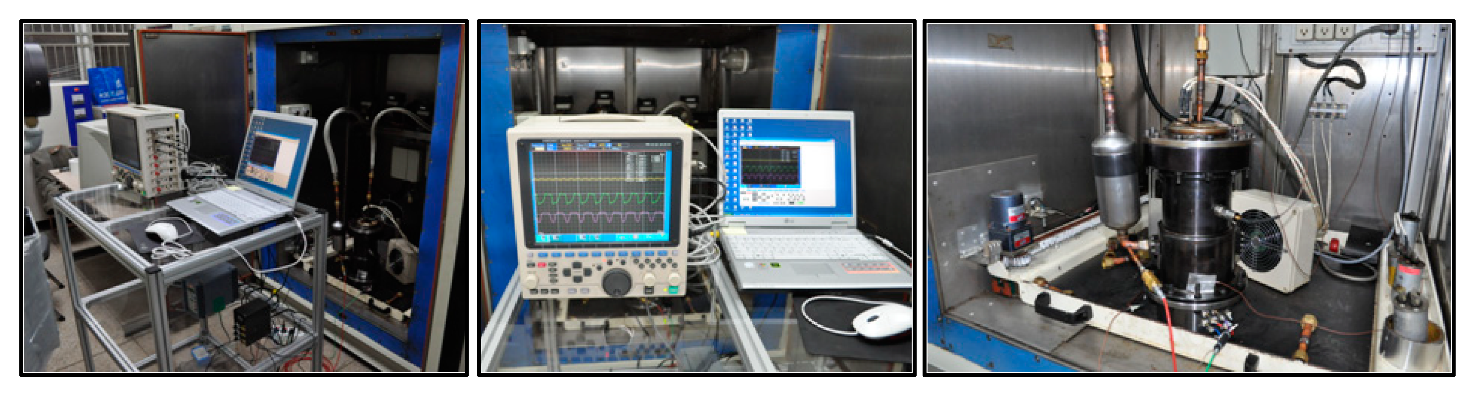
3.1. Experimental Results

To evaluate the ROM accuracy, the thermodynamic properties of the compressor were measured using a calorimeter device as shown in Figure 3. To measure the performance of the compressor, a secondary refrigerant method was used, and experiments were conducted in accordance with “Rated temperature conditions for refrigeration compressors (JIS B8606 [25])” and “Capacity test method for refrigeration compressors (JIS B8600 [26])”. The compressor’s supply power accuracy is ±0.25%, and the temperature and pressure of the inhaled/discharged refrigerant have an accuracy of ±0.3% as shown in

Table 3. The accuracy of ROM as 4 response surface type.

Number of Input Data	191
Response Surface Type	Genetic Aggregation	Non-Parametric Regression	Kriging	Standard Response Surface
ROM accuracy [%]	100	97	93	96
Average error rate [%]	4.3	4.6	5.1	4.4
Max. error rate [%]	9.8	13.0	12.5	11.1
Standard deviation of error rate	2.4	2.8	3.3	2.8

. To evaluate compressor performance, the evaporator temperature and condenser temperature were measured while changing the ambient temperature from 10 to 43 degrees and the rotation speed of the compressor from 10 to 80 Hz. In this study, the standard for ROM accuracy verification was set at 10%. The developed ROM was judged to be reliable if the freezing capacity predicted through the ROM was compared with the experimental value and showed an error below the standard.

At this time, the number of cases showing errors below the standard was defined as ROM accuracy. The number of experimental values for verification was 100 and was expressed as an integer from 0 to 100 to evaluate ROM accuracy. To verify the accuracy of the ROM, the average error rate and maximum error rate were additionally compared.

3.2. Extended ROM

Jeong et al. [27] developed a ROM to predict the refrigeration capacity of a compressor. To develop the ROM, 80 three-dimensional FSI (Fluid–Structure Interaction) data were acquired. To verify the reliability of the training data, the mass flow rate under 7 conditions was compared with the experimental results, and the discharge average temperature under 4 conditions was compared with the experimental results. The error rate of the ROM they developed was less than 10%, and the data generated through the ROM were later used to replace experimental data.

A large amount of data is required to generate a highly accurate ROM, but 3D FSI simulation can only secure a small amount of training data due to its long analysis time.

ROM development requires a lot of raw data. Such data can be obtained using the three-dimensional FSI analysis method and by directly performing experiments on many conditions, but there are significant disadvantages in practical application due to time and material reasons. In this study, the small amount of training data was supplemented by expanding it to a large amount of data using the artificial neural network (ANN) method. And, the expanded ROM data were applied when generating the ROM [28,29].

The ROM was generated by entering training data and expanded data into the ANSYS Workbench 19.0 program. The ANSYS Workbench program provides various response surface types. The prediction accuracy of the ROM varies depending on the response surface type. Response surface types can be divided into four types: Non-Parametric Regression, Genetic Aggregation, Standard Response Surface, and Kriging. Through comparisons with experimental results, the ROM was generated using the response surface type with the highest accuracy [30,31,32].

The ANN model was trained using the training data, and after the training of the ANN model using the training data was completed, new input parameters were entered into the trained ANN model. The trained ANN model predicted the output parameters corresponding to the new input parameters. Through this process, expanded data were obtained. In total, 100 cases of expanded data were generated, and when the 100 expanded data were compared to the experimental results, the reliability of the expanded data was verified because all expanded data had an error rate of less than 10%, as shown in Figure 4. The black squares represent 25 Hz, the red circles represent 30 Hz, the blue triangles represent 50 Hz, and the green triangles represent 70 Hz.

In total, 100 cases of extension data were created through the ANN method, and 100 expanded data were added along with the training data when generating the ROM. The expanded ROM was created based on 191 data, and accuracy verification according to response surface type was conducted through comparison with experimental values.

By including expanded data in the ROM, the average error rate decreased from 4.7% to 4.3% and the highest error rate decreased from 11.8% to 9.8%. And, because the maximum error rate was less than 10%, the ROM accuracy became 100. Figure 5 shows the increase in the ROM accuracy and the decrease in error rate according to the amount of data.

Table 3 shows the accuracy of the ROM as 4 response surface types. The accuracy of ROM was evaluated through four items. Among the four response surfaces, the Genetic Aggregation showed the highest accuracy. The ROM accuracy was 100, the average error rate was 4.3%, the maximum error rate was 9.8%, and the error rate standard deviation was 2.4. The extended ROM, whose accuracy had been verified based on experimental results, was used to verify the response surface and accuracy of the ROM according to the data batch (Ver1, Ver2, Ver3, and Ver4).

4. Results and Discussion

In this study, a ROM was generated in the ANSYS Workbench 19.0. This commercial software program provides a variety of response surface types. In this study, the response surface types of the ROM were fixed to Genetic Aggregation. In

Table 4. Accuracy of ROM by various data batch versions.

	25
Design Point	Ver1	Ver2	Ver3	Ver4
ROM Accuracy [%]	99	97	78	98
Average Error Rate [%]	4.2	3.0	7.2	3.3
Max. Error Rate [%]	10.7	12.	21.9	10.7
Standard deviation of error rate	2.6	2.5	5.1	2.4

, Ver3 recorded the lowest ROM accuracy of 78, and the remaining three versions (Ver1, Ver2, and Ver4) all recorded scores in the low 90s. When comparing the level values for each factor from Table 1, the ROM accuracy decreases when a lot of data with an RPS of 10 Hz are placed.

To check how the response surface was generated in the low-velocity region, the values of T_S, T_e, and T_C were fixed at the intermediate values (25 °C, −22 °C, and 45 °C, respectively), and then two-dimensional response surfaces of cooling capacity according to RPS ware generated. Figure 6 shows the results of comparing the two-dimensional response surfaces of cooling capacity according to RPS. To verify the reliability of the generated two-dimensional response surfaces, the response surface of the extended ROM, verified in the previous section, was used as a reference.

The two-dimensional response surface of Ver1 cannot generate an accurate response surface through extrapolation in the region below 25 Hz and above 70 Hz. The two-dimensional response surface of Ver2 appears to be consistent with the extended ROM in all RPS regions, but the maximum error rate of 56.2% was recorded at 10 Hz. The two-dimensional response surfaces of the extended ROM and Ver3 had a gap between 10 Hz and 45 Hz, with a maximum error rate of 19.7% at 20 Hz. The two-dimensional response surface of the extended ROM and Ver4 had a maximum error rate of 8.7% in the region above 25 Hz, but in the low-speed region below 25 Hz, the two-dimensional response surface of Ver4 could not obtain an accurate response surface through extrapolation. The two-dimensional response surface error rates between the extended ROM and Ver1 to Ver4 are shown in Figure 7.

Ibham et al. [33] explained the limitations of response surface methodology (RSM) in terms of extrapolation and curvature. RSM has the limitation of extrapolation in that it cannot make accurate predictions for areas outside the range of input data. Therefore, to obtain accurate prediction results, predictions must be made only for the area within the range of the input data. Additionally, the response surface is implemented as a second-order polynomial, and if a system has a curvature that does not fit the second-order polynomial of the response surface, the prediction accuracy decreases. In this case, the range of input variables must be reduced to increase the predictive accuracy of the model. For example, if the prediction accuracy is low when data with an RPS of 10 Hz, such as Ver3, are included, the prediction accuracy can be increased by configuring the input data in an area of 25 Hz or higher, excluding 10 Hz data, such as Ver1 and Ver4.

In the case of extrapolation, it was possible to solve the problem by expanding the range of the factor, but in the case of curvature, curvature limitations occurred in different areas depending on the arrangement of the 10 Hz data. The cause of curvature limitations in the mid-to-low-speed range was analyzed through the operating characteristics of the compressor and 3D FSI simulation. Reciprocating compressors have small vibrations due to inertia when operated at high speeds, but when operated at low speeds, large vibrations occur and pulsations in speed and torque occur. And, in the 3D FSI simulation used in this study, changes in compressor rotation speed were linearly reflected in changes in cooling capacity in the mid-to-high-speed range above 25 Hz, but they were not linearly reflected in the low-speed range below 25 Hz. Therefore, the difference in curvature occurred in the two areas at the boundary of 25 Hz, and the curvature limitation of the response surface occurred in the mid-to-low-speed area depending on the arrangement of the 10 Hz data [34,35].

However, because the prediction model must secure high accuracy in all areas, including the low-speed area between 10 Hz and 25 Hz, the ROM was generated using Ver5 data, which is a combination of Ver3 and Ver4 data. Since the two-dimensional response surface of Ver3 has the maximum error rate in the 25 Hz region, the gap that occurs between 10 Hz and 45 Hz can be reduced by adding Ver4 data with data in the 25 Hz region. Additionally, the limitation of the extrapolation that occurs because the two-dimensional response surface of Ver4 does not have input data below 25 Hz can be eliminated by adding 10 Hz data from Ver3. Since Ver3 and Ver4 have the same 16 out of 25 data points, Ver5 is a ROM created based on a total of 34 input data. Figure 8 shows that the two-dimensional response surface of Ver5 matches the two-dimensional response surface of the extended ROM. Unlike Ver2, the response surface error rate graph of Ver5 shows an error rate of less than 10% even in the 10 Hz range. Additionally,

Table 5. ROM accuracy of Ver5.

Number of input data	34
Design points	Ver5
ROM accuracy	100/100
Average error rate [%]	3.8
Max. error rate [%]	9.8
Standard deviation of error rate	2.2

shows that the ROM accuracy of Ver5 was 100, the average error rate was 3.8%, and the maximum error rate was 9.8%.

To check whether Ver5, the supplemented data arrangement, can be applied in other fields, ROM was generated using 1D simulation results, and the 2D response surface and accuracy were verified. Ver5 (only 1D), shown in Figure 9 as the red dotted line, was a ROM generated using the same 34 input data as the data arrangement of Ver5, but the input data used were only 1D data, not 3D FSI data. In the case of Ver5 (only 1D), there was a difference with the two-dimensional response surface of the extended ROM in the area below 25 Hz, but it was not the limit of the extrapolation but the limit of the curvature. The reason for the curvature limit in the area below 25 Hz can be found in the characteristics of 1D simulation. In the case of 1D simulation, unlike 3D FSI, changes in compressor rotation speed are linearly reflected in changes in cooling capacity even in low-speed areas. Because it differs from the actual compressor operating characteristics, the accuracy is lowered in the low-speed range, resulting in curvature limitations. To solve this limitation of curvature, a data mixing method was used in which only 10 Hz input data were replaced with 3D FSI data. Ver5 (1D+3D), shown in Figure 9 as the blue line, was a ROM generated using 1D data for 25 input data above 25 Hz and 3D FSI data for 9 input data corresponding to 10 Hz. The reason why this data mixing method was able to be used is that both 1D and 3D have high accuracy in the mid-to-high-speed range of 25 Hz or higher, so they can be treated as data sharing the same characteristics, and even if 3D FSI data are used only in the low-speed range of less than 25 Hz, no errors occur. Therefore, in Figure 9, the blue dotted line, the two-dimensional response surface of Ver5 (1D+3D), matches the two-dimensional response surface of the extended ROM in all areas.

5. Conclusions

In this study, a reduced-order model (ROM) was generated to predict the performance of HVAC system compressors, and its accuracy was verified through a comparison with experimental results. Because input data are always insufficient due to long simulation times, studies on the minimum amount of input data required to generate ROM should be conducted. Therefore, the effects of arranging input data on ROM accuracy were analyzed.

(1)

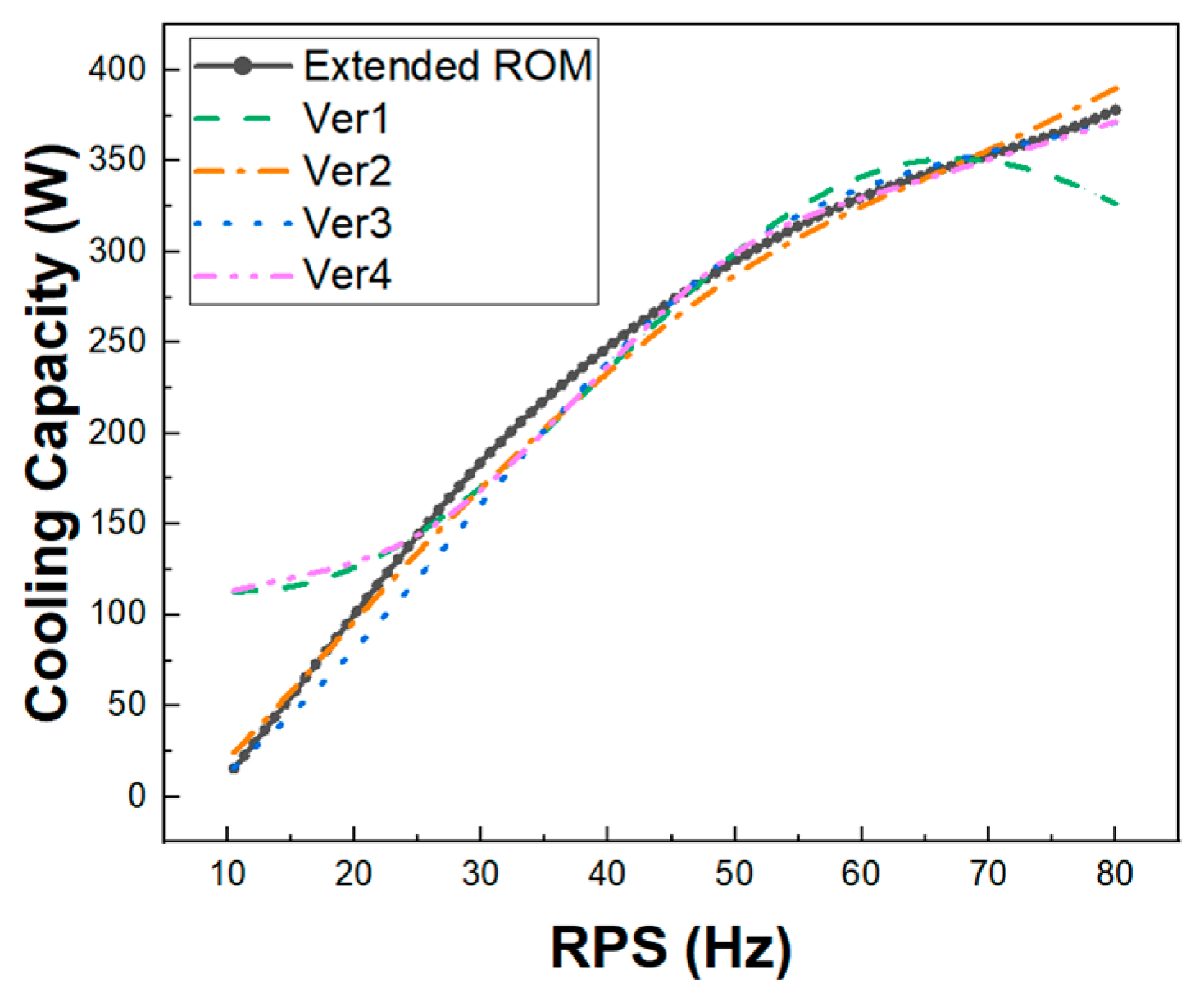
The response surface of the ROM is formed through central composite design (CCD). The data number equation of CCD was used as the standard for the minimum number of input data required to generate the ROM. Since there were four factors and five levels, the minimum number of input data was twenty-five. The ROM was generated according to four versions of data arrangement, with the range of each factor changed.

(2)

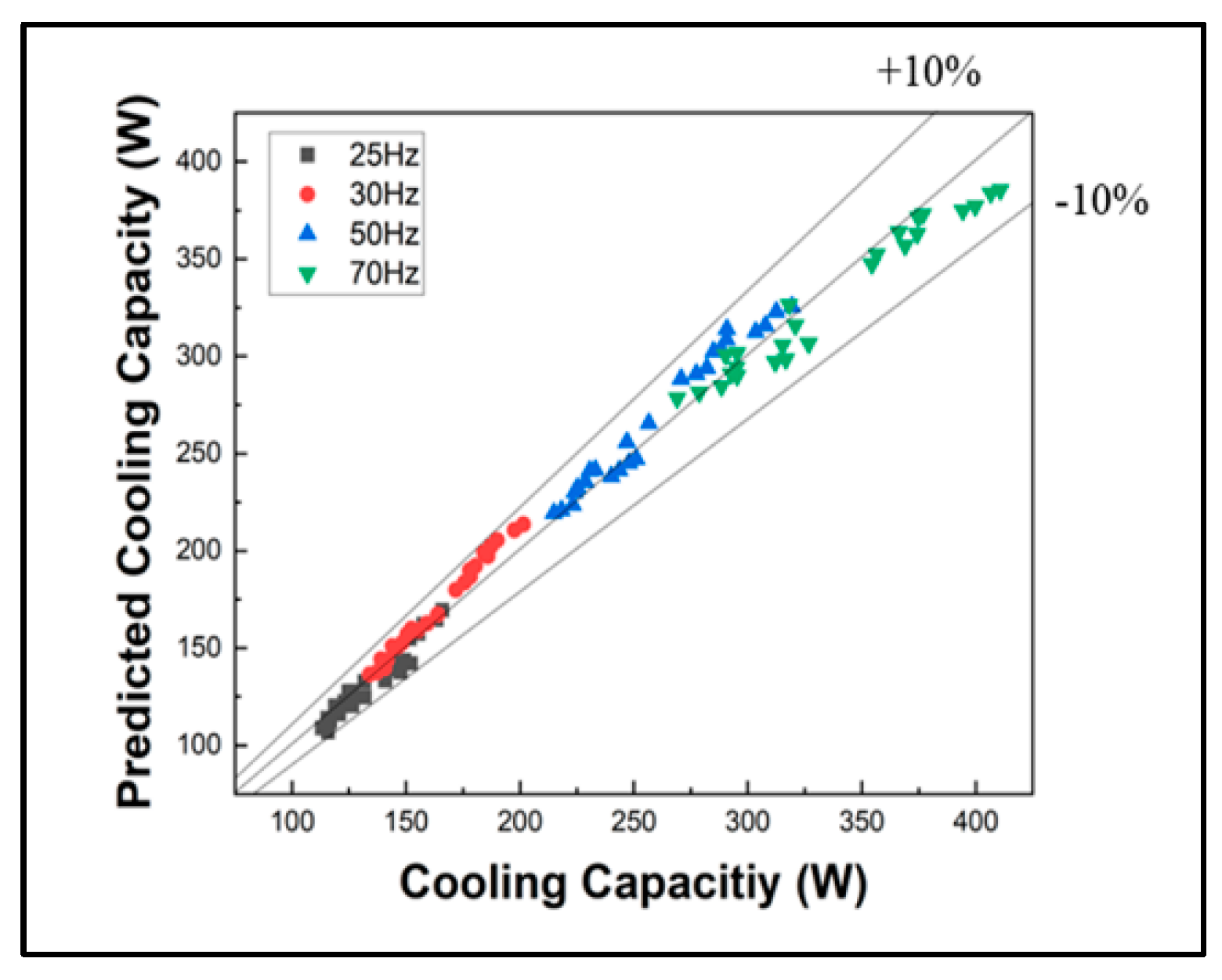
Experimental results and an extended ROM were used to verify the accuracy of the four versions of the ROM. The extended ROM was generated using response surface methodology (RSM) and the artificial neural network (ANN) method. The extended ROM was generated using a total of 191 input data, and its accuracy was verified through experimental results.

(3)

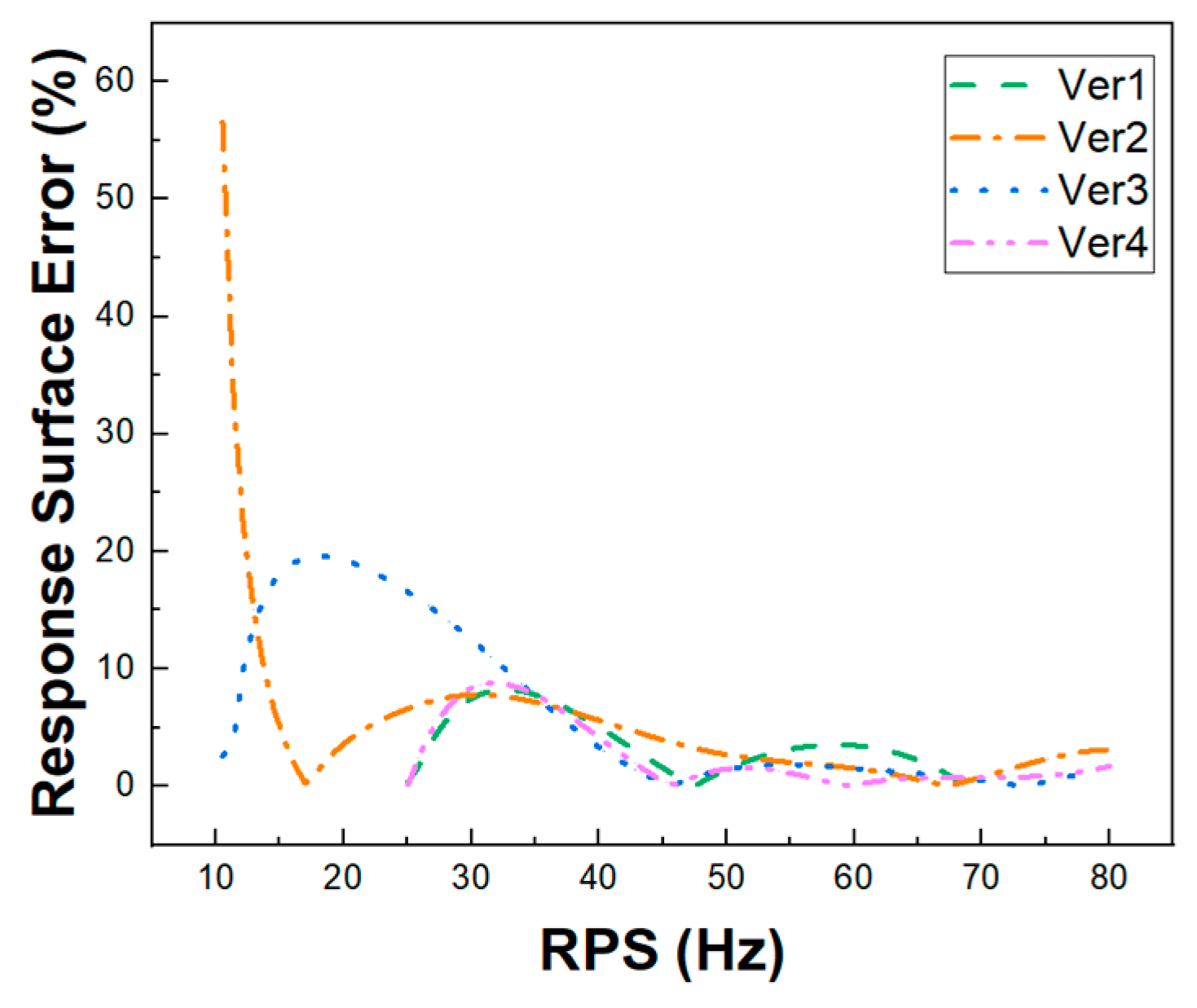
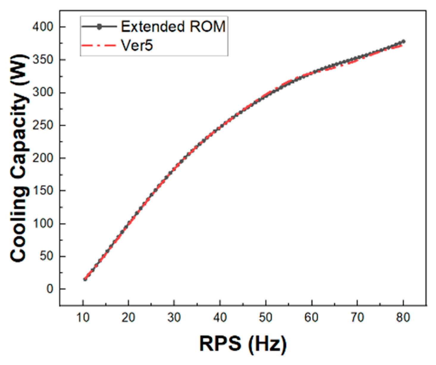
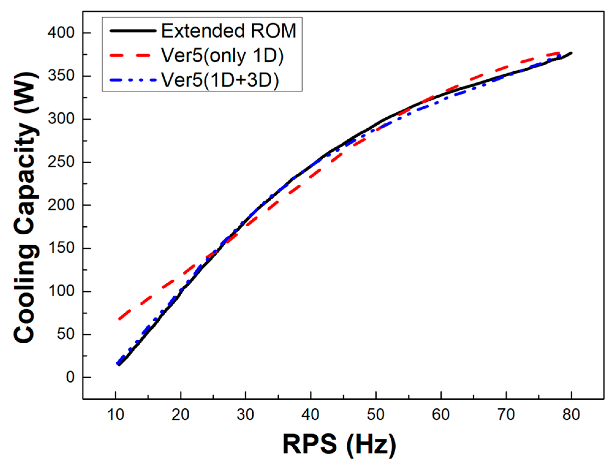
The four versions of the ROM had limitations in the extrapolation and curvature. To compensate for this problem, the data arrangement of Ver5, which was a combination of input data from Ver3 and Ver4, was used to generate the ROM. The ROM accuracy of Ver5 has been verified through experimental results. The ROM accuracy of Ver5 was 100, the average error rate was 3.8%, and the maximum error rate was 9.8%.

References

1. Costagliola, M. The theory of spring-loaded valves for reciprocating compressors. Appl. Mech. 1950, 17, 415–420. [Google Scholar] [CrossRef]
2. Touber, S. A Contribution to the Improvement of Compressor Valve Design. Ph.D. Thesis, Delft University of Technology, Delft, The Netherlands, 1976. [Google Scholar]
3. Ferreira, T.S. Analysis of the Influence of Valve Geometric Parameters on the Effective Flow and Force Areas. In Proceedings of the International Compressor Engineering Conference, West Lafayette, IN, USA, 4–7 August 1986; pp. 558–646. [Google Scholar]
4. Lang, W.; Almbauer, R.; Burgstaller, A.; Nagy, D. Coupling of 0-, 1- and 3-d tool for the simulation of the suction line of a hermetic reciprocating compressor. Int. Comp. Eng 2008, 1272, 1–8. [Google Scholar]
5. Hu, J.; Yang, L.; Shao, L.L.; Zhang, C.L. Generic network modeling of reciprocating compressor. Int. J. Refrig. 2014, 45, 107–119. [Google Scholar] [CrossRef]
6. Lohn, S.K.; Diniz, M.C.; Deschamps, C.J. A thermal model for analysis of hermetic reciprocating compressors under the on-off cycling operating condition. Int. IOP Conf. Ser. Mater. Sci. Eng. 2015, 90, 012068. [Google Scholar] [CrossRef]
7. Damle, R.; Rigola, J.; Pérez-Segarra, C.D.; Castro, J.; Oliva, A. Object-oriented simulation of reciprocating compressors: Numerical verification and experimental comparison. Int. J. Refrig. 2011, 34, 1989–1998. [Google Scholar] [CrossRef]
8. El Bouzidi, S.; Hassan, M.; Ziada, S. Experimental characterization of the self-excited vibrations of spring-loaded valves. J. Fluids Struct. 2018, 76, 558–572. [Google Scholar] [CrossRef]
9. Keramat, A.; Fathi-Moghadam, M.; Zanganeh, R.; Rahmanshahi, M.; Tijsseling, A.S.; Jabbari, E. Experimental investigation of transients-induced fluid–structure interaction in a pipeline with multiple-axial supports. J. Fluids Struct. 2020, 93, 102848. [Google Scholar] [CrossRef]
10. Hwang, I.S.; Park, S.J.; Oh, W.; Lee, Y.L. Linear compressor discharge valve behavior using a rigid body valve model and a FSI valve model. Int. J. Refrig. 2017, 82, 509–519. [Google Scholar] [CrossRef]
11. Park, S.J.; Hwang, I.S.; Oh, W.S.; Lee, Y.L. A study on cycle performance variation of a linear compressor considering valve behavior. J. Mech. Sci. Technol. 2017, 31, 4481–4488. [Google Scholar] [CrossRef]
12. Zhao, B.; Jia, X.; Sun, S.; Wen, J.; Peng, X. FSI model of valve motion and pressure pulsation for investigating thermodynamic process and internal flow inside a reciprocating compressor. Appl. Therm. Eng. 2018, 131, 998–1007. [Google Scholar] [CrossRef]
13. Liu, Z.; Cao, X.; Wang, T.; Jia, W.; Duan, Z. Comparative evaluation of the refrigeration compressor performance under different valve parameters in a trans-critical CO2 cycle. Int. J. Refrig. 2019, 101, 34–46. [Google Scholar] [CrossRef]
14. Tao, W.; Guo, Y.; He, Z.; Peng, X. Investigation on the delayed closure of the suction valve in the refrigerator compressor by FSI modeling. Int. J. Refrig. 2018, 91, 111–121. [Google Scholar] [CrossRef]
15. Bacak, A.; Pınarbaşı, A.; Dalkılıç, A.S. A 3-D FSI simulation for the performance prediction and valve dynamic analysis of a hermetic reciprocating compressor. Int. J. Refrig. 2023, 150, 135–148. [Google Scholar] [CrossRef]
16. Lucia, D.J.; Beran, P.S.; Silva, W.A. Reduced-order modeling: New approaches for computational physic. Prog. Aerosp. Sci. 2004, 40, 51–117. [Google Scholar] [CrossRef]
17. Nayfeh, A.H.; Younis, M.I.; Abdel-Rahman, E.M. Reduced-order models for MEMS applications. Nonlinear Dyn. 2005, 41, 211–236. [Google Scholar] [CrossRef]
18. Lang, Y.-D.; Malacina, A.; Biegler, L.T.; Munteanu, S.; Madsen, J.I.; Zitney, S.E. Reduced order model based on principal component analysis for process simulation and optimization. Energy Fuels 2009, 23, 1695–1706. [Google Scholar] [CrossRef]
19. Stabile, G.; Rozza, G. Finite volume POD-Galerkin stabilized reduced order methods for the parametrized incompressible Navier-Stokes equations. Comput. Fluids 2018, 173, 273–284. [Google Scholar] [CrossRef]
20. Mathews, P.G. Design of Experiments with MINITAB; Quality Press: Milwaukee, WI, USA, 2004. [Google Scholar]
21. Vatanparast, M.; Sarkar, A.; Sahaf, S.A. Optimization of asphalt mixture design using response surface method for stone matrix warm mix asphalt incorporating crumb rubber modified binder. Constr. Build. Mater. 2023, 369, 130401. [Google Scholar] [CrossRef]
22. Suparmaniam, U.; Lam, M.K.; Rawindran, H.; Lim, J.W.; Pa’ee, K.F.; Yong, K.T.L.; Tan, I.S.; Chin, B.L.F.; Show, P.L.; Lee, K.T. Optimizing extraction of antioxidative bio stimulant from waste onion peels for microalgae cultivation via response surface model. Energy Convers. Manag. 2023, 286, 117023. [Google Scholar] [CrossRef]
23. Rastogi, P.M.; Kumar, N.; Sharma, A. Use of response surface methodology approach for development of sustainable Jojoba biodiesel blend with CuO nanoparticles for four stroke diesel engine. Fuel 2023, 339, 127367. [Google Scholar] [CrossRef]
24. Waday, Y.A.; Aklilu, E.G.; Bultum, M.S.; Ancha, V.R. Optimization of soluble phosphate and IAA production using response surface methodology and ANN approach. Heliyon 2022, 8, e12224. [Google Scholar] [CrossRef] [PubMed]
25. JIS B8606; Testing of Refrigerant Compressors. Japanese Standards Association: Tokyo, Japan, 2021.
26. JIS B8600; Standard Condition of Rating Temperature for Refrigerant Compressors. Japanese Standards Association: Tokyo, Japan, 2021.
27. Jeong, H.; Oh, B.; Kim, D.; Lee, K.; Kim, H.; Kim, J.; Choi, G. Development of reduced order model for performance prediction of reciprocating compressor. In 13th International Conference on Compressors and Their Systems; Springer Nature Switzerland: Cham, Switzerland, 2023; pp. 395–407. [Google Scholar]
28. Park, Y.; Choi, M.; Kim, K.; Li, X.; Jung, C.; Na, S.; Choi, G. Prediction of operating characteristics for industrial gas turbine combustor using an optimized artificial neural network. Energy 2020, 213, 118769. [Google Scholar] [CrossRef]
29. Sun, Q.Q.; Zhang, H.C.; Sun, Z.J.; Xia, Y. Ridge regression and artificial neural network to predict the thermodynamic properties of alkali metal Rankine cycles for space nuclear power. Energy Convers. Manag. 2022, 273, 116385. [Google Scholar] [CrossRef]
30. Kim, H.S. Design Techniques for Heat Sink Thermal Analysis Using a Reduced Order Model (ROM). Korean Inst. Power Electron. 2020, 25, 44–49. [Google Scholar]
31. Jin, X.; Zhang, C.; Wang, C. Response surface optimization of machine tool column based on ANSYS workbench. Acad. J. Manuf. Eng. 2020, 18, 162–170. [Google Scholar]
32. Song, B.C.; Bang, I.K.; Han, D.S.; Han, G.J.; Lee, K.H. Structural design of a container crane part-jaw using metamodels. J. Korean Soc. Manuf. Process Eng. 2008, 7, 17–24. [Google Scholar]
33. Veza, I.; Spraggon, M.; Fattah, I.R.; Idris, M. Response surface methodology (RSM) for optimizing engine performance and emissions fueled with biofuel: Review of RSM for sustainability energy transition. Results Eng. 2023, 18, 101213. [Google Scholar] [CrossRef]
34. Im, R.-H.; Yoo, J.-Y.; Lee, K.-W. Method for reducing torque pulsation in reciprocating compressor. In Proceedings of the Korean Electrical Society Conference, Busan, Republic of Korea, 19 July 2010; pp. 21–23. [Google Scholar]
35. Kim, J.-h.; Yang, J.-h.; Ha, J.-i. Design of an extended state observer to improve compressor low-speed operation characteristics. In Proceedings of the Power Electronics Society Conference, Miami, FL, USA, 24–26 September 2023; pp. 252–254. [Google Scholar]
Figure 1. Classification of design of experiments (DOE) methods.
Energies 17 03686 g001
Figure 2. The data batch by central composite design (CCD).
Energies 17 03686 g002
Figure 3. Evaluate equipment of the compressor performance (Calorie-meter).
Energies 17 03686 g003
Figure 4. Reliability of the expanded data predicted using the ANN method.
Energies 17 03686 g004
Figure 5. ROM accuracy according to the amount of data.
Energies 17 03686 g005
Figure 6. Two-dimensional response surfaces of cooling capacity according to RPS.
Energies 17 03686 g006
Figure 7. Two-dimensional response surfaces error rates between the extended ROM and Ver1-4.
Energies 17 03686 g007
Figure 8. Two-dimensional response surfaces of Ver5.
Energies 17 03686 g008
Figure 9. Two-dimensional response surface of Ver5.
Energies 17 03686 g009