1. Introduction
A fuel cell system (FC system) represents a promising alternative to conventional systems due to its potential to mitigate greenhouse gas emissions and reduce reliance on traditional fuels [
1,
2]. However, before such a system can be effectively commercialized, integrated into existing infrastructure, and deployed for practical use, it is essential to thoroughly estimate its technical characteristics. Estimating the performance of an energy system is a pivotal step in its lifecycle, crucial for its successful commercialization, integration into existing infrastructure, and practical utilization. While fuel cell modeling is a common practice, there is often a lack of comprehensive consideration given to the entire system.
This involves a detailed modeling process. Literature reviews have already examined various methodologies for modeling FC operation [
3,
4,
5].
Among these methodologies, several approaches are commonly employed. Numerical models leverage mathematical equations and computational algorithms to simulate the complex physical and chemical processes within the FC system. They offer detailed insights into the system behavior and performance under different operating conditions [
6]. Analytical models aim to represent the FC system’s behavior through mathematical expressions derived from fundamental principles. While less computationally intensive compared to numerical models, they provide valuable insights into system dynamics and performance [
7]. Empirical models are developed based on experimental data and observations. They offer practical insights into system behavior but may lack the theoretical underpinnings of numerical and analytical models [
8]. Data-driven models utilize large datasets to train machine learning algorithms, enabling the system to learn complex patterns and relationships autonomously. With the rise of artificial intelligence and machine learning techniques, data-driven models have gained prominence in FC modeling, offering predictive capabilities and adaptive performance optimization [
9,
10].
Each modeling approach has its strengths and limitations, and the choice of methodology depends on factors such as the complexity of the FC system, available resources, and specific modeling objectives. By employing these diverse modeling techniques, researchers and engineers can gain a comprehensive understanding of FC system behavior, facilitating informed decision-making throughout the system’s lifecycle, from design and optimization to deployment and operation.
For an FC system, it is crucial to thoroughly understand the interaction between the stack and its auxiliary subsystems to develop an FC system with optimal efficiency across its operating range [
11,
12]. In this regard, the digital tool used to design the study/control part of the FC system presented here is derived from [
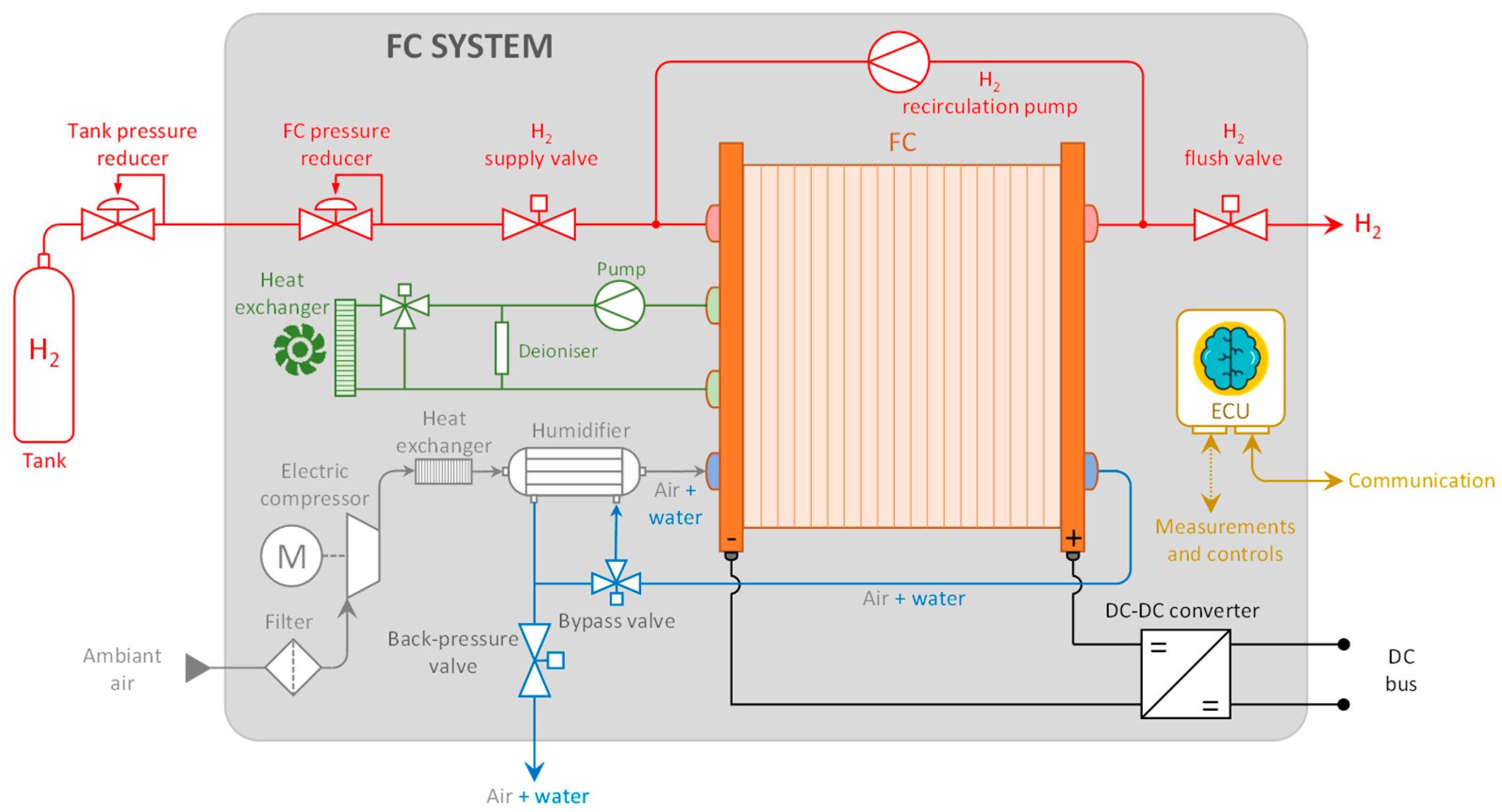
13]. While FC modeling is widespread, the entire system is rarely meticulously considered, especially given computational time constraints [
14]. This involves modeling the entire FC system, as depicted in
Figure 1.
Various components of an FC system can significantly influence its performance and efficiency. Therefore, the decision was made to investigate the operation and efficiency of the main auxiliary components of an FC system: the hydrogen recirculation pump, air compressor, humidifier, and DC/DC converter will be studied accordingly.
2. Modeling
Modeling developed using MATLAB-Simulink provides a precise graphical description of multi-physics couplings and facilitates the easy design of a control scheme. The model is structured around a complex system such as an FC, decomposed into interconnected subsystems, thereby requiring consideration of the principles of physical causality.
2.1. Stack Modeling
The physical behavior of the stack can be divided into several domains. This modeling approach can be characterized as multi-physics, reflecting the coupling of electrochemical, fluidic, and electrical phenomena. The electrochemical aspect involves modeling the redox reactions within the stack, the fluidic part accounts for gas supply and water production, and finally, the electrical part represents the stack’s behavior as a voltage source combined with an impedance.
By integrating these different aspects, the model provides a comprehensive representation of the stack’s behavior, allowing for a deeper understanding of its performance under various operating conditions. The multi-physics approach enables engineers to capture the complex interactions between different physical phenomena within the stack, leading to more accurate predictions and informed design decisions.
2.1.1. Electrochemical Behavior
The electrochemical part revolves around the calculation of a thermodynamic potential
E0. This process involves determining the electrochemical potential of the stack, which plays a critical role in understanding its behavior and performance. In electrochemistry,
E0 typically represents the theoretical redox potential, denoted by the following:
The initial potential is then modified by a change in potential
, leading to the Nernst potential. This step involves adjusting the initial electrochemical potential calculated earlier by incorporating the effect of various factors such as concentration gradients, temperature changes, and other environmental conditions. The resulting Nernst potential reflects the equilibrium potential of the electrochemical reaction within the FC stack, providing crucial insights into its overall performance and behavior. By considering these modifications, the model can more accurately simulate the electrochemical processes occurring within the stack and predict its response to different operating conditions.
The model can account for the temperature-dependent variations in electrochemical reactions within the stack. This approach allows for a more accurate representation of the stack’s electrochemical behavior and facilitates the prediction of its performance under different operating conditions. In the equation below,
Ucell represents the total cell potential in an electrochemical system;
represents the standard cell potential, which is the theoretical voltage of the cell under standard conditions;
accounts for additional electrochemical potentials due to temperature (
T), hydrogen partial pressure (
), and oxygen partial pressure (
), which can influence the overall cell potential; and Δ
E represents any additional factors contributing to the cell potential, such as secondary reactions or ohmic losses. This equation is essential for understanding and predicting the behavior of electrochemical systems, particularly in fuel cells and batteries, where multiple factors influence cell performance.
Similar to the Nernst potential, calculation of the voltage drop ΔE is performed (4). The model computes the voltage drop across the FC stack, taking into account various sources of losses that contribute to the overall decrease in voltage output. These losses include activation losses, which occur due to sluggish reaction kinetics at the electrode surfaces; concentration losses, resulting from mass transport limitations within the electrolyte and electrode materials; and ohmic losses, arising from the resistance encountered by the flow of ions and electrons through the electrolyte and electrodes.
By quantifying these losses, the model can provide valuable insights into the factors influencing the overall efficiency and performance of the FC stack. This information is essential for optimizing the design and operation of the stack to achieve desired performance targets.
This modeling approach involves utilizing the Tafel equation to characterize the activation polarization losses experienced by the FC stack. The Tafel Equation (5) relates the overpotential (difference between the actual electrode potential and the equilibrium potential) to the exchange current density, providing insights into the kinetics of the electrochemical reactions occurring at the electrodes. By incorporating the Tafel law into the model, it becomes possible to accurately simulate the activation losses and their impact on the stack’s performance under various operating conditions, where
A is an empirical coefficient.
Concentration polarization occurs due to the depletion of reactants near the electrode surface, leading to a decrease in reaction rates and voltage losses. Equation (6) represents the mathematical expression used to characterize these concentration losses within the model using an empirical coefficient
B. By incorporating this equation, the model can simulate the concentration polarization effects accurately and assess their impact on the overall performance of the stack under different operating conditions.
Ohmic losses within the FC stack are modeled as the voltage drop across an electrical resistance. This resistance accounts for the electrical resistance encountered by ions as they traverse through the electrolyte and electrodes within the stack. By incorporating this resistance term into the model, it becomes possible to accurately simulate the ohmic losses and their contribution to the overall voltage drop experienced by the stack. This allows for a comprehensive assessment of the stack’s performance and efficiency under different operating conditions.
2.1.2. Fluidic Behavior
The fluidic part comprises the gas circuit located between the hydrogen reservoir, air source, and reaction sites. This section of the model is utilized to calculate the partial pressure used in the electrochemical part. There are two fluidic circuits: one for hydrogen and one for oxygen.
Regarding the air circuit supplying oxygen to the FC, an air compressor is employed. The air compressor will be sized according to the requirement. To model the air compressor, it is initially necessary to determine the mass flow rate of air (8) required for the proper operation of an FC.
where
is the air flow rate (g/s),
is the molar flow rate (mol/s),
M is the molar mass (g/mol),
ν is the stoichiometric ratio (-),
N is the number of cells (-),
is the FC current (A),
F is Faraday’s constant (C), and
is the air nitrogen/oxygen ratio (-).
The hydrogen circuit includes a recirculation pump from the anode outlet to the anode inlet. The mass flow rate of hydrogen is initially calculated using Equation (9).
where
is the hydrogen flow rate (g/s),
is the molar flow rate (mol/s),
M is the molar mass (g/mol),
ν is the stoichiometric ratio (-),
N is the number of cells,
is the FC current (A), and
F is Faraday’s constant (C).
2.1.3. Electrical Behavior
In the electrical section of the model, the focus is on simulating the distribution of charges across the electrodes within the double layer. This phenomenon, known as the double layer effect, significantly influences the electrical behavior of an FC. To accurately represent this effect, a first-order RtCdl circuit is employed, where Rt represents the charge transfer resistance and Cdl denotes the equivalent double layer capacitance.
By incorporating this RtCdl circuit into the model, it becomes possible to simulate the dynamic behavior of the double layer and its impact on the electrical potentials of the FC. This aspect is crucial for understanding how charge distribution affects the overall performance and efficiency of the FC system.
Furthermore, the total voltage output of an FC is determined based on the number of individual cells in the stack (N). This voltage calculation considers the electrical characteristics of each cell and their combined effect on the overall voltage output of the FC system.
All these computations and simulations are performed within a monophysical coupling framework, ensuring that the interactions between different physical phenomena within the FC are accurately represented and integrated into the overall model.
2.2. Auxiliary Components Modeling
Several auxiliary components play crucial roles in an FC system. Among the most influential ones, both in terms of their impact on the FC’s behavior and their economic significance, are the hydrogen recirculation pump, the humidifier, the air compressor, and the DC/DC converter.
2.2.1. Hydrogen Recirculation Pump
Currently, hydrogen recirculation stands out as one of the key aspects of a modern FC system. Recirculation (
Figure 2) involves sending hydrogen back into the anodic circuit with a significant excess. Any unused and humidified hydrogen is reintroduced either using a pump at the circuit’s inlet or through an ejector (passive system). In this context, regular purges are conducted to prevent the accumulation of impurities and water.
Depending on the operating mode, the flow equations are adjusted accordingly in the model. Additionally, the efficiency of the recirculation pump is also accounted for to determine the power consumed by this auxiliary component.
In summary, the hydrogen recirculation loop plays a crucial role in the efficiency, stability, and durability of fuel cells by recovering and reusing unspent hydrogen, while helping to maintain optimal operating conditions for the system.
2.2.2. Humidification
The integration of the humidifier involves estimating the pressure drop based on the air flow rate (Equation (8)). This pressure drop is added to the inlet pressure of the air compressor. For instance, the PermaPure FC-Series moisture exchangers offer unparalleled performance, reliability, and longevity (up to 20,000 h). They provide consistent and reproducible humidification of air and hydrogen within the specified flow range, particularly for automotive applications [
15]. PermaPure moisture exchangers are characterized by low pressure drop and do not require electrical power to operate, which is why we have chosen to consider them in our study. A schematic description of the humidifier’s operation is provided in
Figure 3.
The water production is also calculated in this block using the Equation (10) below:
where
is the mass flow rate of water produced (g/s),
is the molar flow rate (mol/s),
M is the molar mass (g/mol),
N is the number of cells (-),
is the FC current (A), and
F is Faraday’s constant (C).
2.2.3. Air Compressor
It has been reported in the literature that the air compressor can be highly energy-intensive. To model it, it is first necessary to determine the air flow rate (expressed in Equation (8)) required for the proper operation of an FC system.
Subsequently, a performance map of the compressor used is required. In our study, a Rotrex EK10AA compressor is considered [
18]. This compressor offers numerous advantages (high speed of 140,000 rpm, high efficiency, compact and flexible installation, low inertia, and therefore an instant response), making it suitable for the needs of an FC system. The air flow rate of the compressor ranges from 5 to 85 g/s, making it a perfect auxiliary for the studied automotive application. The compressor performance map consists of three elements: air flow rate, pressure ratio, and its efficiency, as shown in
Figure 4.
It is verified that the air flow rate falls within the acceptable limits of the compressor (flow rate above the limit of the pump line). If this is not the case, the air flow rate is adjusted to fall within the limits, and the FC would then operate in excess stoichiometry. Then, based on the air flow rate and pressure ratio, the efficiency of the air compressor is interpolated. Additionally, a final calculation determines the power consumed by the compressor. Note that the data are tailored to the studied system, particularly to the system’s operating power.
2.2.4. DC/DC Converter
The DC/DC converter is a crucial component to consider in an FC system, as it poses a major drawback in terms of lifespan in addition to its cost. Typically, this component has a lifespan of less than 5000 h [
19]. Thus, striking a balance between performance, cost, and lifespan is essential.
One of the most reputable manufacturers in the field is Brusa [
20]. An example of the operating chain of this company is illustrated in
Figure 5. These tools offer numerous advantages such as voltage, current, or power control; regulation of input or output; liquid cooling; and very high efficiency (>95%).
Regarding the modeling, it is inspired by [
21]. Assuming that the time constant of the inductance is much larger than the switching period of the DC/DC converter, its modeling can be defined as follows:
with
where
is the current passing through the inductance,
is the value of the inductance,
is the resistance of the smoothing inductance,
is the output voltage of the converter,
is the chopping modulation ratio of the DC/DC converter,
is the DC bus voltage, and
is the efficiency of the converter.
3. Results and Analysis
To validate the model, several approaches can be taken. First, by comparing the polarization curve predicted by the model with experimental data, we can assess its accuracy in representing the FC’s performance under different operating conditions. This involves varying parameters such as temperature, pressure, and stoichiometry and observing how the model responds in comparison to real-world measurements.
Secondly, dynamic simulations can be conducted using realistic load profiles, such as those from standardized driving cycles such as the WLTP. By simulating the transient response of the FC system to dynamic load changes, we can evaluate its ability to accurately predict the system’s behavior over time. This validation helps ensure that the model captures the system’s dynamic characteristics, including start-up, transient response, and steady-state operation.
Overall, these validation steps provide confidence in the model’s predictive capabilities and its suitability for analyzing the performance of FC systems under various operating conditions and loads.
3.1. Polarization Curve
An optimization algorithm was utilized to adjust the parameters of the Nernst equation based on a reference polarization curve provided by an FC supplier. This adjustment aimed to ensure that the model closely matches the behavior observed in the reference curve. To assess the accuracy of the model, we analyzed the performance of a PowerCell FC, for which the reference polarization curve was supplied by the manufacturer (conc. fuel: 70% H
2 in N
2; T
in coolant: 72 °C; dew point A/C: 46.4/52.4 °C; stoic A/C: 1.5/2.0; pressure A/C: 0.35/0.25 barg). This curve, depicted in
Figure 6, serves as a benchmark for evaluating the model’s fidelity to real-world data.
Once the parameters are determined, it is possible to modify the input parameters of the model such as the electrical load (current or power) and pressures/flows/stoichiometric ratios and observe the model’s response to these modifications.
In this section, experimental results are compared to model predictions. Depending on the input parameters (stoichiometries and pressures), the results are compared, and for this purpose, polarization curves and fluid flows are plotted on the same graphs.
For all experiments, the anode pressure was fixed at 2 bar with a stoichiometric ratio also maintained at 2. The experiments showed that the cathodic stoichiometric ratio and relative humidity had virtually no influence on the polarization curve results, as shown in
Figure 7. Indeed, during this initial behavioral study, the cathode pressure was 1.75 bar, the stoichiometric ratio varied between 2 and 2.5, and the relative humidity varied between 30 and 50%. It can be observed that the results are very similar, with minimal variations on the polarization curves. Regarding the modeling, it can be observed that the predictions are consistent with the experimental measurements.
In
Figure 8, polarization curves are plotted for different cathode pressures ranging from 1.5 to 2.5 bar, with a constant stoichiometry of 2 at the cathode. A decrease in voltage for the same current is observed as the pressure decreases. This observation highlights the significant impact of pressure on the performance of the FC system. Despite the variations in pressure, the model accurately predicted the system behavior, as evidenced by the near overlap of the experimental polarization curves with the curves predicted by the model. This agreement between the experimental results and model predictions demonstrates the reliability and effectiveness of the developed model in studying FC performance under different operating conditions.
While the cathodic variation in stoichiometric ratio (2 and 2.5) had a minor impact on the polarization curve, it notably influenced gas flow rates. The comparison between the experimental and analytical results of air and hydrogen fluxes (
Figure 9) across different stoichiometric ratios (1.5 at the anode/2 or 2.5 at the cathode) revealed that the model effectively predicted the gas flow dynamics necessary for optimal FC operation.
Overall, the model provides a comprehensive understanding of the studied FC’s performance, allowing for precise predictions of its capabilities. This is demonstrated by the close agreement between the experimental measurements and the model predictions when analyzing polarization curves. The detailed comparison between the two sets of data revealed a consistent and reliable correspondence, indicating the model’s effectiveness in capturing the behavior of the FC under different operating conditions. This level of accuracy and consistency underscores the model’s utility as a valuable tool for studying and optimizing FC systems.
3.2. WLTP Cycle
In this section, the focus is on observing the response of the FC system to a demand cycle smoothed according to the Worldwide Harmonized Light Vehicle Test Procedure (WLTP) in order to meet international standards (
Figure 10). In the pursuit of enhancing fuel cell (FC) longevity, a minimal current demand is recommended, steering clear of operations at the open circuit voltage (OCV) and employing a restricted current ramp. This approach is facilitated by the integration of a battery within the powertrain system. By orchestrating a symbiotic interplay between the fuel cell and the battery, a delicate balance is achieved, optimizing the performance while safeguarding the durability of the fuel cell. This strategy not only mitigates the strain on the FC but also ensures sustained and efficient power delivery, thereby prolonging the overall lifespan of the fuel cell system.
To delve deeper into the system operation,
Figure 11 provides a schematic representation illustrating how power is distributed within the system. This schematic highlights the interplay between the reference current, electrical power, and gas flow, emphasizing the role of efficiency considerations for the various auxiliary components. Such a comprehensive view helps elucidate the intricate functioning of the system and its control mechanisms.
Therefore, it is possible to observe various outcomes and explore the capabilities of the FC system. In this section, the most significant results are presented, focusing on power outputs and efficiencies.
The evolution of different power outputs is depicted in
Figure 12, illustrating the theoretical power of hydrogen (Equation (14)), the power generated by the FC system, and the various power consumptions of auxiliary components (air compressor, recirculation pump, and DC/DC converter).
where
is the hydrogen flow rate (g/s) as expressed in Equation (9), and
is the mass-specific energy of hydrogen (J/g).
The theoretical power output over this cycle reaches 100 kW, whereas the FC system’s power output only reaches 45 kW. The most energy-intensive auxiliary component, the air compressor, can consume up to 7 kW.
The following efficiencies were also studied (
Figure 13): the stack efficiency
, the efficiencies of the auxiliary components, and the system efficiency (when the auxiliary components are accounted for). The stack efficiency ranges from 77% (when the current load is minimal) to 46% when the current demand is maximal, i.e., 400 A. Regarding the system, the efficiency is naturally lower than that of the stack. The maximum efficiency is 69% (minimal load), slightly lower than that of the stack at high regime.
Overall, the power response of the FC system to the applied reference current is quite promising. It demonstrates the capability to accommodate high current demands effectively. However, to mitigate dynamic constraints such as fluctuations in current, it is essential to integrate the FC system with a battery. This integration will ensure smoother operation and enhance the overall stability and performance of the system.
3.3. Analysis and Discussion
The model has been validated using polarization curves. The decision to investigate only the cathode in the fuel cell was made for several reasons. The importance of cathodic stoichiometry lies in its significant impact on the overall performance and efficiency of a fuel cell. The oxygen reduction reaction at the cathode is typically the rate-limiting step and is more sensitive to stoichiometric variations compared to the hydrogen oxidation at the anode. This makes the availability of oxygen at the cathode crucial for the fuel cell’s performance. Additionally, the cathodic reaction produces water, necessitating effective water management to prevent flooding or membrane dehydration. Maintaining appropriate humidity levels in the membrane is vital for ionic conductivity and overall performance. High stoichiometric ratios at the cathode also help reduce concentration losses by ensuring a steady supply of oxygen, thereby optimizing the reaction and improving energy efficiency. Furthermore, based on the experience gained through collaboration with various industries (particularly in the automotive field), it has been observed that they conduct studies on variations in cathodic stoichiometry, while anodic stoichiometry is often stable and fixed at 1.5. We thus chose to adhere to this parameter setting in line with current studies.
The model simulates transient responses to variations in load demand, including start-up, shutdown, and load-following capabilities. Control strategies for energy management can be incorporated to ensure stable and efficient operation under dynamic load conditions. The model simulates the dynamics of the hydrogen and oxygen supply, including pressure regulators and flow controllers, to ensure appropriate delivery rates under transient conditions. Simulation of the effects of water production and removal is also taken into account, as water management is essential for maintaining membrane hydration and preventing flooding or drying out. Finally, the model includes auxiliary components such as compressors, humidifiers, and pumps to ensure they meet the dynamic requirements of the FC system.
Concerning the limitations of the model, assumptions about steady-state conditions, uniform temperature, and pressure distribution might not hold true in real-world operations. Temperature and pressure might vary more widely than those modeled. Real control systems may have time delays and inaccuracies that are not fully captured in the simulation. Environmental conditions such as temperature fluctuations, vibrations, and contamination can also affect FC performance but may not be fully accounted for in the model. Over time, components of the FC degrade, affecting the performance in ways that are difficult to predict and model accurately. All the points mentioned previously can influence the results and create a discrepancy with the experimental results. Understanding the ageing process of the FC could therefore offer useful perspectives.
4. Conclusions
In this article, we developed a detailed model of an FC system using MATLAB-Simulink. This model allowed us to analyze the performance and characteristics of the studied FC system accurately. Specifically, we examined the impact of auxiliary components such as the hydrogen recirculation pump, humidifier, air compressor, and DC/DC converter on the overall efficiency of the system.
In the first part, the model was validated using a polarization curve. The difference between the experimental measurements and the theoretical estimation was only 3%. Considering the efficiency of the model, it was interesting to study the transient response possibilities of an FC system. For this, a WLTP cycle was applied. It was found that the air compressor, in particular, consumes a significant amount of energy, underscoring its importance in the design and optimization of FC systems. This in-depth analysis helped us better understand the interactions between the various components of the system and their implications in overall performance.
For future perspectives, several avenues could be explored. For instance, we could seek to identify components that could benefit from optimization to reduce their energy consumption. Additionally, exploring optimal configurations for coupling between the FC and battery, considering the lifespan of each component based on its usage, could offer significant benefits in terms of system efficiency and durability.
Author Contributions
Conceptualization, A.P. and D.B.; methodology, A.P. and D.B.; software, A.P. and P.S.; validation, A.P. and D.B.; formal analysis, A.P.; resources, D.B.; writing—original draft preparation, A.P.; writing—review and editing, A.P., P.S. and D.B.; project administration, D.B.; funding acquisition, D.B. All authors have read and agreed to the published version of the manuscript.
Funding
This research received no external funding.
Data Availability Statement
Data is unavailable due to privacy restrictions.
Acknowledgments
This work was supported by the EIPHI Graduate School (contract ANR-17-EURE-0002) and the Region Bourgogne Franche-Comté.
Conflicts of Interest
The authors declare no conflicts of interest.
References
- Wu, H.W. A review of recent development: Transport and performance modeling of PEM fuel cells. Appl. Energy 2016, 165, 81–106. [Google Scholar] [CrossRef]
- Pahon, E.; Bouquain, D.; Hissel, D.; Rouet, A.; Vaquier, C. Performance analysis of proton exchange membrane fuel cell in automotive applications. J. Power Sources 2021, 510, 230385. [Google Scholar] [CrossRef]
- Wang, C.Y. Fundamental Models for Fuel Cell Engineering. Chem. Rev. 2004, 104, 4727–4766. [Google Scholar] [CrossRef] [PubMed]
- Arif, A.M.; Cheung, S.C.P.; Andrews, J. Different Approaches Used for Modeling and Simulation of Polymer Electrolyte Membrane Fuel Cells: A Review. Energy Fuels 2020, 34, 11897–11915. [Google Scholar] [CrossRef]
- Zhao, J.; Li, X.; Shum, C.; McPhee, J. A Review of physics-based and data-driven models for real-time control of polymer electrolyte membrane fuel cells. Energy AI 2021, 6, 100114. [Google Scholar] [CrossRef]
- Goshtasbi, A.; Pence, B.L.; Ersal, T.T. Computationally efficient pseudo-2D non isothermal modeling of polymer electrolyte membrane fuel cells with two-phase phenomena. J. Electrochem. Soc. 2016, 163, F1412-32. [Google Scholar] [CrossRef]
- Hong, L.; Chen, J.; Liu, Z.; Huang, L.; Wu, Z. A nonlinear control strategy for fuel delivery in PEM fuel cells considering nitrogen permeation. Int. J. Hydrogen Energy 2017, 42, 1565–1576. [Google Scholar] [CrossRef]
- Zhang, X.; Yang, D.; Luo, M.; Dong, Z. Load profile based empirical model for the lifetime prediction of an automotive PEM fuel cell. Int. J. Hydrogen Energy 2017, 42, 11868–11878. [Google Scholar] [CrossRef]
- Khan, S.S.; Shareef, H.; Mutlag, A.H. Dynamic temperature model for proton exchange membrane fuel cell using online variations in load current and ambient temperature. Int. J. Green Energy 2019, 16, 361–370. [Google Scholar] [CrossRef]
- Vichard, L.; Harel, F.; Ravey, A.; Venet, P.; Hissel, D. Degradation prediction of PEM fuel cell based on artificial intelligence. Int. J. Hydrogen Energy 2020, 45, 14953–14963. [Google Scholar] [CrossRef]
- Spiegel, C. PEM Fuel Cell Modeling and Simulation Using MATLAB; Elsevier: Amsterdam, The Netherlands, 2011. [Google Scholar]
- Dicks, A.; Rand, D.A.J. Fuel Cell Systems Explained; Wiley: Hoboken, NJ, USA, 2018. [Google Scholar]
- Boulon, L.; Hissel, D.; Bouscayrol, A.; Péra, M.C. From Modeling to Control of a PEM Fuel Cell Using Energetic Macroscopic Representation. IEEE Trans. Ind. Electron. 2010, 57, 1882–1891. [Google Scholar] [CrossRef]
- Yang, Z.; Du, Q.; Jia, Z.; Yang, C.; Xuan, J.; Jiao, K. A comprehensive proton exchange membrane fuel cell system model integrating various auxiliary subsystems. Appl. Energy 2019, 256, 113959. [Google Scholar] [CrossRef]
- Blunier, B.; Miraoui, A. Piles à Combustible—Principes, Modélisation, Applications avec Exercices et Problèmes Corrigés; Ellipses: Paris, France, 2007. [Google Scholar]
- Han, J.; Feng, J.; Chen, P.; Liu, Y.; Peng, X. A review of key components of hydrogen recirculation subsystem for fuel cell vehicles. Energy Convers. Manag. 2022, 15, 100265. [Google Scholar] [CrossRef]
- PermaPure®. Moisture Control Experts. Available online: https://www.permapure.com/environmental-scientific/products/gas-humidification/fc-series-humidifiers/ (accessed on 23 July 2024).
- Kolstrup, A. Project Rotrex. Rotrex Communication. Development of the Rotrex Supercharger to Compression of Water Vapor. Available online: https://www.oil-club.ru/forum/applications/core/interface/file/attachment.php?id=267233 (accessed on 23 July 2024).
- Wang, H.; Gaillard, A.; Hissel, D. A review of DC/DC converter-based electrochemical impedance spectroscopy for fuel cell electric vehicles. Rev. Bras. Econ. 2019, 141, 124–138. [Google Scholar] [CrossRef]
- BRUSA. Datasheet BDC546—Bidirectional 750 V DC/DC-Converter. The Global Benchmark in High Power FC Applications. Available online: https://www.brusahypower.com/wp-content/uploads/2021/03/BRUSA_Factsheet_BDC546.pdf (accessed on 23 July 2024).
- Fernandez, A.M.; Kandidayeni, M.; Boulon, L.; Chaoui, H. An adaptive state machine based energy management strategy for a multi-stack fuel cell hybrid electric vehicle. IEEE Trans. Veh. Technol. 2020, 69, 220–234. [Google Scholar] [CrossRef]
| Disclaimer/Publisher’s Note: The statements, opinions and data contained in all publications are solely those of the individual author(s) and contributor(s) and not of MDPI and/or the editor(s). MDPI and/or the editor(s) disclaim responsibility for any injury to people or property resulting from any ideas, methods, instructions or products referred to in the content. |
© 2024 by the authors. Licensee MDPI, Basel, Switzerland. This article is an open access article distributed under the terms and conditions of the Creative Commons Attribution (CC BY) license (https://creativecommons.org/licenses/by/4.0/).


