Abstract
This paper examines the influence of building characteristics, occupant demographics and behaviour on gas and electricity consumption, differentiating between family groups; homes with children; homes with elderly; and homes without either. Both regression and Lasso regression analyses are used to analyse data from a 2019 UK-based survey of 4358homes (n = 1576 with children, n = 436 with elderly, n = 2330 without either). Three models (building, occupants, behaviour) were tested against electricity and gas consumption for each group. Results indicated that homes without children or elderly consumed the least energy. Property Type emerged as the strongest predictor in the Building Model (except for homes with elderly), while Current Energy Efficiency was less significant, particularly for homes with elderly occupants. Homeownership and number of occupants were the most influential factors in the Occupants Model, though this pattern did not hold for homes with elderly. Many occupant and behaviour variables are often considered ‘unregulated energy’ in calculations such as SAP and are thus typically disregarded. However, this study found these variables to be significant, especially as national standards improve. The findings suggest that incorporating occupant behaviour into energy modelling could help reduce the energy performance gap.
1. Introduction
1.1. Research Background
In 2008, the United Kingdom (UK) government put forward the Climate Change Act, which stated to “reduce carbon emissions by at least 80% from the 1990 levels by the year 2050” [1]. In April 2021, this was tightened to 73% by 2035 [2]. Yet in 2023, the UK consumed 163.8 million tonnes of oil equivalents (mtoe) [3], thus making the UK the 16th biggest energy consumer in the world [4]. Breaking down the energy mix, energy consumption from domestic buildings is responsible for over 32% of the overall UK consumption [3]. Space Heating (SH) is singularly responsible for nearly 61% of UK heat consumption [5]; it is the largest contributor of carbon emissions in the home and thus has the greatest potential for positive change of all factors in the home.
Unlike the numerous incentive schemes put forth by the government to increase the uptake of electric vehicles, for example, there have been relatively few successful schemes or initiatives aimed at reducing domestic energy consumption or improving homes. These have included The Green Deal, Feed In Tariffs (FITs) and Code for Sustainable Homes (CFSH), all of which have had incentives reduced over time or closed entirely [6,7]. Households’ participation is often low, and many schemes have shown little success; for example, 4 years after the launch of the Green Deal in 2013, only 2% of those homes assessed had completed installation of upgrades [8]. The UK now has some of the ‘worst performing residential buildings (from an energy efficiency perspective) in Europe’ [9].
It is apparent, with the removal of fabric-first approaches such as CFSH [7] and the addition of Air Source Heat Pumps (ASHP) in 2022 introduced into the Boiler Upgrade Scheme (BUS) [10], that the UK government has chosen a technology-centric approach to reduce residential emissions, rather than a fabric-first approach. This contradicts the well-established ‘Energy Hierarchy’, which states that ‘Energy Conservation’ (using less energy by having better envelopes and less heat/energy wastage) is the most influential factor. Meanwhile, utilising ‘Renewable Energy’ sits third on the hierarchy, as it is considerably less effective [11]. With this in mind, fabric-first improvements are often more expensive and disruptive to occupants, hindering their uptake, especially when considering the relatively low price of energy before 2022 [12].
Numerous factors impacting energy use within the home make modelling energy consumption difficult; ‘even the same aspect will vary considerably between one building to another’ [13]. Xu et al. (2020) found that minor occupant behaviour differences such as window opening/closing times can be responsible for over 10% of energy demand variances between identical homes [14]. Occupants, and their energy-related behaviours within the home, may be responsible for much of the unregulated energy consumption that makes up the ‘Energy Performance Gap’ (EPG) [15]. Mahdavi et al. (2021) reviewed occupants’ behaviour contribution to the EPG, suggesting that as the requirements to meet building regulations around the world become stricter, buildings are increasingly built with higher performance envelopes and systems. Therefore, “the relative role of occupant energy behaviour is suggested to have increased, thus becoming the main contributor to this discrepancy” [16]. The study goes on to state that although occupant-related research has seen a twofold increase in the last five years (compared to the previous five years), there was not yet enough evidence to suggest occupants are significant or exclusive contributors to the EPG. Similarly, implementing some improvements to homes has also led to “Rebound Effects” occurring, which are negative effects that may arise “when increased consumption of new goods and services offsets the savings that would occur under unchanged consumption” [17]. An example of this is a driver purchasing a more fuel-efficient car only to then drive further and more often, increasing their overall emissions [18].
The importance of energy consumption in the home has become more apparent in recent years. The outbreak of COVID-19 initially changed the work–life balance for many in the UK [19], leading to unexpected changes in the UK’s energy consumption and emissions [20]. Following this, 2022 saw conflict begin in Ukraine, which led to UK energy prices rising by up to 400% [12]. Economic factors have always played a role in energy behaviour in the home (especially with respect to heating) [21]. However, with the energy price cap continuing to rise, government financial support being reduced in mid-2023, and home improvements often being expensive or intrusive to undertake, how occupants behave in their home may play a more important role than ever before.
1.2. Influencing Factors to UK Domestic Electricity and Gas Consumption
Understanding how differing influences can impact energy consumption in the home is key to achieving the reduction required to meet national targets and mitigate the effects of climate change. Climatic and physical building factors have been shown to explain over 40% of variability in domestic energy use [22] but many other factors also influence the overall consumption of energy. Factors such as occupants’ demographics and behaviour can play a significant role that is often noted but overlooked in place of factors that can be measured and improved through building efficiency retrofits [22]. The ever more energy-consuming modern way of life, including unregulated energy from working from home and a greater number of devices and appliances means occupant behaviour is becoming increasingly important in terms of domestic energy consumption and future flexible energy grid management [23,24].
Guerra Santin et al. (2013) found that 42% of variation in energy use can be attributed to building characteristics, whilst Huebner et al. (2015) found a similar 39% of variability came from building factors alone. Both studies estimate building characteristics as the largest influence on energy use [25,26]. These characteristics include the ‘floor area’, ‘year built’, ‘built form’ and ‘construction type’ of the dwelling. Some of these factors, such as ‘year built’ and ‘built form’ (e.g., flat, terraced, detached), cannot change or be improved through retrofit. Similarly, larger properties have a greater surface area of external walls and will require more energy to heat than smaller homes. These factors cannot be altered with typical remedial works or technologies, thus alternative improvements must be found. Building envelope improvements, which can drastically change the building energy performance, are not represented in variables such as ‘year built’, a more accurate measurement would be ’wall construction’, which expresses the dwelling today. Building characteristics not only produce the most variability in energy consumption [26] but also often require the most financial or invasive retrofitting to improve them. Larger properties will require substantially more capital to be invested upfront, often leading occupants to choose cheaper or less effective methods of house improvement. Also, improvements such as zonal space heating may lead to ignoring areas of the home, resulting in poor ventilation and the build-up of mould [27]. Furthermore, building characteristic improvements are unattainable for occupants who are not homeowners due to their invasive nature and/or changes to physical building aspects that are not allowed.
Occupants’ socio-demographics and behaviour are another major influencing factor to UK domestic electricity and gas consumption. Aragon et al. (2022) undertook a two-year heating use study on five identical tower blocks and found significant differences in energy consumption between identical flats, which the authors associated with occupant behaviour. Many factors affect occupants’ behaviour in the home [28]. Previous research has grouped these factors into three categories; (a) socio-economic, (b) comfort and (c) lifestyle, which overlap in a triple Venn Diagram [29,30]. On socio-economic (a), household annual income is a major influencing factor in energy consumption [31]. Also, it is well established that thermal comfort (b) is one of the largest drivers behind energy consumption in the home with space heating singularly responsible for nearly 60% of residential emissions [32]. Currently, occupant behaviour is modelled simply within industry standard energy assessments, for example, occupant influence within the UK Standardised Assessment Procedure (SAP) is limited to impacting space heating only. Within SAP, it is presumed that occupants will heat a home to 18 Degrees Centigrade throughout the year, with the main living room temperature increased to 21 Degrees Centigrade during the winter months [33]. Similarly, the Building Research Establishment Domestic Energy Model (BREDEM) [34] is designed with ‘heating demand temperature’ and ‘heating pattern’ as the two most sensitive variables, representing a large effect changes on the overall energy consumption in the home [35]. This is as far as occupant behaviour is analysed within the two assessments and has the greatest potential for positive change. Finally, lifestyle (c), upbringing and other aspects of life may affect how occupants live and behave in the home, for example, people moving from warmer countries to colder countries [36] or opening windows [37].
Traditionally, inter-generational influences on energy consumption focus primarily on the effects of having elderly relatives in the home [38,39,40,41]. With increased life expectancy, these issues are intensified. Pais-Magalhaes et al. (2022) stated ‘it is universally predicted that an ageing population will increase energy consumption in households’. This rise is due to longer occupancy hours (and thus longer heating periods), levels of comfort requiring a higher temperature, and concerns regarding ill health [41,42]. There is also another generation that occupies dwellings, which have seen less research than elderly occupants, these are younger generations—children and teenagers. The generational shift also brings changes in energy consumption patterns. Young people now lead a more energy-intensive lifestyle than their parents at similar ages—particularly in terms of electricity consumption [40]. That said, children and teenagers are exposed to more environmental knowledge than previous generations; an example of this being the Greta Thunberg Effect, significantly improving exposure and energy literacy among young people globally [43]. Not only do households with children use more energy than those without, but energy consumption increases as children age [44]. To add to this, although children use far less energy outside the home than their parents, Japanese studies have shown that inside the home, children’s rate of consumption is almost identical to that of adults [45]. This is expected, as all occupants need to complete the same generic activities in the home (e.g., washing) and the hobbies of children now often include electronic devices.
1.3. Objectives
The aim of this paper is to (1) show how various influencing factors account for the variability in residential energy consumption, (2) compare these factors between different household types, and (3) determine which of these factors and household groups have the greatest impact on domestic energy consumption.
This study will estimate and compare the explanatory power of different variables on domestic energy consumption by replicating calculations for households with varying compositions: homes without children, homes with elderly relatives, and homes with children. Building on the above literature review of factors influencing energy consumption, the independent variables will be categorised into three groups: (1) building variables, (2) socio-demographic variables, and (3) heating behaviour variables.
2. Method
2.1. Data Collection Methods
Within a large research project based in the UK in 2019, an online survey of customers from an Energy Supplier was undertaken to determine the influence of personality traits and socio-economics metrics on deferrable heat reduction at the household level [46]. The data was collected subject to UoS ethics (ERGO/FEPS/47164) with data kept strictly confidential and only accessible to members of the research project team.
The online survey was sent to approximately 20,000 households, and 4594 household responses were collected, equivalent to a 23% response rate. Incomplete datasets were removed, leaving a total sample size of n = 4358. These households were divided into the following four groups, described as follows: Group A. Homes with children (n = 1576), Group B. Homes with elderly (n = 436), Group C. Homes with neither children or elderly (n = 2330), and Group D. Homes with both children and elderly (n = 16). Group D was removed due to the low number of participants leading to poor statistical power during future analysis.
The online survey was sent to participants via email with a link that automatically opened the survey on their device, which lasted 10–15 min. The survey had questions related to seven distinct themes, described as follows: (1) study consent, (2) demographic, (3) dwelling, (4) heating, (5) thermal comfort, (6) energy literacy and (7) personality trait questions. The consent detailed taking part, use of data, and use of the information provided for the project and beyond and its completion. ‘Demographic’ questions collect information such as age, education, number of children and income which are all known factors that can influence behaviour [26,47]. ‘Dwelling’ questions collect information on home ownership, occupancy, years living at the address and total useable floor area, building on the English Housing Survey (EHS) [48]. ‘Heating’ questions collect information on the current heating system, control of appliances, type of boiler, heating schedules and approval and potential acceptance of heat deferral. ‘Thermal comfort’ questions asked how participants perceive their home environment in terms of temperature and comfort; building on BS EN ISO 10551 [49]. ‘Energy literacy’ questions collect information on energy education preference, actions, and knowledge, with the latter including energy finance and awareness. Lastly, ‘personality trait’ questions were the standard 15-part BFI-S [50] along with questions on risk, attitude, environmental concern, impulsivity, and personal norms; all factors needing to be considered. Many of the online survey questions have been taken from established survey scales. This created a dataset that can be compared with past and future studies that used the same scales. In addition to this online survey, this dataset was combined with information from the National Energy Performance Certificate (EPC) database [51].
Finally, this study used data from empirical readings; ‘Gas Consumption’ and ‘Electricity Consumption’. These consumptions were recorded from gas and electricity meter readings in the participating homes. These are measured in kWh annually for the households. It included a total of all regulated and unregulated consumption; including, but not limited to domestic hot water (DHW), space heating, cooking, lighting, and all appliance usage.
In summary, the dataset included data from the online survey, EPC information, and annual meter readings. The variables reviewed in this study are summarised in Table 1, along with descriptive statistics.

Table 1.
Participants’ characteristics.
2.2. The Sample
Although the sample size was relatively large (n = 4358), it was not representative of the UK population, see Table 1. Most participants were between 50 and 64 years old, male, in full-time employment, had a degree or higher and were part of a household earning more than £60,000 per year.
2.3. The Dataset
The dataset includes two dependent variables (‘Gas Consumption’ and ‘Electricity Consumption’) and twenty-two independent variables summarised in Table 2. The independent variables have been split into the three groups described below.
Table 2.
Summary of the independent variables, divided into three groups ‘Predictors Model 1—Building’, ‘Predictors Model 2—Occupants’ and ‘Predictors Model 3—Behaviour’.
The first group, ‘Predictors Model 1—Building’, includes physical building characteristics. From the original survey responses, the variable ‘Local Authority’ has been grouped by UK regions rather than the local authority, reducing the number of variables from 317 to 20. Using more traditional wall types, the variable ‘Wall Type’ has also been reduced from circa 100 variables down to 4. The same process has been applied to the ‘Main Fuel Type’. The other variables have not been streamlined to allow participant answers to remain bespoke.
The second group, ‘Predictors Model 2—Occupants’, includes socio-demographic variables. Household income has not been balanced or equivalised in any way. The variable ‘Number of children’ is not applicable to Group B ‘Homes with elderly’, and to Group C ‘Homes with neither children or elderly’, but has been retained for any potential analysis between family size within Group A ‘Homes with children’.
The third group, ‘Predictors Model 3—Behaviour’, includes variable on the occupants’ heating behaviour. The variables in this group have all been taken from the survey or EPC data and are on the heat source, additional heating and heating behaviours in the home.
2.4. Data and Analysis Methods
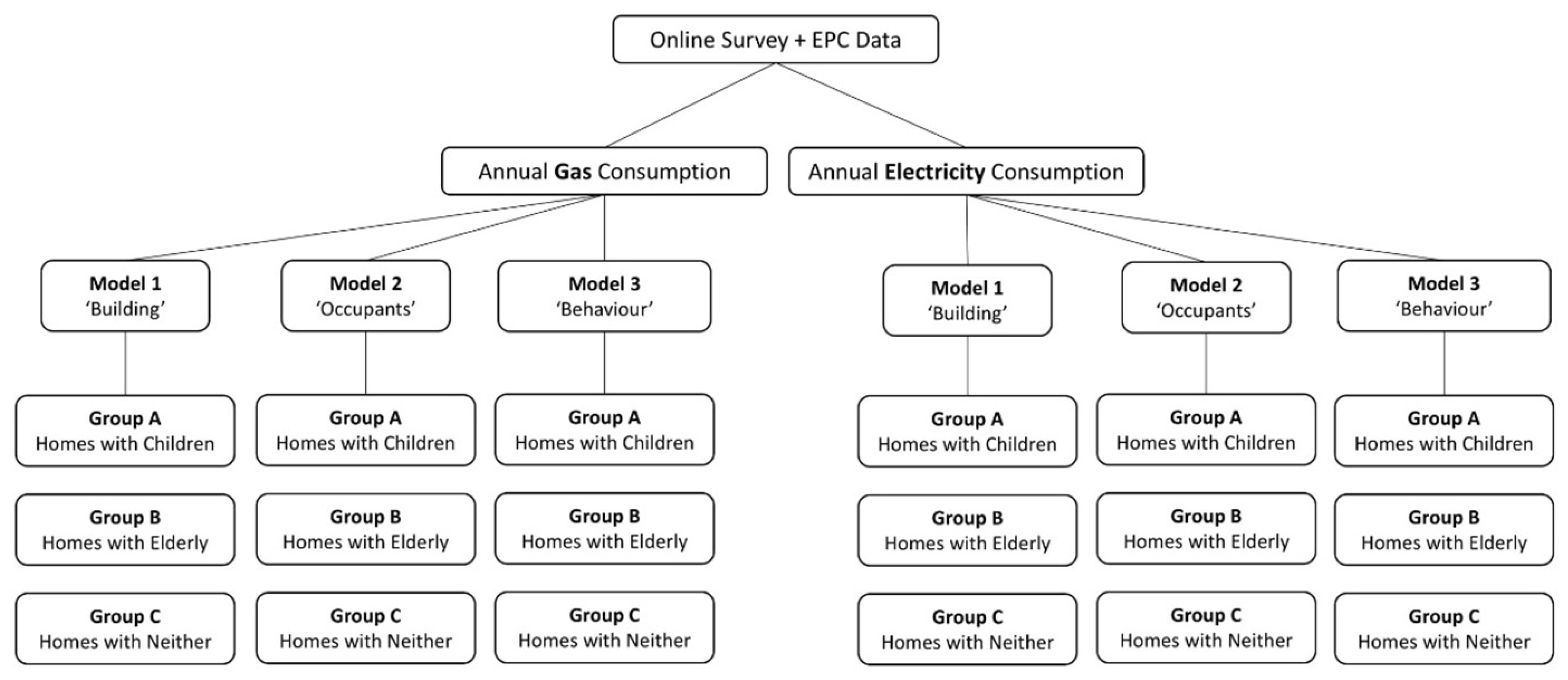
The dataset was divided into three household groups: Group A. Homes with children (n = 1576), Group B. Homes with elderly (n = 436), and Group C. Homes with neither children nor elderly (n = 2330). Gas and Electricity consumption are the two dependent variables analysed in this study; the same analysis was undertaken for each of these consumption data. The analysis undertook three Lasso Regression Models, each looking at the 3 different aforementioned models; ‘Building’, ‘Occupants’ and ‘Behaviour’. The models were repeated for the three household groups, allowing comparisons between groups and between gas and electricity consumption. The data analysis framework is summarised in Figure 1.
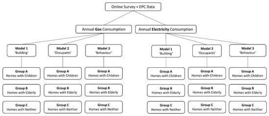
Figure 1.
Data analysis framework.
First, the analysis reviewed each variable through descriptive analysis, identifying outliers. Then, an analysis of variance (ANOVA) of Electricity and Gas consumption between the three groups was carried out. This was followed by Lasso regression analysis to identify which variables are strong predictors of consumption for each group.
Lasso regression (Least Absolute Shrinkage and Selection Operator) was used as it not only produces data on predictors but also mitigates any multicollinearity—when several variables within a regression model may be highly correlated, which is detrimental to interpretation and analysis [26]. Lasso accomplishes this by “introducing a penalty term in the model and shrinking the regression coefficients to zero, allowing the model to achieve a higher level of accuracy when compared to traditional models” [52]. The regression values within Lasso may remain positive or negative depending on whether the correlation is positive or negative; the more the value is shrunk (the closer it gets to zero), the less powerful it is as a predictor. K-fold cross-validation was first used to find the optimal lambda value for each of the Lasso regressions; for the 3 groups, 3 models and 2 m reading types (18 tests in total). The Lasso regressions were then completed using these lambda values.
Finally, within each group, relationships between each variable and consumption were tested using either Spearman-Rank test or Kruskal–Wallis test depending on the variable type.
3. Results
3.1. Exploring the Difference in Annual Electricity and Gas Consumption between Household Groups
The electricity and gas consumption appears to be very similar between household groups, see Figure 2. However, there are statistically significant differences between household groups for gas consumption (H(2) = 2; p = 2.2 ) and electricity consumption (H(2) = 2; p = 4.197 ). This is to be expected and follows existing literature suggesting homes with more occupants, or with elderly or young family members consume more energy, usually to maintain thermal comfort [42].
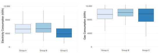
Figure 2.
Annual Electricity (on the left) and Annual Gas consumption (on the right) for the three household groups.
Group C (with neither) has the lowest median and mean of the three groups which is also to be expected [39]. Again, following the pattern seen in the literature, Group B (with elderly) has the highest median and mean with elderly relatives usually requiring more energy consumption to maintain comfort levels and remain healthy [40].
3.2. Identifying the Predictors of Annual Electricity and Gas Consumption for Each Household Group
Results from the Lasso Regression on electricity and gas consumption show a difference between the final predictors within each group (see Table 3). The two strongest predictors are highlighted in Table 3; these are the two predictors with absolute values furthest from 0. These results are explored in the following sections, starting with ‘Model 1—Electricity’ and ‘Model 1—Gas’, then ‘Model 2—Electricity’ and ‘Model 2—Gas’, and finally ‘Model 3—Electricity’ and ‘Model 3—Gas’.
Table 3.
Lasso regression analysis results.
Within ‘Model 1—Electricity’, ‘Property Type’ is one of two the most powerful variables for all three household groups. For Group B, it is the most powerful predictor. ‘Property Type’ is also the most consistently powerful result of any variable within any group or model, suggesting that the type of property will be one of the strongest determining factors of energy consumption. ‘Main Fuel’ is then the second most powerful variable for both Group A and Group C, but has been reduced to zero for Group B, which interestingly has instead ‘Wall Type’ as the second most powerful variable, this has been reduced to zero for both Group A and C. Interestingly, ‘Window Energy Efficiency’ is only powerful for Group C and ‘Current Energy Efficiency’ which is simply the EPC Score of the property, shows very low levels of prediction power. EPC is the national standard to test how much energy a home will consume, yet other predictors are more powerful.
Within ‘Model 1—Gas’, ‘Property Type’ is again the most powerful variable for two of the three household Groups; A and C. Yet it has been reduced to zero in Group B. ‘Wall Description’ sees a small increase from the Electricity Model to the current Gas Model and again is one of the top two predictors for Group B, suggesting that this variable is particularly important for predicting overall energy consumption in homes with elderly occupants. The variable ‘Window Energy Efficiency’ also sees an increase in levels of power from Electricity to Gas models for two household groups A and C, becoming the second most powerful variable for Group A. This suggests that the performance of windows is more important for electricity saving than for gas saving for households with children. The variable ‘Main Fuel’ remains one of the top two predictors for Group C, but has now been reduced to zero for Group A and remains at zero for Group B. Interestingly, the variable ‘Current Energy Efficiency’ has now become the most powerful predictor for Group B and is now also slightly more powerful for the two other groups. This reaffirms that SAP is more based on gas consumption, not electricity, overall consumption or unregulated energy.
Within ‘Model 2—Electricity’, there is slightly less consistency between which variables are powerful when compared to ‘Model 1—Electricity’. The variable ‘Number of Occupants’ is the most powerful predictor for both Group A and C, but has reached zero for Group B. It would be expected that those homes with more occupants would consume more energy, but it appears that this variable is not powerful enough to be the case for homes with elderly. Groups A and B show ‘Please state your gender’ as a strong predictor, which could show some interesting results after further analysis. ‘Do you own your own home?’ is then one of the strongest two predictors for Group C. Whilst the variable ‘How long have you lived in your home?’ is a strong predictor for Group B only.
Within ‘Model 2—Gas’, the variable ‘Do you own your home?’ is a strong predictor for all three groups. This may suggest that the difference in consumption between those owning their homes and those renting could be substantial, potentially because of the improvements one can make on their own home relative to rented accommodation. The variable ‘Number of occupants’ is again a strong predictor for Group C, and the variable ‘Please state your gender’ is again for Group A, but both variables see decreases within other groups within the model. The variable ‘How long have you lived in your home?’ is a strong predictor for Group B once again, suggesting that this could be a reliable predictor for overall energy consumption.
Within ‘Model 3—Electricity‘, Group B has had all but one variable reduced to zero through the Lasso Regression. The variable ‘Who has the last word with heating decisions’ is the only variable to remain a predictor. This variable is also a low-scoring predictor for the two other groups. The variable ‘Main Heat Source’ is a strong predictor for both Groups A and C, as well as the variable ‘Do you use additional electric heating in the winter?’. This result is unexpected as the literature would suggest that households with elderly more often use additional heating sources to spot heat individual rooms [41].
Within ‘Model 3—Gas‘, the variable ‘What time is heating on?’ has increased in power across all three groups (from Model 3 Electricity to Model 3 Gas) and become a top predictor for Group B. This may suggest that households with elderly abide by different heating time schedules, likely to maintain the thermal comfort of those elderly which falls in line with literature [41]. Only one variable within ‘Model 3—Gas’ is the same as ‘Model 3—Electricity’, ‘Do you use additional electric heating in the winter?’, and it has remained a strong predictor for Group A. Interestingly, the variable ‘Heating Schedule’ has also increased in power (from Model 3 Electricity to Model 3 Gas) and is now a strong predictor for Group C, but reduced to zero for Group B, where one would expect a similar increase for the reasons suggested above.
3.3. Exploring Differences with the Predictors of Annual Electricity and Gas Consumption for Each Household Group
The relationship between the outcome of ‘electricity and gas consumption’ and the predictors within each household group are reviewed by applying either Spearman Rank test or Kruskal–Wallis test depending on the nature of the data (discrete or continuous). The highlighted results in Table 4 are those that show a significant difference between groups. As above, these results are explored in the following sections, starting with ‘Model 1—Electricity’ and ‘Model 1—Gas’, then ‘Model 2—Electricity’ and ‘Model 2—Gas’, and finally ‘Model 3—Electricity’ and ‘Model 3—Gas’.
Table 4.
Spearman Rank test and Kruskal–Wallis test analysis results.
Within ‘Model 1—Electricity’, no variables show a significant difference between groups for Group B, but ‘Total Floor Area’ and ‘Main Fuel’, both show significant differences between groups for Group A and C, suggesting that these two variables may be the most important for gauging energy use in the home. Group C, electricity consumption shows a significant difference between groups for the variables ‘Property Type’ and ‘Local Authority’, the latter suggesting the local climate can play a role in electricity consumption.
The ‘Model 1—Gas’ results vary considerably compared to the electricity model; both ‘Total Floor Area’ and ‘Property Type’ show a significant difference between groups for all three household groups with ‘Wall Description’ and ‘Window efficiency’ showing significant difference between groups for groups A and C. Group C shows a significant difference between groups for all variables.
Eight of the 18 tests of ‘Model 2—Electricity’ show significant differences between groups for all three household groups. Group B has identical results to ‘Model 1 -Electricity’, as it shows no difference within any variable. Groups A and C both show significant differences within ‘Number of Occupants’ and within ‘How many years living in the home’. The variable ‘Number of Children’ shows a significant difference between groups for Group A, but not for Groups B and C. Finally, ‘Gender’ shows a significant difference between groups for Group C only.
Within ‘Model 2—Gas’, the variable ‘Do you own your home’ is the only variable to show a significant difference between groups for all three household types, suggesting again that there may be a benefit from the freedom that owning one’s home brings in terms of mitigating gas consumption. It would be expected that the variable ‘Number of Occupants’ would have a strong relationship with gas consumption, but it only shows statistically significant results for Group C. This household type is only made up of single people or couples, potentially meaning the change from one to two occupants plays a larger role than the following change from more than two occupants. The variables ‘Gender’ and ‘How many years living in the home’ show significant differences between groups for two out of three household groups. The variable ‘Person Age’ only shows a significant difference between groups for Group C.
Within ‘Model 3—Electricity’, the variable ‘Set Room Temperature’ shows a significant difference between groups for all three household groups. This is to be expected as space heating in domestic properties is the largest energy consumer [5]. However, the majority of space heating in this study is gas-powered, thus this may require further analysis. The variables ‘Main Heat Source’, ‘Heating Schedule’, ‘Time Heating is on’, ’Action when Felling Cold’ and ‘Additional Heating?’ all show significant differences between groups for household groups A and C. Group B again shows very few significant differences for the variables included in this analysis.
The same can be said for Group B in ‘Model 3—Gas’; there is no significant difference between groups for any variable. Yet, Group C shows a significant difference between groups for all variables. Group A in ‘Model 3—Gas’ has almost identical results to Group A in ‘Model 3—Electric’; showing only one change, no longer having a significant difference between groups for the variable ‘Main Heat Source’.
4. Discussion
The first step of the analysis was to review the variability in electricity and gas annual consumption between household groups; ‘Group A—With Children’, ‘Group B—With Elderly’ and ‘Group C—With Neither’. Although little difference in central tendency was observed, there was a significant difference between groups, with households with elderly residents consuming more energy. This analysis led to the review of the energy consumption predictors of each household group.
From the Lasso regression analysis, ‘Model 1—Building’ results show that the variable ‘Property Type’ is the strongest predictor for both electricity and gas consumption, often reaching scores of a magnitude of ten times larger than other variables. Importantly, this result is observed across all three household groups. This falls in line with the literature, which showed physical building variables have the largest effect on domestic energy consumption [26], but it is important to approach energy consumption mitigation from other angles, especially when property type cannot be changed or improved in around half of the UK dwellings (e.g., rented accommodation, historic properties, etc.) [53].
It is apparent from the results of both the Lasso regression analysis and the inferential analysis, that variables relating to dwelling ownership seem to play a large role in terms of energy consumption. The variable ‘Do you own your home?’ is a strong predictor of the Lasso regression analysis for four out of six groups, and shows significant differences between groups for five out of six household groups within the inferential analysis. Similarly, the variable ‘Length of time in home’ is a strong predictor of the Lasso regression analysis for two out of six groups, and shows significant differences between groups for four out of six household groups within the inferential analysis. Literature considered the ownership of homes an important aspect of mitigating energy use [26].
The results of this analysis appear to fall in line with points raised by other studies; that those who own their home can upgrade their envelopes or systems over time, thus reducing their energy consumption compared to similar dwellings that are not owned by occupants. This difference between rented/ownership status, and thus the difference between who pays and who benefits from building upgrades, is known as the ‘Split Incentive Effect’. Kristrom et al. (2015) found that “owners are substantially more likely to have access to energy-efficient technologies and better insulation”, thus could reduce energy consumption more than renters [54]. This issue is currently being discussed at the national level, with potential plans to enforce a mandatory EPC rating ‘C’ for all rented dwellings by 2025 [55]. This would require improvements to the buildings’ envelopes and systems/technologies, which this study’s result also suggests being the most powerful influencers and thus sensible improvements to be made first.
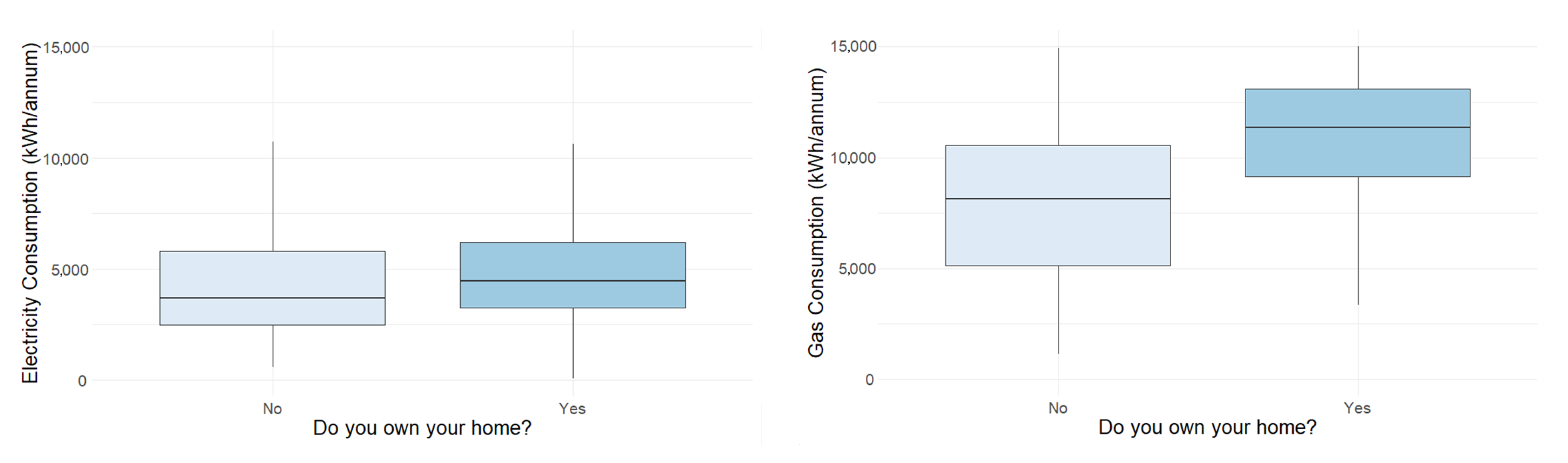
In the UK, 63% of households own their place of residence [53], but within this survey, 75% (n = 3688) of participants stated they owned their home. This higher rate demonstrates how the sample is not truly reflective of the UK. It can be expected that, with this higher rate of ownership along with the aforementioned opportunities homeowners have to implement upgrades, energy consumption may be lower in the survey than that of the UK average household. However, this study’s results show the opposite with the owned group representing larger average energy consumption than non-owners (both for gas and electricity), see Figure 3. This may be because other variables are affecting energy consumption. The average floor area in the sample is 117sqm, whereas the UK average is lower at 97sqm [55]. This will likely mean that energy consumption is higher within the study results than would be expected based on UK averages. Similarly, the average income for a household in the UK is £35K [56], whereas 40% of the sample falls within the ‘greater than £60K’ category. This implies that participants have on average more disposable income and are less constrained to consume energy, thus the energy consumption data is higher than expected.
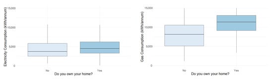
Figure 3.
All household groups, variable ‘home ownership’ (Yes/No) for electricity consumption (on the left) and gas consumption (on the right).
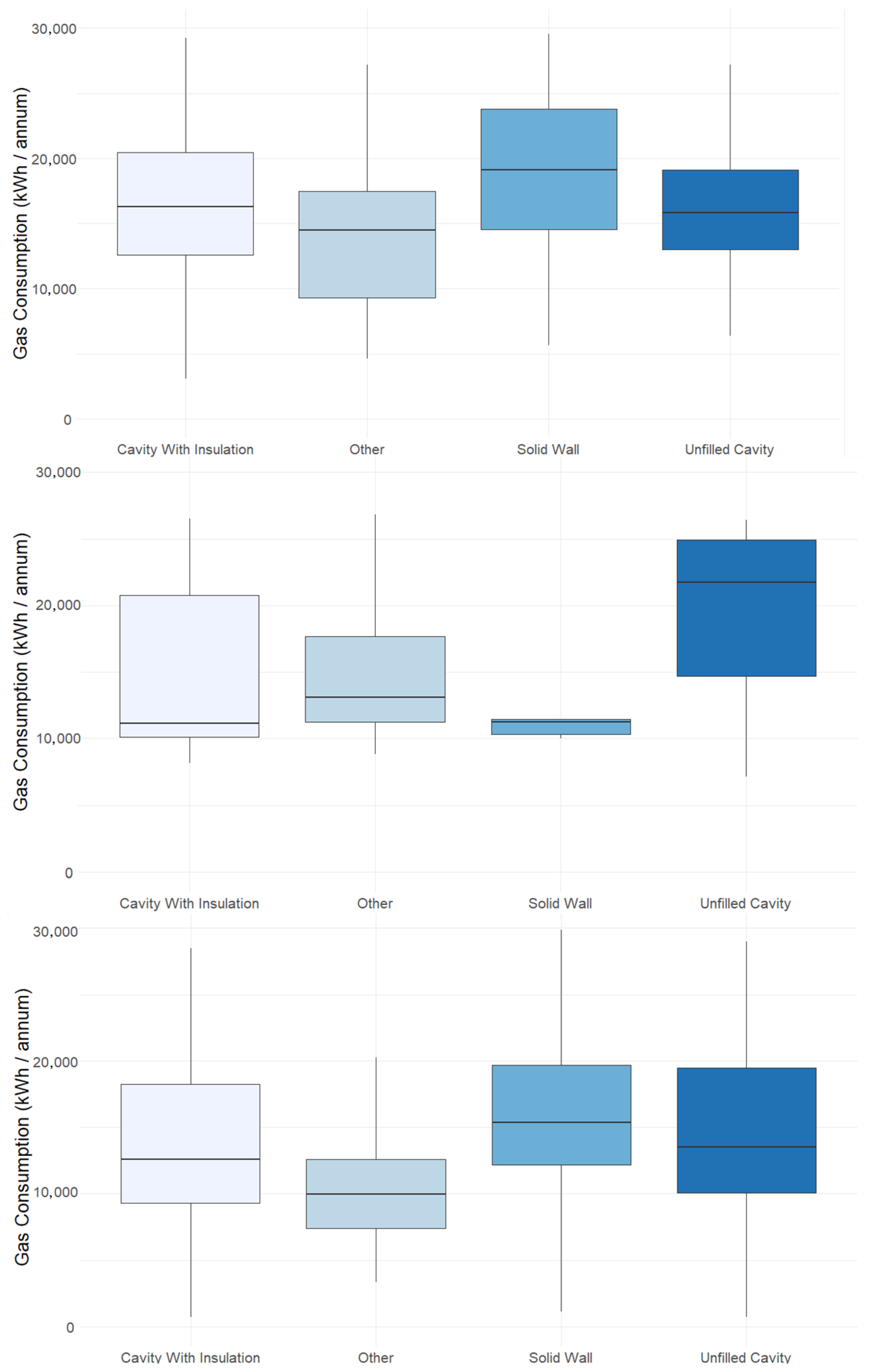
This study and the review of literature have highlighted that variables such as ‘dwelling age’ are unreliable for a study such as this because this variable does not allow for dynamic measuring, it only refers to a single point of measurement in time. However, the variable ‘Wall Description’ is a current measurement of a dwelling that also encompasses any changes that may have been made to the property. Thus, it may be a better representation of building performance. The Lasso regression analysis shows that the variable ‘Wall Description’ is a predictor of gas consumption for all household groups and a strong predictor for Group B, but it is less powerful within the electricity models, with it only being a predictor for Group B. The skew to gas over electric may suggest that the wall types are more influenced by aspects such as heating (which is predominantly gas-sourced). In the future, this may change with the gradual transition to electric heating. The result, that wall type is only a strong predictor in homes with elderly, may also be based on heating use, but because of the higher temperature levels (and longer heating periods) that the elderly require to maintain thermal comfort as discussed earlier and put forward by Pais-Magalhaes et al. (2022). Figure 4 shows gas consumption vs. wall types for groups A, B and C, respectively, and that Group B (with Elderly) does not show the same pattern as groups A and C, which are very similar [42].
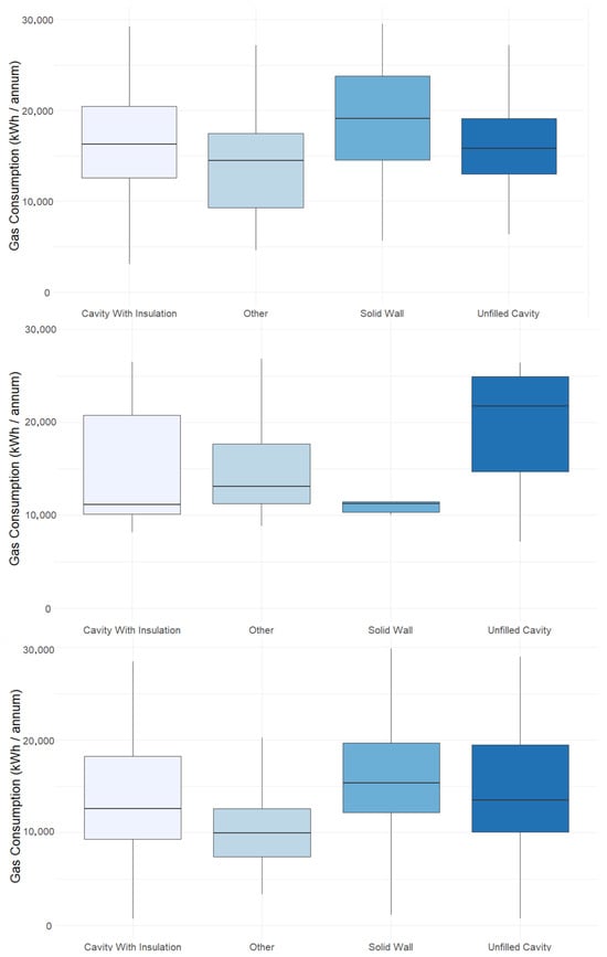
Figure 4.
Variable ‘Wall construction’ vs. Gas consumption in kWh/annual for ‘Group A—With Children’ (top), ‘Group B—With Elderly’ (middle) and ‘Group C—With Neither’ (bottom).
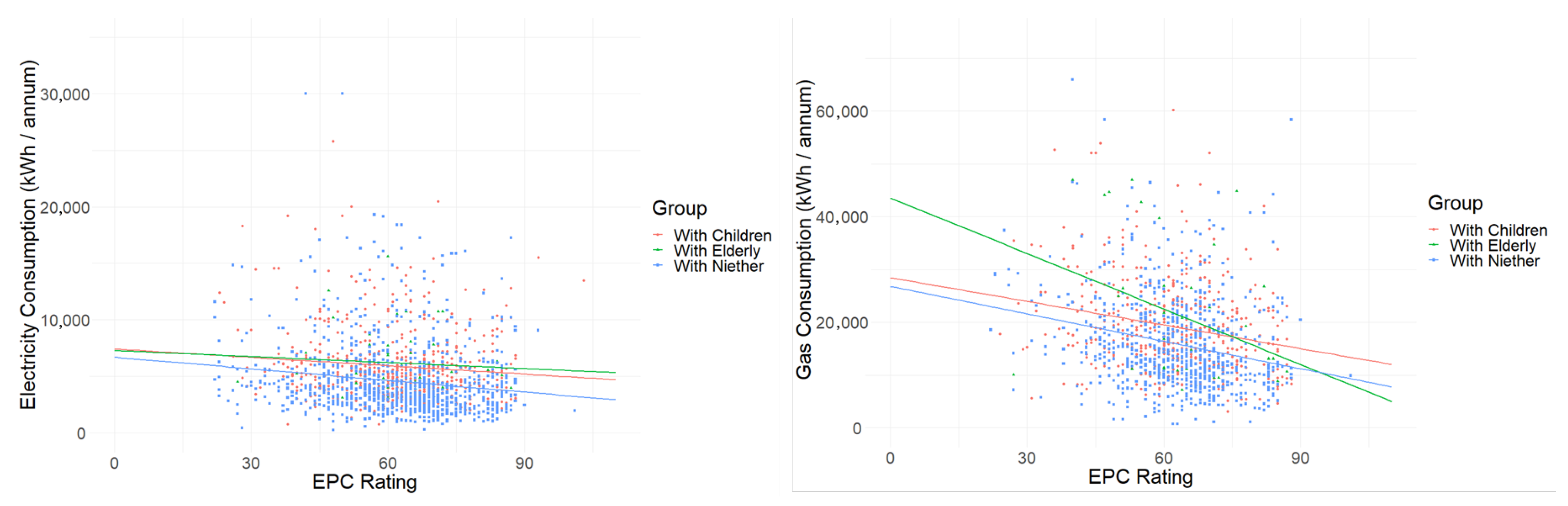
On the variable ‘current energy efficiency’, It could be expected that the SAP rating would be the strongest predictor and show the strongest relationship with energy consumption as this is the tool used by the UK government to predict energy consumption. However, the results show that the variable is only a strong predictor for Group B gas consumption. Yet, it shows a significant difference between groups with all but one group within the inferential analysis (Spearman Rank). The difference between the two sets of results would suggest further analysis is required. This does however reinforce the idea that the EPG may be at least partly due to variables not considered within SAP, such as occupant behaviour and unregulated energy consumption as previously discussed. More research is required that consistently measures similar variables (both for modelling and real-world measuring). The results also call into question the validity of any modern EPC as the score is marketed as a true representation of energy consumption. The mean average EPC rating for the participant group is 62 (E), which is very similar to the national average of 60 [32]. This variable is far closer to the UK average than many of the others analysed in this study. It could be expected that with higher levels of ownership and income, homes in the sample would achieve a higher-than-average EPC rating. Figure 5 shows EPC Results against gas and electricity consumption. The regression lines suggest that the higher the score, the less energy is consumed, which is to be expected, but the shallowness of the line suggests the differences between the scores are small (see Table 5).
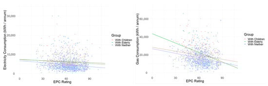
Figure 5.
Variable ‘current energy efficiency’(EPC rating) vs. electricity consumption (on the left) and vs. gas consumption (on the right), for ‘Group A—With Children’(red line), ‘Group B—With Elderly’ (green line) and ‘Group C—With Neither’ (blue line).
Table 5.
Summary of Results from variables ‘current energy efficiency’(EPC rating) vs. consumption (gas and electricity).
It can be seen from Figure 5 that the regression lines in the electricity graph maintain the same position as the EPC rating increases. Homes with elderly consistently consume more electricity. but as the EPC improves, the gap between the three regression lines increases, suggesting that having dependents in the home limits the potential energy saving that may come by living within a high-performing home. The gas consumption graph on the right shows that having elderly in a poor-performing home will mean gas consumption is significantly higher than the two other groups, but this improves strongly as the EPC improves until having elderly in the home means that energy consumption will be less than the other two groups (A and C). The two regression lines of groups A and C maintain a consistent position and steepness to each other throughout the EPC rating range.
The results from the variables such as ‘Number of Occupants’ and ‘Floor Area’ are as expected; when there are more bodies to feed, wash and maintain comfort for, energy use increases [26]. Similarly, when there is a larger home to heat then overall energy consumption of gas and electricity increase. the variable ‘Number of Occupants’ is a strong predictor for ‘Electricity—Group A’, ‘Electricity—Group C’ and ‘Gas—Group C’, it is also a predictor for ‘Gas—Group A’.
The variable ‘Gender’ is also important within surveys, especially regarding aspects such as heating. Males generally require a lower temperature to maintain thermal comfort [57] or genders may have different roles in the home which means they behave in different ways or have knowledge of differing aspects of energy in the home [58]. Within this survey, the variable ‘Please state your gender’ is a strong predictor for three of the six household groups (‘Electricity—Group A’, ‘Electricity—Group B’ and ‘Gas—Group A’). The gender in the sample was 30% Female (n = 1499), 57% Male (n = 2815) and 13% Other (n = 639).
Continuing with occupant factors, the variable ‘Who has the last word on heating decisions?’ is a strong predictor for ‘Electricity—Group B’ and is only disregarded in one of the six household groups (‘Gas—Group B’). Thus, this variable can be considered an important aspect. 34% (n = 1700) of participants stated they have the final word, 44% (n = 2202) stated it was equally shared, 6% (30) stated their partner had the final say and circa 20% stated ‘other’ or did not answer.
It is important to remember that both gas and electricity consumption data within this study were taken directly from meter readings, including regulated and unregulated uses from water heating, space heating and more. Thereby, singularly looking at the main heating source as a variable may not portray a true representation of energy in the home. Having said that, within the Lasso Regression analysis, the variable is a strong predictor for ‘Electricity—Group A’, ‘Electricity—Group C’, and ‘Gas—Group A’, suggesting when there are elderly relatives in the home (Group B), the heating source is not an important factor in predicting energy consumption, but when there are children in the home (Group A), the main heat source is. This is the opposite result when compared to the variables ‘How many years lived in home’ and ‘wall description’, which appear to be far more powerful predictors for homes with elderly.
The ‘Additional heaters used’ variable, which would be expected to be a powerful predictor for group B (with elderly) based on the literature, interestingly is a top predictor for the groups without elderly in the home.
5. Conclusions
5.1. Summary of Findings
Domestic energy consumption is a significant and highly complicated issue, dependent on an array of variables and influences. This study aimed to gain insight into the aspects that influence gas and electricity usage in three different household groups: homes with children, homes with elderly and homes with neither older nor younger generations. Using Lasso Regression analysis on three different models of variables (Building, Occupants and Behaviour), the results identified the most powerful predictors of energy consumption within each group.
Property Type was found to be the most powerful predictor of both gas and electricity consumption across the six groups (three for electricity and three for gas), fundamentally suggesting that the physical building should be the first variable considered when discussing energy consumption in homes. However, this is one of several factors that cannot be changed—a detached dwelling cannot be changed into a flat. The first significant conclusion from this work follows that if the most significant variable cannot be altered, then it reaffirms the idea that less studied aspects such as occupant behaviour should be considered more in policies addressing change in reduction in energy consumption. Improving occupant energy behaviour could be one of the most effective ways to achieve a reduction in energy consumption in dwellings that can have little else improved. Although this paper discusses only several factors occupants control, it has shown that some may act as powerful predictors, thus with more evidence and modelling could be applied to potential future energy model predictions such as the design stage SAP.
Homeownership was the second most powerful predictor, showing a significant relationship with five of the six groups. Interestingly, homeowners used slightly more electricity and gas than non-owners, which contrasts with existing literature suggesting that homeowners typically retrofit their homes to improve energy efficiency. However, the sample’s higher-than-average levels of homeownership, education, income, retirement rates, and house size may explain these results.
The variables ‘Main Fuel Type’, ‘Number of Occupants’, ‘Gender’ and ‘Additional Heaters’ are the next most powerful predictors, each being one of the two highest scoring results across three total of six groups. Only the first of which is considered within the SAP calculation, the latter are not, yet appear to be important variables that can be used to predict energy consumption in the home. This could be more evidence to inform the EPG. Current Energy Efficiency (EPC Rating) as a variable is also only a top predictor in one of the six groups (elec B) but is used nationally as the main comparison of energy consumption between dwellings. This paper has produced results that add to supporting evidence that shows SAP needs to be updated to fall in line with the way homes are used today. Of course, more research and accurate models are still required, but if SAP included both regulated and an accurate assumption of unregulated energy use (possibly dependent on the occupant demographics within the property—as this paper investigates), it would support reducing the energy performance gap.
The variables ‘Set room temperature’ and ‘Floor area’ show significant relationships with more groups than any other variable, but are not top predictors within any group. Having said that, they still show results within the Lasso regression analysis, rather than being reduced to 0, thus they can still be used to predict energy consumption. These two variables are intrinsically linked to space heating; the most influential consumer of energy in the home and one that can be completely controlled by the occupiers. Is there a potential for improvement in how occupants use their heating systems? The government, or energy providers, could target users with campaigns that promote more conscientious use of heating systems in homes, helping in the reduction of energy consumption in the UK.
Comparing the three models, Building Variables should be the first part of any decision that aims to improve energy use. For example, a fabric-first approach to retrofitting would be more influential than improving systems or technologies within the home. But these, along with occupant behaviours, are also important influencers that should be encouraged to be considered more often [59]. This is especially important within dwellings that are unable to be retrofitted in traditional ways such as insulation improvements.
The results from this study seem to show that occupant behaviour not only plays an important role in energy consumption in the home but also should be incorporated into future alterations to energy models. It is expected that more research needs to take place in this area before this is the case, but with the energy performance gap being as prevalent as ever, it is vital that all areas are investigated with the aim of reducing it.
5.2. Limitations of Study and Future Research
There are several important aspects to note regarding the limitations of this study. The participant sample is not fully representative of the UK population, with higher-than-average figures for household income, home size, homeownership rates, education levels, and EPC ratings.
Although the gas and electricity metering data were automatically collected, and the building data were extracted from the EPC certificates, most of the other data were self-reported by participants. This not only leads to human error in occurrences but also an internal bias. Surveys were also completed by one occupant within the home, which means inherently there may be some bias. The participants would have given answers on their own behaviours over other occupants in the home. Also, there may be some bias in the response, as participants may have answered inaccurately or falsely to appear better or simply did not know the true answer and gave their opinion. Previous research by Gauthier, (2015) has shown that when asked about their behaviours, participants will often suggest they behave differently than they do in real life [60].
The gas and electricity meter readings have been collected over one year, which may have been a hotter or colder than average year. Heating Degree Days (HDD) are a way of balancing data such as this to make it comparable to other years and could be used if further analysis is required.
This survey was carried out before 2022, UK energy bills have increased substantially over the past two years and thus the economic factors of today’s climate may have led to some participants behaving and data differently.
This study has shown that occupant behaviour, although not the most influential factor, should still be considered when attempting to model or predict energy consumption in the home. It is especially important during the design stage as a method of mitigating the energy performance gap that has become apparent in recent years. Although not a true representation of the UK, this study suggests that some demographic or occupant behaviour factors (such as the use of a secondary heating system) could not only be used as predictors for electricity and gas consumption but may be as accurate as traditional predictors such as EPC scores. The inherent inclusion of unregulated energy within this study (by using meter data) has shown how influential it can be and how future predictions should aim to include this aspect.
Author Contributions
G.S.: formal analysis, visualization and writing original draft preparation. S.G., P.J. and S.S. are responsible for conceptualization, methodology, data curation and supervision. All authors have read and agreed to the published version of the manuscript.
Funding
The work is supported by the EPSRC Project: Residential Heat as an Energy System Service (LATENT) (EP/T023074/1).
Data Availability Statement
Data is not aviliable to public as BREACHES ethics application.
Acknowledgments
This work is part of the activities of the Energy and Climate Change Division and the Sustainability Energy Research Group at the University of Southampton (www.energy.soton.ac.uk, 1 September 2024). The work is supported by the EPSRC Project: Residential Heat as an Energy System Service (LATENT) (EP/T023074/1) with acknowledgement given to the wider project team for the collection and sharing of data used for the purpose of this study.
Conflicts of Interest
The authors declare no conflict of interest.
References
- UK Government. Climate Change Act 2008 (c.27). In United Kingdom Public General Acts; UK Government: London, UK, 2024; Volume 2050. [Google Scholar]
- HM Government. UK Enshrines New Target in Law to Slash Emissions by 78% by 2035. Available online: https://www.gov.uk/government/news/uk-enshrines-new-target-in-law-to-slash-emissions-by-78-by-2035 (accessed on 24 May 2022).
- ONS. Digest of UK Energy Statistics Annual Data for UK. 2024. Available online: https://www.gov.uk/government/statistics/digest-of-uk-energy-statistics-dukes-2024 (accessed on 1 February 2024).
- World Population Review. Energy Consumption by Country 2023. Available online: https://worldpopulationreview.com/country-rankings/energy-consumption-by-country (accessed on 24 May 2022).
- Reguis, A.; Vand, B.; Currie, J. Challenges for the transition to low-temperature heat in the UK: A review. Energies 2021, 14, 7181. [Google Scholar] [CrossRef]
- Ofgem. Feed-in Tariffs (FIT) Scheme Closure. Available online: https://www.ofgem.gov.uk/environmental-and-social-schemes/feed-tariffs-fit/feed-tariffs-fit-scheme-closure (accessed on 24 May 2022).
- HM Government. Code for Sustainable Homes-Withdrawn. Available online: https://www.gov.uk/government/publications/code-for-sustainable-homes-technical-guidance (accessed on 24 May 2022).
- Constable, J. Energy Efficiency: Lessons from the Green Deal and Energy Company Obligation. Available online: https://www.netzerowatch.com/all-news/energy-efficiency-lessons-from-the-green-deal-and-energy-company-obligation (accessed on 24 May 2022).
- Broad, O.; Hawker, G.; Dodds, P.E. Decarbonising the UK residential sector: The dependence of national abatement on flexible and local views of the future. Energy Policy 2020, 140, 111321. [Google Scholar] [CrossRef]
- HM Government. Apply for the Boiler Upgrade Scheme. Available online: https://www.gov.uk/apply-boiler-upgrade-scheme (accessed on 24 May 2022).
- Nat Geo. What is COP 26. Available online: https://www.natgeokids.com/uk/discover/science/nature/what-is-cop26-glasgow/ (accessed on 24 May 2022).
- Bolton, P. Domestic Energy Prices Summary; House of Commons Library: London, UK, 2024; pp. 1–61. [Google Scholar]
- De Wilde, P. The gap between predicted and measured energy performance of buildings: A framework for investigation. Autom. Constr. 2014, 41, 40–49. [Google Scholar] [CrossRef]
- Xu, X.; Xiao, B.; Li, C.Z. Critical factors of electricity consumption in residential buildings: An analysis from the point of occupant characteristics view. J. Clean. Prod. 2020, 256, 120423. [Google Scholar] [CrossRef]
- Mitchell, R.; Natarajan, S. UK Passivhaus and the energy performance gap. Energy Build. 2020, 224, 110240. [Google Scholar] [CrossRef]
- Mahdavi, A.; Berger, C.; Amin, H.; Ampatzi, E.; Andersen, R.K.; Azar, E.; Barthelmes, V.M.; Favero, M.; Hahn, J.; Khovalyg, D.; et al. The role of occupants in buildings’ energy performance gap: Myth or reality? Sustainability 2021, 13, 3146. [Google Scholar] [CrossRef]
- Bardsley, N.; Büchs, M.; James, P.; Papafragkou, A.; Rushby, T.; Saunders, C.; Smith, G.; Wallbridge, R.; Woodman, N. Domestic thermal upgrades, community action and energy saving: A three-year experimental study of prosperous households. Energy Policy 2019, 127, 475–485. [Google Scholar] [CrossRef]
- UKERC. The Rebound Effect. Available online: https://ukerc.ac.uk/project/the-rebound-effect-report/#:∼:text=An%20example%20of%20a%20rebound,bill%20towards%20an%20overseas%20holiday (accessed on 24 May 2022).
- Huebner, G.M.; Watson, N.E.; Direk, K.; McKenna, E.; Webborn, E.; Hollick, F.; Elam, S.; Oreszczyn, T. Survey study on energy use in UK homes during COVID-19. Build. Cities 2021, 2, 952–969. [Google Scholar] [CrossRef]
- Anderson, B.; James, P. COVID-19 lockdown: Impacts on GB electricity demand and CO2 emissions. Build. Cities 2021, 2, 134–149. [Google Scholar] [CrossRef]
- Eyre, N.; Baruah, P. Uncertainties in future energy demand in UK residential heating. Energy Policy 2015, 87, 641–653. [Google Scholar] [CrossRef]
- Guerra-Santin, O.; Itard, L. Occupants’ behaviour: Determinants and effects on residential heating consumption. Build. Res. Inf. 2010, 38, 318–338. [Google Scholar] [CrossRef]
- Bresa, A.; Zakula, T.; Ajdukovic, D. Occupant-centric control in buildings: Investigating occupant intentions and preferences for indoor environment and grid flexibility interactions. Energy Build. 2024, 317, 114393. [Google Scholar] [CrossRef]
- Nord, N.; Tereshchenko, T.; Qvistgaard, L.H.; Tryggestad, I.S. Influence of occupant behavior and operation on performance of a residential Zero Emission Building in Norway. Energy Build. 2018, 159, 75–88. [Google Scholar] [CrossRef]
- Guerra-Santin, O.; Tweed, C.; Jenkins, H.; Jiang, S. Monitoring the performance of low energy dwellings: Two UK case studies. Energy Build. 2013, 64, 32–40. [Google Scholar] [CrossRef]
- Huebner, G.M.; Hamilton, I.; Chalabi, Z.; Shipworth, D.; Oreszczyn, T. Explaining domestic energy consumption—The comparative contribution of building factors, socio-demographics, behaviours and attitudes. Appl. Energy 2015, 159, 589–600. [Google Scholar] [CrossRef]
- Sharpe, R.A.; Thornton, C.R.; Nikolaou, V.; Osborne, N.J. Higher energy efficient homes are associated with increased risk of doctor diagnosed asthma in a UK subpopulation. Environ. Int. 2015, 75, 234–244. [Google Scholar] [CrossRef]
- Aragon, V.; James, P.A.; Gauthier, S. The influence of weather on heat demand profiles in UK social housing tower blocks. Build. Environ. 2022, 219, 109101. [Google Scholar] [CrossRef]
- Ben, H.; Steemers, K. Household archetypes and behavioural patterns in UK domestic energy use. Energy Effic. 2018, 11, 761–771. [Google Scholar] [CrossRef]
- Baker, P.; Blundell, R.; Micklewright, J. Modelling Household Energy Expenditures Using Micro-Data. Econ. J. 2017, 99, 720–738. [Google Scholar] [CrossRef]
- Chen, F.; Zu, X.; Brigs, M.; Nelson, H. Exploring the factors that influence energy use intensity across low-, middle-, and high-income households in the United States. Energy Policy 2022, 168, 113071. [Google Scholar] [CrossRef]
- ONS. Energy Efficiency of Housing in England and Wales. 2022. Available online: https://www.ons.gov.uk/peoplepopulationandcommunity/housing/articles/energyefficiencyofhousinginenglandandwales/2022 (accessed on 24 May 2022).
- HM Government. Conservation of Fuel and Power (Part L). The Building Regulations, 16.1-16.128; Technical Report; HM Government: London, UK, 2017.
- BRE. BREDEM 2012—A Technical Description of the BRE Domestic Energy Model; BRE: Watford, UK, 2013; p. 37. [Google Scholar]
- Firth, S.K.; Lomas, K.J.; Wright, A.J. Targeting household energy-efficiency measures using sensitivity analysis. Build. Res. Inf. 2010, 38, 25–41. [Google Scholar] [CrossRef]
- Amin, R.; Teli, D.; James, P.; Bourikas, L. The influence of a student’s ’home’ climate on room temperature and indoor environmental controls use in a modern halls of residence. Energy Build. 2016, 119, 331–339. [Google Scholar] [CrossRef]
- Verbruggen, S.; Delghust, M.; Laverge, J.; Janssens, A. Habitual window opening behaviour in residential buildings. Energy Build. 2021, 252, 111454. [Google Scholar] [CrossRef]
- Bardazzi, R.; Pazienza, M.G. When I was your age: Generational effects on long-run residential energy consumption in Italy. Energy Res. Soc. Sci. 2020, 70, 101611. [Google Scholar] [CrossRef]
- Zhu, P.; Lin, B. Do the elderly consume more energy? Evidence from the retirement policy in urban China. Energy Policy 2022, 165, 112928. [Google Scholar] [CrossRef]
- Estiri, H.; Zagheni, E. Age matters: Ageing and household energy demand in the United States. Energy Res. Soc. Sci. 2019, 55, 62–70. [Google Scholar] [CrossRef]
- Kane, T.; Firth, S.K.; Lomas, K.J. How are UK homes heated? A city-wide, socio-technical survey and implications for energy modelling. Energy Build. 2015, 86, 817–832. [Google Scholar] [CrossRef]
- Pais-Magalhães, V.; Moutinho, V.; Robaina, M. Is an ageing population impacting energy use in the European Union? Drivers, lifestyles, and consumption patterns of elderly households. Energy Res. Soc. Sci. 2022, 85. [Google Scholar] [CrossRef]
- Sabherwal, A.; Ballew, M.T.; van der Linden, S.; Gustafson, A.; Goldberg, M.H.; Maibach, E.W.; Kotcher, J.E.; Swim, J.K.; Rosenthal, S.A.; Leiserowitz, A. The Greta Thunberg Effect: Familiarity with Greta Thunberg predicts intentions to engage in climate activism in the United States. J. Appl. Soc. Psychol. 2021, 51, 321–333. [Google Scholar] [CrossRef]
- Brounen, D.; Kok, N.; Quigley, J.M. Residential energy use and conservation: Economics and demographics. Eur. Econ. Rev. 2012, 56, 931–945. [Google Scholar] [CrossRef]
- Yamaguchi, Y.; Chen, C.-F.; Shimoda, Y.; Yagita, Y.; Iwafune, Y.; Ishii, H.; Hayashi, Y. An integrated approach of estimating demand response flexibility of domestic laundry appliances based on household heterogeneity and activities. Energy Policy 2020, 142, 111467. [Google Scholar] [CrossRef]
- EPSRC. Latent: Residential Heat as an Energy System Service Grant Webpage. Available online: https://gow.epsrc.ukri.org/NGBOViewGrant.aspx?GrantRef=EP/T023074/1) (accessed on 24 May 2022).
- Huebner, G.; Shipworth, D.; Hamilton, I.; Chalabi, Z.; Oreszczyn, T. Understanding electricity consumption: A comparative contribution of building factors, socio-demographics, appliances, behaviours and attitudes. Appl. Energy 2016, 177, 692–702. [Google Scholar] [CrossRef]
- HM Government. English Housing Survey. Available online: https://www.gov.uk/government/collections/english-housing-survey (accessed on 24 May 2022).
- ISO 10551:2019—Ergonomics of the Physical Environment-Subjective Judgement Scales for Assessing Physical Environments. Available online: https://standards.iteh.ai/catalog/standards/sist/306c74da-8dce-44f8-9bcc-7230eeaf26e0/iso-10551-2019Website:www.iso.org (accessed on 24 May 2022).
- Hahn, E.; Gottschling, J.; Spinath, F.M. Short measurements of personality—Validity and reliability of the GSOEP Big Five Inventory (BFI-S). J. Res. Personal. 2012, 46, 355–359. [Google Scholar] [CrossRef]
- HM Government. EPC Open Communities. Available online: https://epc.opendatacommunities.org/ (accessed on 24 May 2022).
- Zhang, L.; Wei, X.; Lu, L.J.; Pan, J. Lasso regression: From explanation to prediction. Psychol. Sci. 2020, 28, 1777–1788. [Google Scholar]
- HM Government. Home Ownership. Available online: https://www.ethnicity-facts-figures.service.gov.uk/housing/owning-and-renting/home-ownership/latest#full-page-history (accessed on 1 December 2023).
- Krishnamurthy, C.K.B.; Kriström, B. How Large is the Owner-Renter Divide in Energy Efficient Technology? Evidence from an OECD Cross-Section. Energy J. 2015, 36, 85–104. [Google Scholar] [CrossRef]
- Simply Buisiness. New Energy Efficiency Rules for Rental Properties. Available online: https://www.simplybusiness.co.uk/knowledge/articles/new-energy-efficiency-rules-for-rental-properties/ (accessed on 2 September 2024).
- ONS. Effects of Taxes and Benefits on UK Household Income: Financial Year Ending 2022. Available online: https://www.ons.gov.uk/peoplepopulationandcommunity/personalandhouseholdfinances/incomeandwealth/bulletins/theeffectsoftaxesandbenefitsonhouseholdincome/financialyearending2022#:∼:text=In%20the%20financial%20year%20ending%20(FYE)%202022%2C%20median%20household,poorest%20fi (accessed on 5 December 2023).
- Kingma, B.; Van Marken Lichtenbelt, W. Energy consumption in buildings and female thermal demand. Nat. Clim. Chang. 2015, 5, 1054–1056. [Google Scholar] [CrossRef]
- Rainisio, N.; Boffi, M.; Pola, L.; Inghilleri, P.; Sergi, I.; Liberatori, M. The role of gender and self-efficacy in domestic energy saving behaviors: A case study in Lombardy, Italy. Energy Policy 2022, 160, 112696. [Google Scholar] [CrossRef]
- Delzendeh, E.; Wu, S.; Lee, A.; Zhou, Y. The impact of occupants’ behaviours on building energy analysis: A research review. Renew. Sustain. Energy Rev. 2017, 80, 1061–1071. [Google Scholar] [CrossRef]
- Gauthier, S.; Shipworth, D. Behavioural responses to cold thermal discomfort. Build. Res. Inf. 2015, 43, 355–370. [Google Scholar] [CrossRef]

Disclaimer/Publisher’s Note: The statements, opinions and data contained in all publications are solely those of the individual author(s) and contributor(s) and not of MDPI and/or the editor(s). MDPI and/or the editor(s) disclaim responsibility for any injury to people or property resulting from any ideas, methods, instructions or products referred to in the content. |
© 2024 by the authors. Licensee MDPI, Basel, Switzerland. This article is an open access article distributed under the terms and conditions of the Creative Commons Attribution (CC BY) license (https://creativecommons.org/licenses/by/4.0/).