ANN-LSTM-A Water Consumption Prediction Based on Attention Mechanism Enhancement

Abstract

To reduce the energy consumption of domestic hot water (DHW) production, it is necessary to reasonably select a water supply plan through early predictions of DHW consumption to optimize energy consumption. However, the fluctuations and intermittence of DHW consumption bring great challenges to the prediction of water consumption. In this paper, an ANN-LSTM-A water quantity prediction model based on attention mechanism (AM) enhancement is improved. The model includes an input layer, an AM layer, a hidden layer, and an output layer. Based on the combination of artificial neural network (ANN) and long short-term memory (LSTM) models, an AM is incorporated to address the issue of the traditional ANN model having difficulty capturing the long-term dependencies, such as lags and trends in time series, to improve the accuracy of the DHW consumption prediction. Through comparative experiments, it was found that the root mean square error of the ANN-LSTM-A model was 15.4%, 13.2%, and 13.2% lower than those of the ANN, LSTM, and ANN-LSTM models, respectively. The corresponding mean absolute error was 17.9%, 11.5%, and 8% lower than those of the ANN, LSTM, and ANN-LSTM models, respectively. The results showed that the proposed ANN-LSTM-A model yielded better performances in predicting DHW consumption than the ANN, LSTM, and ANN-LSTM models. This work provides an effective reference for the reasonable selection of the water supply plan and optimization of energy consumption.

1. Introduction

More than 100 countries around the world have pledged to achieve carbon neutrality, and reducing energy consumption and greenhouse gas emissions is the main challenge in the coming decades [1]. At the building level, water-related energy consumption mainly comes from the production of domestic hot water (DHW). In 2022, the total number of college students in China reached 46.55 million. However, the per capita water consumption of college students is two times higher than that of the national residents [2]. Therefore, the application of data science and technology to deeply mine these water use data and analyze the water consumption variations and characteristics has become the only way to optimize water use. However, the fluctuation and intermittence of DHW utilization pose significant challenges for the administration of water supply systems. Using big data and artificial intelligence to accurately predict the water usage of DHW can supply strong assistance for the operation and scheduling of water supply systems, which is convenient for the reasonable selection of a water supply plan, optimization of production scheduling, and improvement of the water supply system efficiency [3]. As data science and technology continue to advance, the utilization of artificial intelligence techniques like deep learning in water supply systems is becoming more widespread and profound. Common deep learning algorithms include the convolutional neural network (CNN) [4,5,6], recurrent neural network [7,8,9], long short-term memory (LSTM) [10,11,12], and generative adversarial network algorithms [13,14,15].

The artificial neural network (ANN) algorithm is a machine learning algorithm inspired by biological neural networks, which can adapt to a substantial volume of data and complex problems, and it has a strong generalization ability. It can also deal with nonlinear problems and is widely used in various industries. Currently, ANNs have been used in many fields to make predictions, such as predicting the annual consumption of natural gas [16], the wear rates of Al-MnO2 nanocomposites [17], the shear strengths of beams [18], the energy consumption of heating stations [19], the underground temperature [20], and the energy consumption of typical households [21]. Additionally, there are various applications related to forecasting water usage. The ANN residential water demand prediction model can be used to simulate the reduction in the water demand [22]. Walker et al. [23] enhanced the capabilities of ANN models using summary statistics. The established models can predict water consumption in some cases, but they have difficulty making accurate predictions during peak water consumption periods. Due to the time correlation of time series data, the traditional ANN model has difficulty capturing the long-term dependencies, such as lags and trends in time series, which results in a decline in the precision of the predictive outcomes [24,25,26].

The data related to DHW consumption consist of time series data, which are used to make predictions based on training data. The LSTM model has the ability to capture the nonlinear attributes of time series data more efficiently, making it extensively utilized in time series forecasting. In addition, considering the relationship between weather factors and water consumption, a multivariate LSTM model was proposed. Its prediction accuracy was better than that of the univariate LSTM model [27]. Simultaneously, by introducing the combination of an AM and an LSTM model, the LSTM model can be further optimized for better prediction performance [28].

To overcome the limitations of the aforementioned deep learning algorithms in the prediction of DHW usage in the centralized hot water system of college student apartments, this article suggests an enhanced ANN-LSTM-A model for water usage forecasting that leverages AM. Leveraging the amalgamation of the ANN and LSTM algorithms, the introduction of AM enhances the model’s capabilities to handle sequence data. By employing the AM, it bolsters the model’s capacity to identify and characterize patterns within set or sequence data, which in turn improves the overall accuracy of the model’s predictions.

The subsequent sections of this paper are organized as follows: Section 2 presents the data source and executes the analysis. Section 3 details the proposed ANN-LSTM-A water consumption prediction approach, improved by an AM. Section 4 illustrates the procedure of the experimental setup and implements four comparative experiments to assess the performance of the suggested method. The discussion of experimental outcomes is found in Section 5. Finally, Section 6 encapsulates the significant conclusions drawn from this research.

2. Data Analysis

2.1. Data Sources

Xi’an City is situated in the Guanzhong Plain of Shaanxi Province. It experiences a warm, temperate, semi-humid continental monsoon climate characterized by four distinct seasons. The water data utilized in this study originated from authentic data sources of DHW in a female student apartment building in a university in Xi’an, China. The data were collected from 1 March to 30 November 2022, of which 17 June to 7 September 2022 was the student holiday period. During this time, only a few students stayed at the school, so the amount of water used was small. The data included the user ID, water consumption time, settlement time, and water consumption amount. The water consumption data corresponding to each period were obtained through the conversion of the water consumption charge standard. Then, the collected water consumption data were used to sort out the hourly water consumption data, that is, the hourly DHW consumption. These data helped us to further perform the DHW consumption analysis and DHW consumption predictions.

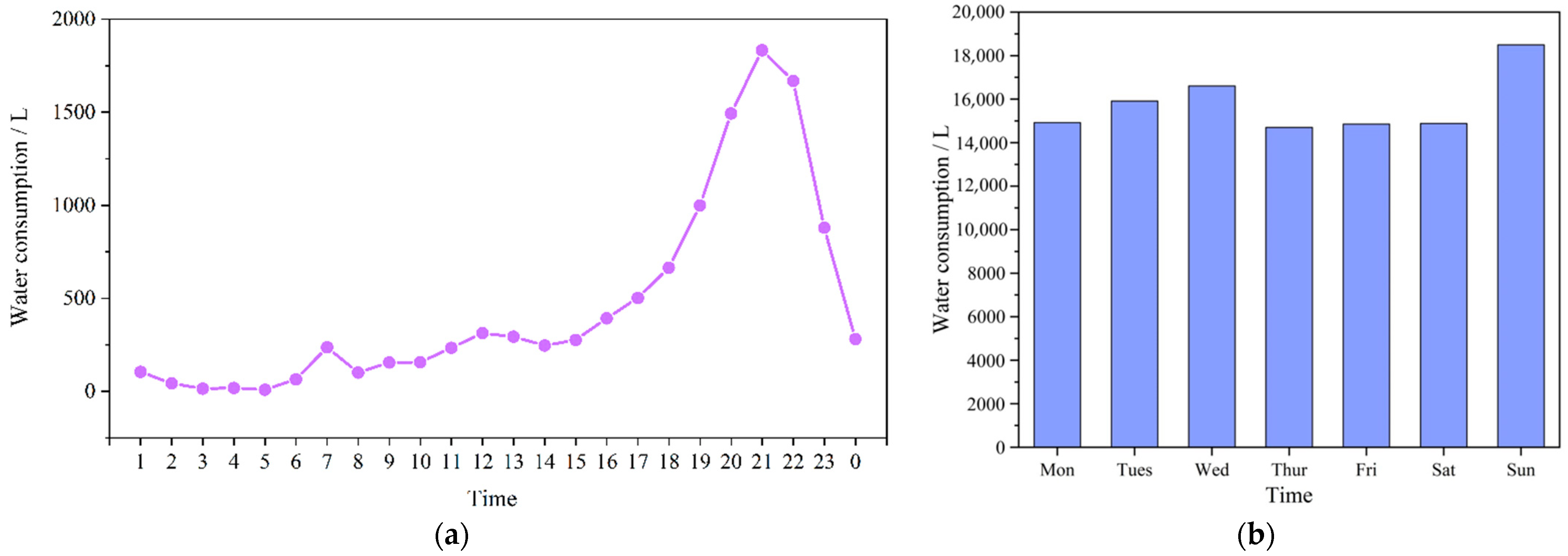
2.2. Analysis of Water Usage Habits

Through statistics, the daily DHW consumption in this period was determined. The collected data were analyzed to obtain the variation characteristics of water consumption in the student apartment. As shown in Figure 1, the water consumption of DHW was affected by seasonal factors. There was a disparity in consumption during winter and summer, with winter seeing high consumption levels and summer experiencing low levels. This was mainly because in the winter, due to the lower outdoor temperature, people feel cold and are more inclined to use hot water baths to keep warm. Summer temperatures are higher, and people may be more inclined to use cold water to bathe or reduce the use of hot water. The maximum water consumption is 30,408 L, the minimum is 3187 L, and the average is 15,768 L. The water consumption of DHW was also affected by personal habits. As shown in Figure 2a, this is the average daily hourly water consumption during data collection. There were three peaks in the average hourly water consumption: from 6:00 to 8:00, from 11:00 to 14:00, and from 18:00 to 0:00, with the highest water consumption in the evening. Everyone has different water habits. Some people like to shower in the morning to refresh their minds. Some people like to shower in the afternoon to keep their bodies refreshed, but the evening is the most frequent time to use water. Apart from variations across different time periods, the daily water usage also exhibited variations among different days of the week. As shown in Figure 2b, it is the average water consumption spent in one day from Monday through Sunday during the data collection period. It can be seen that Sunday was the period with the highest use of hot water for bathing. This may have been because there is usually more time for bathing and relaxation on this rest day. In summary, the water consumption of DHW showed certain variation characteristics in different seasons and periods. These variations are influenced by many factors, such as seasonal factors, personal habits, and rest days.

3. Methodology

By using big data and artificial intelligence technology, the accurate prediction of DHW consumption can be realized, which provides support for the water supply system. By collecting a large amount of historical water data and combining deep learning algorithms, a water model can be established to predict water consumption for a period in the future. This prediction can supply an exact message for the operators of the water supply system so that they can reasonably arrange the water supply plan, optimize the production scheduling, and improve the efficiency of the water supply system. By analyzing big data, we can understand the trends and variations in DHW use and identify water use patterns in different periods and different weather conditions. At the same time, artificial intelligence technology can automatically learn and adjust water models so that they can adapt to changing environmental conditions and user behaviors. By continuously collecting real-time water data and updating the model, the system has the potential to enhance prediction precision continuously, thereby offering more precise recommendations for water supply planning and scheduling. Using big data and artificial intelligence to accurately predict the water usage of DHW can not only improve the efficiency and management level of the water supply system but can also reduce the occurrence of an excess or insufficient water supply, conserve water resources, and reduce the operating costs of the water supply system. Therefore, the application of big data and artificial intelligence technology will bring many benefits to the operation and scheduling of the water supply system and promote the water supply industry to move in the direction of intelligent and sustainable development.

3.1. Artificial Neural Network

An ANN is a multi-layer feedforward network based on error backpropagation training of the parameters. It is generally composed of an input layer, an output layer, and a hidden layer [29]. As shown in Figure 3, the operation of an ANN essentially entails two primary procedures: a forward propagation of the working signal and a backward propagation of the error. During forward propagation, the ANN allots weights and biases to the input of each layer and computes its output, which serves as the input for the succeeding layer. Every neuron in the ANN is designated a particular weight, and a transfer function is employed to compute the weighted sum of the input and bias. After the transfer function calculates the sum, the activation function obtains the result until it receives the output so that it can trigger the appropriate result from the node.

In the prediction problem, an ANN can make predictions by learning the mapping relationship from input to output. Through the combination of multiple hidden layers and nodes, an ANN can learn more complex features and patterns to improve the accuracy of the prediction. In the typical training procedure of an ANN, the gradient descent approach is commonly utilized to revise the connection weights among nodes, with the objective of minimizing the disparity between the predicted output and the genuine value [30]. The specific formulas are as follows:

$$y=f(w{x}_i+b)$$

(1)

where x_i is the input value at the current moment; y is the output value; w and b are the weight value and the deviation value respectively; and f is the transfer function.

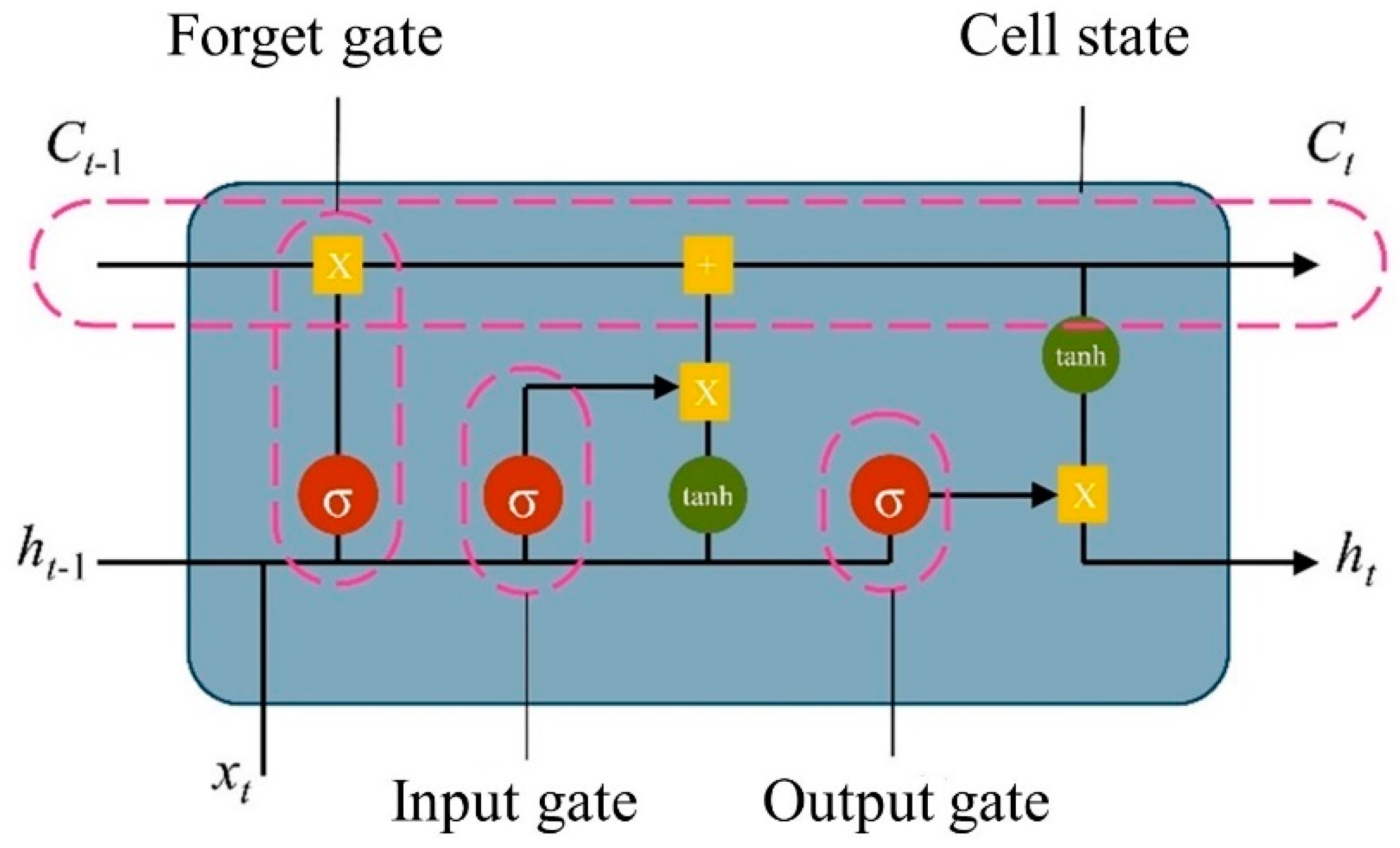
3.2. Long Short-Term Memory

Recurrent neural networks exhibit short-term memory, gradient explosion, gradient disappearance problems, and long-term time dependence. Hochreiter et al. [31] developed the LSTM model to overcome gradient disappearance problems. The LSTM model realizes the modeling of long-term dependencies by introducing three gates to control the input, output, and forgetting of information. As shown in Figure 4, these three gates are the input gate, forget gate, and output gate.

In the LSTM model, the input gate passes the message retained in the previous layer and the new message of the current input to two activation functions. The sigmoid function mainly fuses the current input signal with the output state of the previous moment to obtain a weight vector with a value range of [0, 1], while the tanh function mainly establishes a new candidate value vector. Both represent the importance of the current input signal to the internal state. The weight vector can be used to filter irrelevant input signals, retain only the most useful information, and finally multiply the output values of the two activation functions. The specific formulas are as follows:

$$S(x)=\frac{1}{1+e^{-x}}$$

(2)

$$\tanh =\frac{e^x-e^{-x}}{e^e-e^{-x}}$$

(3)

$$i_t=\sigma (W_i\cdot [h_{t-1},x_i]+b_i)$$

(4)

$${\stackrel{-}{C}}_t=\tanh (W_c\cdot [h_{t-1},x_t]+b_c)$$

(5)

$$C_t=f_t\otimes C_{t-1}+i_t\otimes {\stackrel{-}{C}}_t$$

(6)

where i_t and $\stackrel{-}{C_t}$ are the outputs of the sigmoid and tanh functions, respectively; W_i and W_c represent the weight matrices of the two layers; b_i and b_c represent the bias vectors of the two layers; the subscript c corresponds to the output gate; and C_t is the cell state output to the next time unit.

The forget gate is mainly used to fuse the cell state C_t−1 of the previous moment with the input signal of the current moment through to obtain a weight vector with a value range of [0, 1], which can represent the forgetting ratio of each state value. Close to 0 represents forgetting, and close to 1 can be retained. This is represented as follows:

$$f_t=\sigma (W_f\cdot [h_{t-1},x_t]+b_f)$$

(7)

where x_t is the input value of the current time; h_t−1 is the output value of the upper hidden state; W_f and b_f are the weight matrix and bias vector of the layer, respectively; and the subscript f corresponds to the forget gate.

The output gate mainly determines the value of the next hidden state and fuses the input signal of the current moment with the output state of the previous moment through the activation function:

$$o_t=\sigma (W_o\cdot [h_{t-1},x_t]+b_o)$$

(8)

$$h_t=o_t\otimes \tanh (C_t)$$

(9)

where W_o and b_o denote the weight matrix and bias vector, respectively; h_t is the output value passed to the next hidden state; and the subscript o represents the output gate.

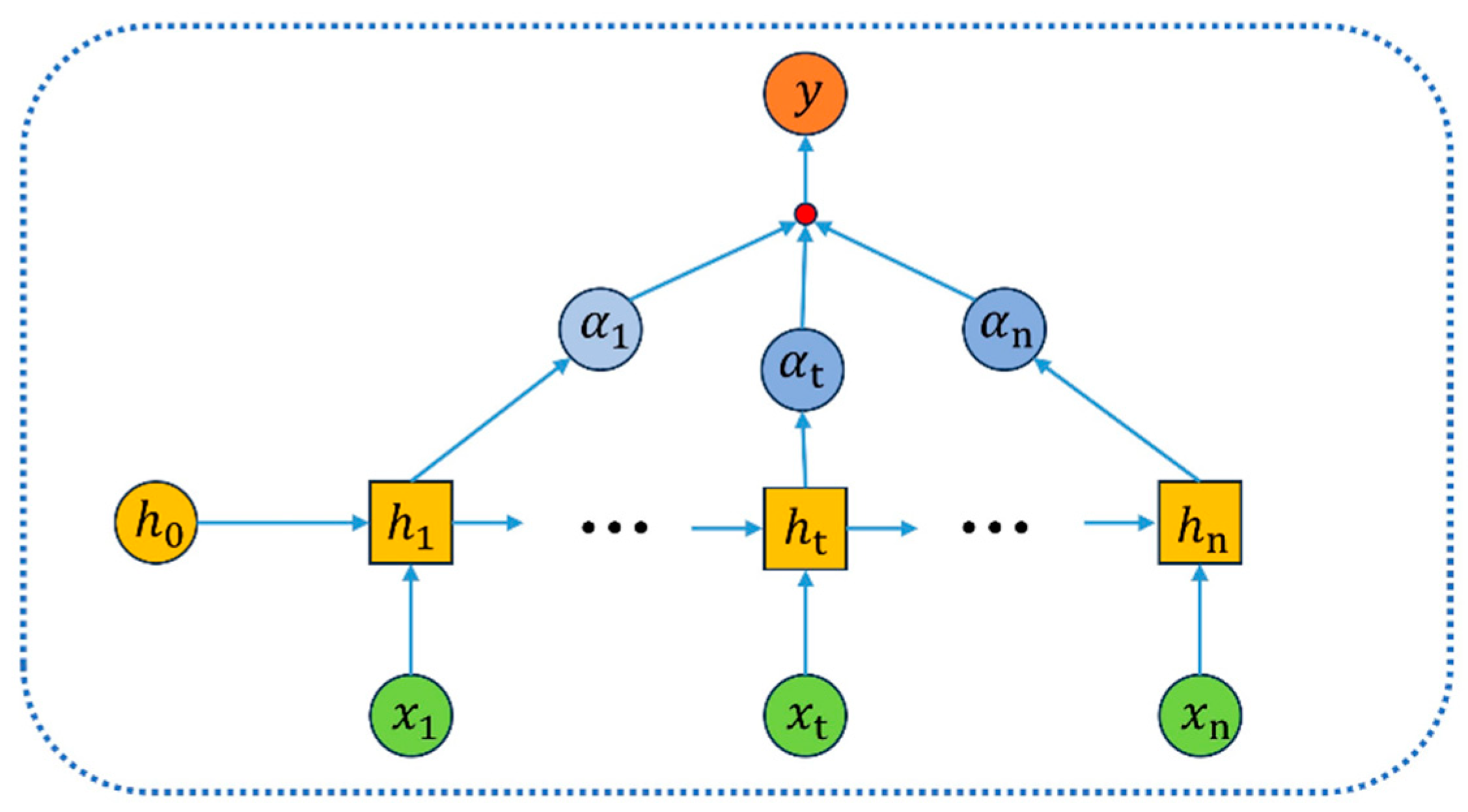
3.3. Attention Mechanism

The AM is a mechanism for allocating resources, as shown in Figure 5. This mechanism mimics human attention by focusing on related areas while reducing attention to unrelated areas. This mechanism enhances the importance of key information and ameliorates the veracity of the model by discarding unimportant information and amplifying key information [32]. The AM achieves this using a probability distribution to pay full attention to key information and compensates for the information loss created by the long sequence of the LSTM. The AM treats the importance of different features in each layer of the network as different, and the subsequent layers should pay more attention to the significant information and suppress the nonsignificant information. The introduction of an AM can improve the pattern discovery and representation ability of the model on sequence or ensemble data, thus ameliorating the prediction exactitude. The equations of the AM are as follows:

$$e_t=u\tanh (W{h}_t+b)$$

(10)

$${\alpha }_t=\frac{\exp (e_t)}{{\displaystyle \sum _{j=1}^t{e}_j}}$$

(11)

$$s_t={\displaystyle \sum _{t=1}^i{\alpha }_t{h}_t}$$

(12)

The attention scoring function e_t is responsible for calculating the correlation between the power load at time t and the LSTM network layer output vector. The weight coefficient is represented by u and W, and the output of the attention layer at time t is represented by S_t.

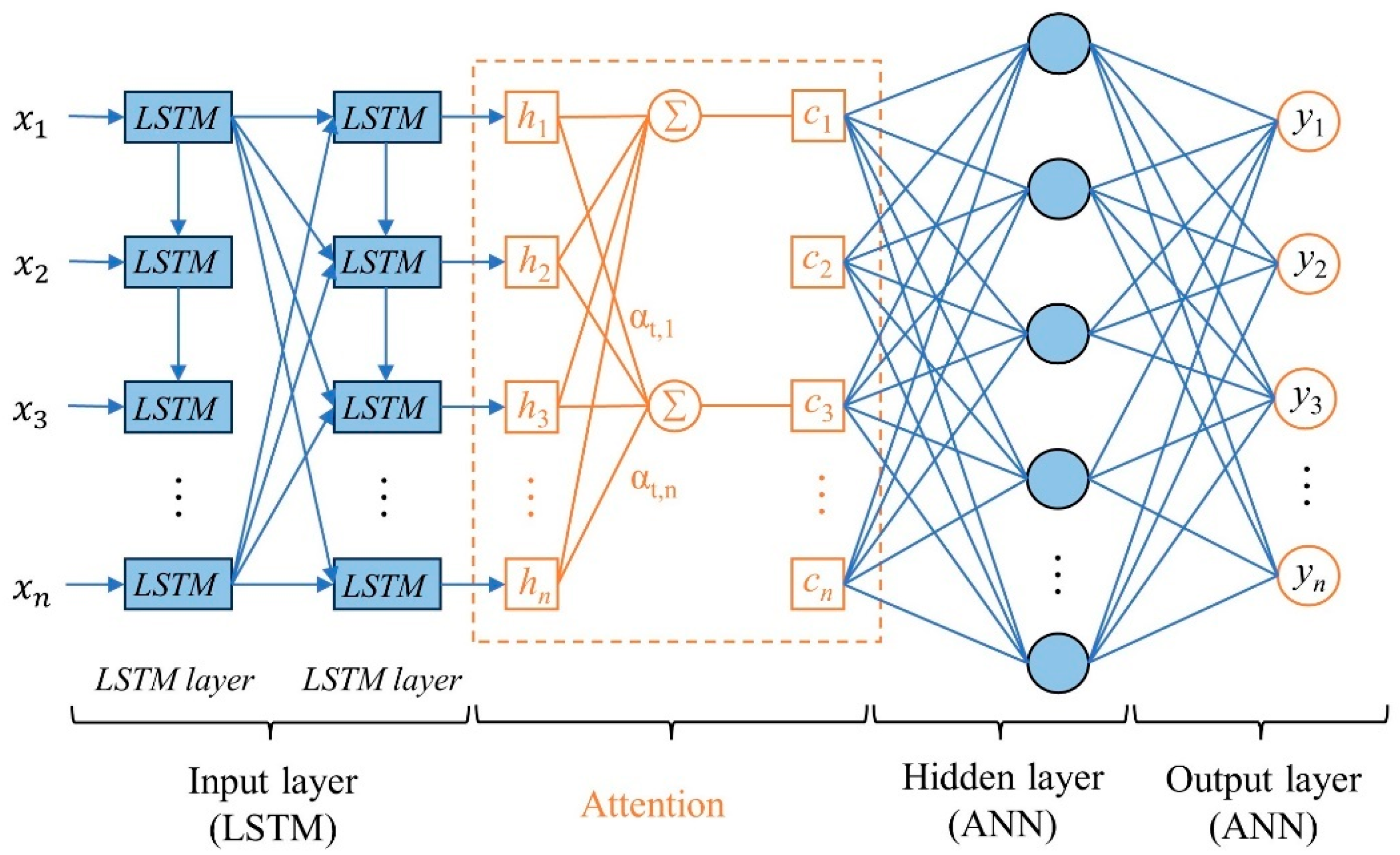
3.4. ANN-LSTM-A Model

Given the limitations of the ANN algorithm mentioned earlier in the prediction of water usage in the centralized hot water system of college student apartments, the ANN often fails to obtain the time dependence for time series data, resulting in inaccurate prediction results. To overcome this problem, this paper proposes an ANN-LSTM-A model. On account of the combination of the ANN and LSTM algorithms, the AM is introduced. While improving the ability to model sequence data, the AM can be fully used to advance the model’s pattern discovery and representation ability on sequence or ensemble data, thereby further improving the prediction exactitude of the entire model, as shown in Figure 6.

The features used to predict student water consumption were the date and water usage. The attributes were organized in a comma-separated value file (CSV) file and fed into the ANN-LSTM-A model, comprising an input layer, an AM layer, a hidden layer, and an output layer. The input layer employed the LSTM neural network due to its frequent application in sequence data analysis, with an inserted AM layer between the LSTM and the ultimate output layer. The hidden and output layers utilized ANNs. In the LSTM layer, the input was passed to the LSTM unit through the time step. The LSTM layer captured the time dependence of the input data and took the hidden state and the cell state as the outputs. The hidden state, which houses the sequence data, was cyclically forwarded to the succeeding time step. The hidden state of the last time step of the sequence was used as the context vector of the model. Next, the context vector was processed through the AM layer, and the important input data were weighted and fused. Then, the output of the LSTM layer weighted by the AM was mapped to the hidden layer (ANN). The AM layer was designed to learn and concentrate on the more significant time steps within the LSTM layer. Finally, the output from the active hidden layer was transferred to the output layer.

4. Prediction and Analysis

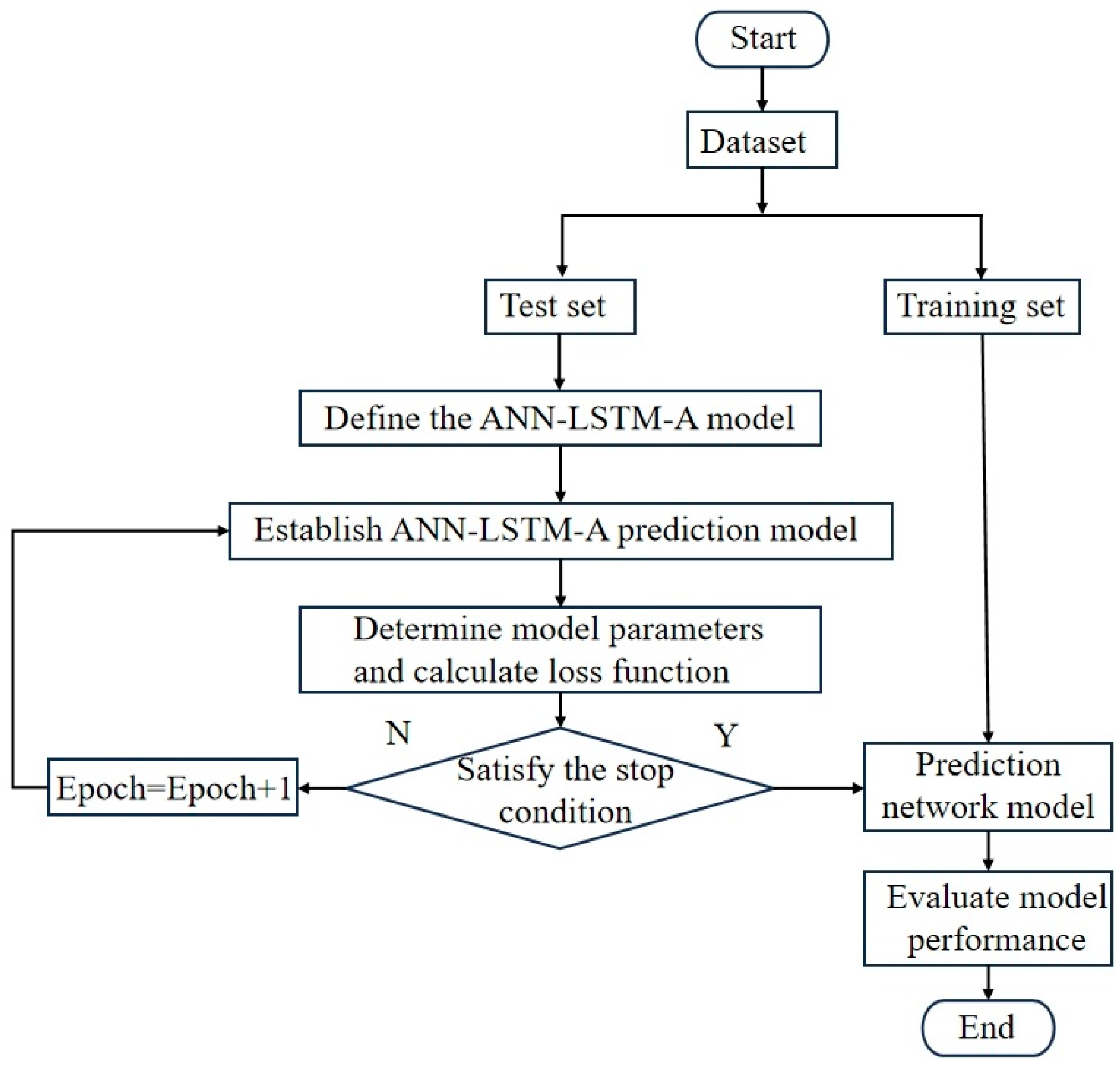
4.1. Experimental Process

The experimental process of the ANN-LSTM-A model for predicting DHW consumption in the student apartment is shown in Figure 7 and described as follows.

(1)

The DHW consumption data were normalized, 90% of the datasets were used for training, and the remaining 10% were used for testing.

$$X\prime =\frac{\left(X-X_{\min }\right)\times 2}{\left(X_{\max }-X_{\min }\right)-1}$$

(13)

where X is the raw input data of the network model, X_max and X_min are the maximum and minimum values of the raw data, respectively, and X′ is the value after normalization.

(2)

The input and output of the ANN-LSTM-A model were determined, and the ANN-LSTM-A-based model for predicting DHW consumption was developed with the goal of determining the optimal number of iterations, batch size, and other relevant hyperparameters.

(3)

The ANN-LSTM-A model was trained, and the weights and bias values were optimized according to the output error of each iteration.

(4)

When the number of training iterations reached the maximum number, the training ended, and the ANN-LSTM-A model began to predict DHW consumption. If the number of training iterations did not reach the maximum number, the process returned to (3) to continue the iterations.

(5)

The test dataset was used to test the determined ANN-LSTM-A model, and the corresponding root mean square error (RMSE) and mean absolute error (MAE) values were calculated.

Figure 7. Experimental flowchart of water consumption prediction.

Figure 7. Experimental flowchart of water consumption prediction.

4.2. Evaluation Indicators

To contrast with the performance of the model, RMSE and MAE were used to measure the exactitude of the prediction models. The RMSE is a metric used to evaluate the disparity between the predicted values of a model and the actual observed values. It calculates the square root of the average difference between the predicted values and the observed values. The purpose is to assess the prediction accuracy of the ANN-LSTM-A model on the test dataset. A lower RMSE value indicates a smaller variance between the model’s predictions and the actual observed values, implying a higher accuracy of the model. The MAE is another commonly employed metric to measure the dissimilarity between the predicted values of a model and the actual observed values. It calculates the mean absolute difference between the predicted values and the actual observed values. A lower MAE value signifies a smaller average absolute difference between the model’s predictions and the actual observed values, indicating a higher accuracy of the model. The formulas are as follows:

$$\mathit{RMSE}=\sqrt{\frac{1}{n}\sum _{i=1}^n{\left({\hat{y}}_i-y_i\right)}^2}$$

(14)

$$MAE=\frac{1}{n}\sum _{i=1}^n\left|{\widehat{y}}_i-y_i\right|$$

(15)

where ${\widehat{y}}_i$ is the predicted value, $y_i$ is the actual value, ${\overline{y}}_i$ is the average value, and n is the total number of samples.

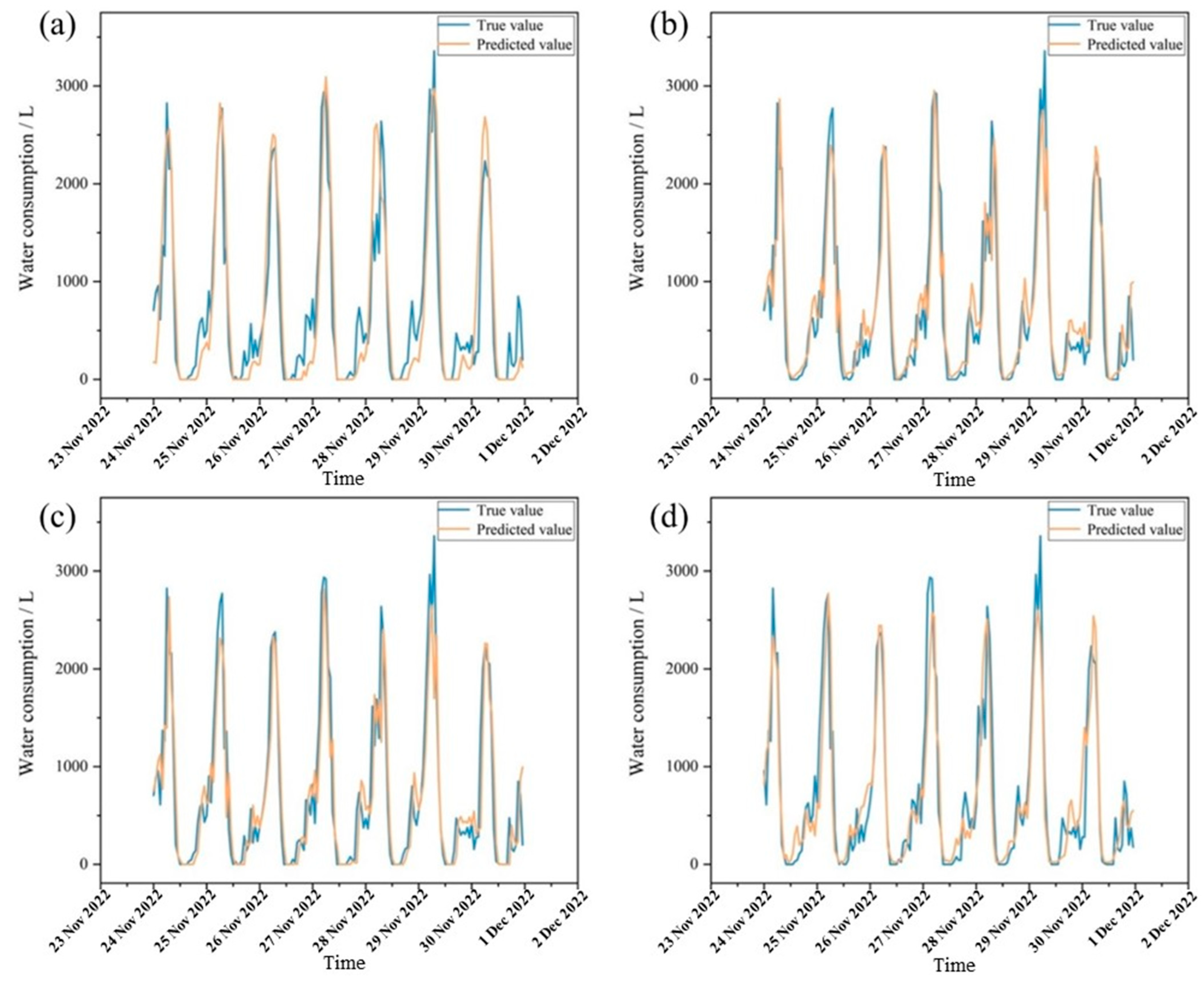
4.3. Comparison of Multi-Model Prediction Results

Nine months of water consumption data were used for statistics to facilitate the comprehensive capture of the long-term trend and periodicity of water consumption. By analyzing long-term data, seasonal fluctuations and long-term trends could be revealed. In the training of a deep learning model, selecting short-term daily and weekly data as prediction samples yields predictions in these timeframes, which can better reflect the current situation and trend of water consumption. In addition, short-term data are more easily learned and understood by deep learning models, and more accurate prediction models are trained. Therefore, based on the given historical water consumption data, we used four different deep learning models, ANN, LSTM, ANN-LSTM, and ANN-LSTM-A, to predict the water consumption on 30 November 2022, and from 24 November to 30 November 2022.

As shown in Figure 8, the forecasting outcomes of the ANN-LSTM-A model closely aligned with the actual values. Each model yielded different accuracies and deviations in the same period. Figure 9a shows the comparison between the water consumption prediction results of the ANN model and the actual values. It can be observed from the graph that there was a certain level of deviation between the predicted values and the actual values of the ANN model. The RMSE and MAE values were 0.39 and 0.27, respectively. Figure 9b illustrates the comparison between the predictions of the LSTM model and the actual values for water consumption. The LSTM model showed better accuracy and smaller deviations in its predictions than the ANN model, with RMSE and MAE values of 0.38 and 0.26, respectively. Figure 9c shows the comparison between the water consumption prediction results of the ANN-LSTM model and the actual value. Compared with the ANN and LSTM models, the prediction accuracy and deviation of the ANN-LSTM model were improved, and the RMSE and MAE values were 0.38 and 0.25, respectively. Figure 9d shows the water consumption prediction results of the ANN-LSTM-A model compared to the actual values. Notably, the predictions of the ANN-LSTM-A model exhibited greater proximity to the actual values compared to the other three models. The model demonstrated promising performance with RMSE and MAE values of 0.33 and 0.23, respectively.

Table 1. Performance evaluation of different prediction models.

Model	RMSE	MAE
ANN	0.39	0.28
LSTM	0.38	0.26
ANN-LSTM	0.38	0.25
ANN-LSTM-A	0.33	0.23

shows the performance evaluations of diverse prediction models. The RMSE and MAE values of the ANN-LSTM-A model were 15.4% and 17.9% lower than those of the ANN model, respectively. Similarly, the RMSE and MAE values of the ANN-LSTM-A were, respectively, 13.2% and 11.5% lower than those of the LSTM model. The RMSE and MAE were, respectively, 13.2% and 8% lower than those of the ANN-LSTM model. As shown in Figure 10, the RMSE and MAE of the ANN-LSTM-A were smaller than those of the other prediction models. By comparing the ANN-LSTM and ANN-LSTM-A models, it was found that the introduction of the AM had significant advantages in the DHW consumption prediction. The addition of AM in the model facilitated dynamic learning and an adjustment of weights at various time points. This feature enabled the model to selectively emphasize and highlight crucial features within the input data. After introducing the AM, the ANN-LSTM-A model could adaptively adjust the weights to better acquire the important dependencies in the data.

In summary, by observing and comparing the prediction results of four deep learning models, we found that each model may show different accuracies and deviations in the same period. Among the four models, the ANN-LSTM-A model had the first-rate prediction results, which were close to the actual water consumption values. This shows that when processing sequence data, the introduction of the LSTM network could effectively mine the information in the historical data. Simultaneously, the combination of the ANN and LSTM enabled the model to acquire the long-term dependencies of the time series data while learning the high-order features of the data. When the AM was appended, the model could automatically learn key information with a higher accuracy and further improve the prediction effect. Therefore, through comparative analysis, the ANN-LSTM-A model, which combined an ANN, an LSTM, and an AM, exhibited a more accurate prediction ability in predicting water consumption.

Kupiec’s p-test is a statistical test commonly used to evaluate the accuracy of risk models. Its main purpose is to test the accuracy of the Value at Risk (VaR) model, which predicts a certain value that extreme market losses will not exceed. The p-value of Kupiec is used to evaluate the performance of the predictive model in tail events by calculating the p-value of Kupiec’s LR statistic. The p-value represents the probability corresponding to the Kupiec’s LR statistic calculated based on the empirical distribution function, which is used to determine the significance of the tail prediction accuracy of the prediction model. Although Kupiec testing is commonly used for VaR models, in principle, similar types of tail risk testing can be performed on any decision or predictive model. When applied to the DHW water consumption prediction model, a threshold is defined, and events above or below this threshold are considered extreme tail events. Here, the highest and lowest 10% water consumption were selected. Then, the accuracy of the model’s prediction of tail performance was evaluated by assessing the performance of the predicted and actual values at this extreme event threshold. A smaller p-value indicates that the predictive model performs more accurately in tail events. After the calculation, the p-value of the ANN-LSTM-A model was less than 0.01. If the p-value of the ANN-LSTM-A model was less than 0.01, it indicated that certain parameters or effects of the model had a highly significant impact on the output results at a statistical significance level of 0.01.

4.4. Learning Rate

To select the optimal learning rate, a series of tests were conducted, and different learning rates were compared using the same training parameters. As shown in Figure 11, four different learning rates were set for testing, and different loss function results were obtained. The four different learning rates were Lr = 0.1, 0.05, 0.01, and 0.001. First, Lr = 0.1 was used for training. The model exhibited rapid convergence, with the loss function value gradually decreasing throughout the training process. However, after reaching a certain point in training, the value of the loss function started to fluctuate, which may have been due to the large learning rate causing the model to jump too far in the parameter space and being unable to find the global optimal solution. In contrast, when Lr = 0.1, the loss function value in the training process decreased slowly, which could better balance the convergence speed and model performance. Then, Lr = 0.01 was used for training. In contrast to the results with larger learning rates, the loss function value of the model decreased more slowly during the training process, which indicated that Lr = 0.01 could converge more stably and achieve relatively good results in terms of the model performance. Finally, when using Lr = 0.001 for training, the loss function value in the model training process decreased very slowly, but the model’s performance on the test set did not show significant improvement. This shows that Lr = 0.001 was too small, which made the model unable to fully learn and adjust the parameters, and this shows that the convergence speed was too slow. Based on the above experimental results, Lr = 0.01 was the better choice. With Lr = 0.01, the training process could converge more stably, and the model achieved relatively good performance results.

5. Results and Discussion

Of the four different deep learning models, i.e., ANN, LSTM, ANN-LSTM, and ANN-LSTM-A, the ANN-LSTM-A model had the first-rate prediction effect. By using the ANN-LSTM-A model for predictions, the water consumption for the month from 1 November to 30 November 2022 was successfully predicted. As shown in Figure 12, from the observed results, it is evident that the model accurately captured the trend and fluctuations in water consumption. In the figure, the specific time series prediction values are compared with the actual values at the same period. The evaluation of the ANN-LSTM-A model reveals a strong fit to the actual data and consistent accuracy in most prediction instances. The results demonstrate that the model effectively predicts DHW consumption with a high level of accuracy.

The ANN-LSTM-A model combines the ANN algorithm and LSTM algorithm, and introduces an AM to better acquire the long-term dependencies of time series data. In the experiment, the model showed a higher accuracy in predicting DHW water consumption than using ANN, LSTM, and ANN-LSTM models alone. The performance of a model largely depends on the quality of data and preprocessing methods. Therefore, in practical applications, it is necessary to ensure that there is sufficient high-quality historical water use data to train the model, and to improve model performance through specific preprocessing steps such as feature normalization, denoising, and handling missing values. Furthermore, it is reasonable to use longer time series to analyze long-term trends and periodicity.

Although the ANN-LSTM-A model demonstrates promising results, there are several challenges that need to be addressed before it can be effectively applied in practice. One of the challenges is the influence of various factors on DHW water consumption, including seasonal resident habits, economic activities, and unforeseen events. The complexity introduced by these external factors requires further exploration in future studies to enhance the robustness and applicability of the model. Additionally, future research should incorporate more variables related to DHW water consumption, such as meteorological conditions, to develop a comprehensive forecasting framework. This approach would enable the model to provide accurate predictions in diverse environmental conditions, thus increasing its practical utility.

In conclusion, this study underscores the substantial potential of the ANN-LSTM-A model for improving the accuracy of DHW water consumption predictions and offers a new avenue for research aimed at enhancing energy efficiency. However, it is crucial to address these challenges and refine the model to realize its promise in optimizing energy management systems and achieving long-term energy savings and emission reductions.

6. Conclusions

In this study, an ANN-LSTM-A model was proposed, which included an input layer, an AM layer, a hidden layer, and an output layer. Based on the combination of the ANN and LSTM algorithms, an AM was introduced to address the issue of traditional ANN models struggling to capture long-term dependencies, such as lags and trends in time series, and to increase the exactitude of DHW consumption predictions. The main findings of this study were as follows.

(1)

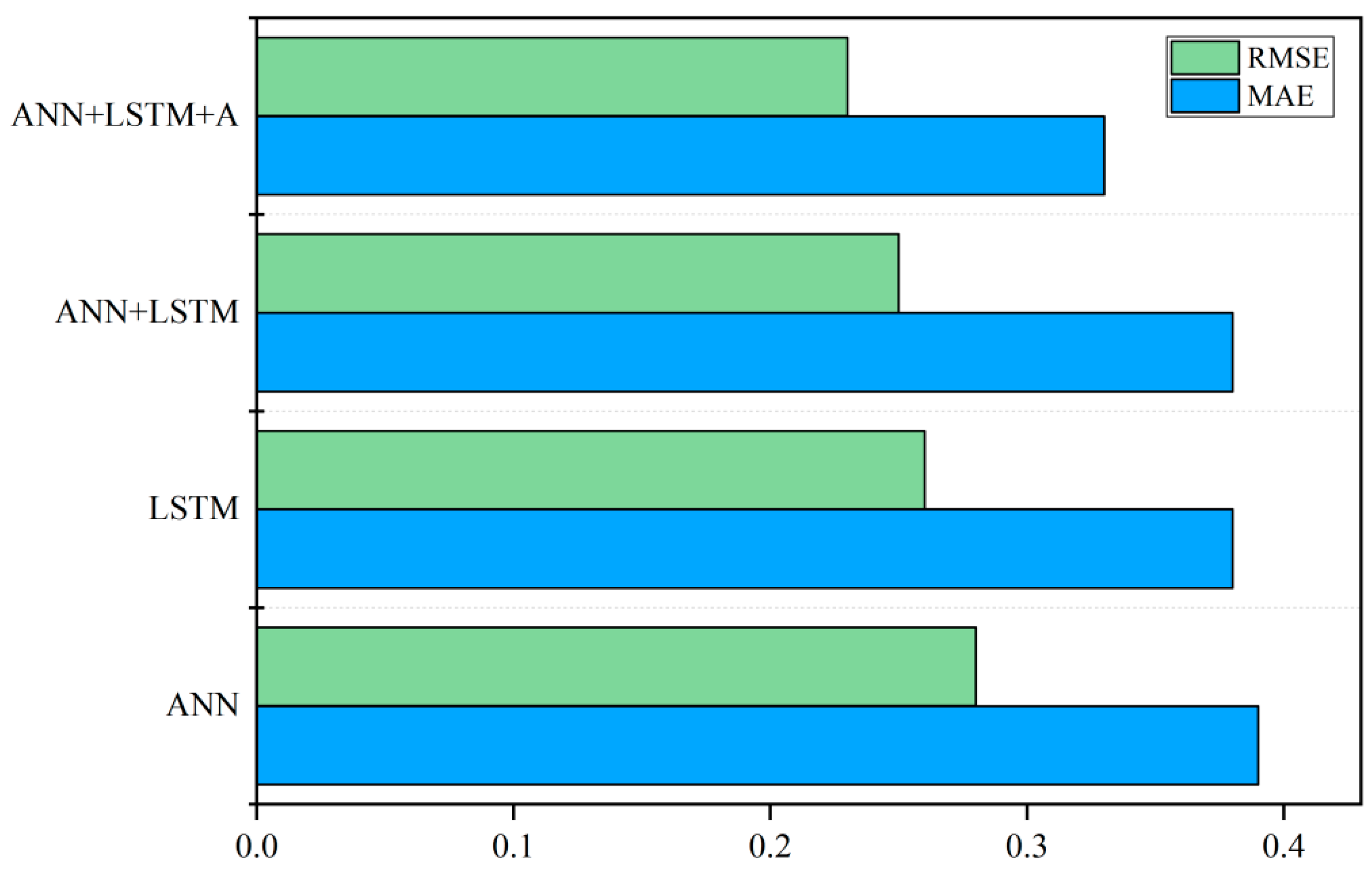
Upon comparing the prediction results of the ANN, LSTM, ANN-LSTM, and ANN-LSTM-A models, it was observed that the ANN-LSTM-A model yielded a significantly improved performance. The RMSE and MAE values achieved by the ANN-LSTM-A model were found to be 15.4% and 17.9% lower than those obtained by the ANN model, 13.2% and 11.5% lower than the LSTM model, and 13.2% and 8% lower than the ANN-LSTM model, respectively. These results indicate that the ANN-LSTM-A model showcased superior predictive capabilities and demonstrated a higher degree of accuracy in forecasting water consumption. The utilization of the ANN-LSTM-A model can hence be deemed advantageous in enhancing the accuracy of water consumption prediction.

(2)

By comparing the ANN-LSTM and ANN-LSTM-A models, it was found that the ANN-LSTM-A model with an AM could better capture the key information in the time series data and automatically learn the weights and importance of different time points to adapt to various changes and trends in different time series. This effectively improved the accuracy of the model in the prediction of DHW consumption, and thus, this model is a reliable prediction tool.

(3)

When predicting the DHW consumption of student apartments, various conditions will inevitably have a certain influence on the prediction accuracy. For instance, changes in weather have a significant impact on water consumption. Hence, to enhance the predictive accuracy of the model, it is essential to incorporate meteorological conditions, seasons, and other related factors. Further analysis and exploration of these factors in future studies will help improve the accuracy of water consumption prediction.

The findings indicate that the ANN-LSTM-A model is capable of delivering more precise and dependable predictions of DHW consumption. This carries significant implications for optimizing the design and operation of heating systems, enhancing energy efficiency, reducing energy consumption and carbon emissions, and advancing the objectives of energy conservation and emission reduction. In summary, the proposed ANN-LSTM-A model holds substantial potential for refining the accuracy of DHW consumption predictions. When compared to traditional deep learning models, particularly the LSTM model, the ANN-LSTM-A model demonstrates a marked improvement in accuracy. The predictive capacity of the ANN-LSTM-A model stands to facilitate the optimized design and operation of heating systems, offering a scientific foundation for the rational planning of water utilization and resource allocation, and elevating the efficiency and management standards of water supply systems.

References

1. Lyu, Y.; Gao, H.; Yan, K.; Liu, Y.; Tian, J.; Chen, L.; Wan, M. Carbon peaking strategies for industrial parks: Model development and applications in China. Appl. Energy 2022, 322, 119442. [Google Scholar] [CrossRef]
2. Liang, G. Research on the Evaluation System and Practice of Green Schools in the United States. Constr. Sci. Technol. 2013, 12, 35–38. [Google Scholar]
3. Deng, L.; Chang, X.; Wang, P. Daily Water Demand Prediction Driven by Multi-source Data. Procedia Comput. Sci. 2022, 208, 128–135. [Google Scholar] [CrossRef]
4. Yue, J.; Yang, H.; Feng, H.; Han, S.; Zhou, C.; Fu, Y.; Guo, W.; Ma, X.; Qiao, H.; Yang, G. Hyperspectral-to-image transform and CNN transfer learning enhancing soybean LCC estimation. Comput. Electron. Agric. 2023, 211, 108011. [Google Scholar] [CrossRef]
5. Zhang, J.; Xin, X.; Shang, Y.; Wang, Y.; Zhang, L. Nonstationary significant wave height forecasting with a hybrid VMD-CNN model. Ocean Eng. 2023, 285, 115338. [Google Scholar] [CrossRef]
6. Jing, Y.; Zhang, L.; Hao, W.; Huang, L. Numerical study of a CNN-based model for regional wave prediction. Ocean Eng. 2022, 255, 111400. [Google Scholar] [CrossRef]
7. Cinar, Y.G.; Mirisaee, H.; Goswami, P.; Gaussier, E.; Aït-Bachir, A. Period-aware content attention RNNs for time series forecasting with missing values. Neurocomputing 2018, 312, 177–186. [Google Scholar] [CrossRef]
8. Amalou, I.; Mouhni, N.; Abdali, A. Multivariate time series prediction by RNN architectures for energy consumption forecasting. Energy Rep. 2022, 8, 1084–1091. [Google Scholar] [CrossRef]
9. Wang, Y.; Li, T.; Lu, W.; Cao, Q. Attention-inspired RNN Encoder-Decoder for Sensory Time Series Forecasting. Procedia Comput. Sci. 2022, 209, 103–111. [Google Scholar] [CrossRef]
10. Chung, W.H.; Gu, Y.H.; Yoo, S.J. District heater load forecasting based on machine learning and parallel CNN-LSTM attention. Energy 2022, 246, 123350. [Google Scholar] [CrossRef]
11. Yao, J.; Wu, W. Wave height forecast method with multi-step training set extension LSTM neural network. Ocean Eng. 2022, 263, 112432. [Google Scholar] [CrossRef]
12. Fazlipour, Z.; Mashhour, E.; Joorabian, M. A deep model for short-term load forecasting applying a stacked autoencoder based on LSTM supported by a multi-stage attention mechanism. Appl. Energy 2022, 327, 120063. [Google Scholar] [CrossRef]
13. Huang, R.; Ma, L.; He, J.; Chu, X. T-GAN: A deep learning framework for prediction of temporal complex networks with adaptive graph convolution and attention mechanism. Displays 2021, 68, 102023. [Google Scholar] [CrossRef]
14. Yilmaz, B.; Korn, R. Synthetic demand data generation for individual electricity consumers: Generative Adversarial Networks (GANs). Energy AI 2022, 9, 100161. [Google Scholar] [CrossRef]
15. Yuan, R.; Wang, B.; Mao, Z.; Watada, J. Multi-objective wind power scenario forecasting based on PG-GAN. Energy 2021, 226, 120379. [Google Scholar] [CrossRef]
16. Singh, S.; Bansal, P.; Hosen, M.; Bansal, S.K. Forecasting annual natural gas consumption in USA: Application of machine learning techniques-ANN and SVM. Resour. Policy 2023, 80, 103159. [Google Scholar] [CrossRef]
17. Ravikumar, K.S.; Chethan, Y.D.; Likith, C.; Chethan, S.P. Prediction of Wear Characteristics for Al-MnO2 Nanocomposites using Artificial Neural Network (ANN). In Materials Today: Proceedings; Elsevier: Amsterdam, The Netherlands, 2023. [Google Scholar]
18. Nguyen, T.H.; Tran, N.L.; Phan, V.T.; Nguyen, D.D. Prediction of shear capacity of RC beams strengthened with FRCM composite using hybrid ANN-PSO model. Case Stud. Constr. Mater. 2023, 18, e02183. [Google Scholar] [CrossRef]
19. Neudakhina, Y.; Trofimov, V. An ANN-based intelligent system for forecasting monthly electric energy consumption. In Proceedings of the 2021 3rd International Conference on Control Systems, Lipetsk, Russia, 10–12 November 2021. [Google Scholar]
20. Afandi, A.; Lusi, N.; Catrawedarma, I.; Subono; Rudiyanto, B. Prediction of temperature in 2 meters temperature probe survey in Blawan geothermal field using artificial neural network (ANN) method. Case Stud. Therm. Eng. 2022, 38, 102309. [Google Scholar] [CrossRef]
21. Rodrigues, F.; Cardeira, C.; Calado, J.M.F. The daily and hourly energy consumption and load forecasting using artificial neural network method: A case study using a set of 93 households in Portugal. Energy Procedia 2014, 62, 220–229. [Google Scholar] [CrossRef]
22. Bennett, C.; Stewart, R.A.; Beal, C.D. ANN-based residential water end-use demand forecasting model. Expert Syst. Appl. 2013, 40, 1014–1023. [Google Scholar] [CrossRef]
23. Walker, D.; Creaco, E.; Vamvakeridou-Lyroudia, L.; Farmani, R.; Kapelan, Z.; Savić, D. Forecasting domestic water consumption from smart meter readings using statistical methods and artificial neural networks. Procedia Eng. 2015, 119, 1419–1428. [Google Scholar] [CrossRef]
24. Pascanu, R.; Mikolov, T.; Bengio, Y. On the difficulty of training recurrent neural networks. In Proceedings of the 30th International Conference on Machine Learning, Atlanta, GA, USA, 16–21 June 2013. [Google Scholar]
25. Greff, K.; Srivastava, R.K.; Koutník, J.; Steunebrink, B.R.; Schmidhuber, J. LSTM: A search space odyssey. IEEE Trans. Neural Netw. Learn Syst. 2016, 28, 2222–2232. [Google Scholar] [CrossRef] [PubMed]
26. Sherstinsky, A. Fundamentals of recurrent neural network (RNN) and long short-term memory (LSTM) network. Phys. D 2020, 404, 132306. [Google Scholar] [CrossRef]
27. Niknam, A.; Zare, H.K.; Hosseininasab, H.; Mostafaeipour, A. Developing an LSTM model to forecast the monthly water consumption according to the effects of the climatic factors in Yazd, Iran. J. Eng. Res. 2023, 11, 100028. [Google Scholar] [CrossRef]
28. Heidari, A.; Khovalyg, D. Short-term energy use prediction of solar-assisted water heating system: Application case of combined attention-based LSTM and time-series decomposition. Sol. Energy 2020, 207, 626–639. [Google Scholar] [CrossRef]
29. Xu, Y.; Li, F.; Asgari, A. Prediction and optimization of heating and cooling loads in a residential building based on multi-layer perceptron neural network and different optimization algorithms. Energy 2022, 240, 122692. [Google Scholar] [CrossRef]
30. Vijayalakshmi, K.; Vijayakumar, K.; Nandhakumar, K. Prediction of virtual energy storage capacity of the air-conditioner using a stochastic gradient descent based artificial neural network. Electr. Power Syst. Res. 2022, 208, 107879. [Google Scholar] [CrossRef]
31. Hochreiter, S.; Schmidhuber, J. Long short-term memory. Neural Comput. 1997, 9, 1735–1780. [Google Scholar] [CrossRef]
32. Niu, Z.; Zhong, G.; Yu, H. A review on the attention mechanism of deep learning. Neurocomputing 2021, 452, 48–62. [Google Scholar] [CrossRef]
Figure 1. Daily variation in domestic hot water (DHW) water consumption.
Energies 17 01102 g001
Figure 2. (a) Average daily water consumption per hour during the data collection period; (b) average single-day water consumption from Monday to Sunday during data collection.
Energies 17 01102 g002
Figure 3. Artificial neural network (ANN) network structure.
Energies 17 01102 g003
Figure 4. Long short-term memory (LSTM) network structure.
Energies 17 01102 g004
Figure 5. Attention mechanism structure.
Energies 17 01102 g005
Figure 6. ANN-LSTM-A model.
Energies 17 01102 g006
Figure 8. Comparison of the actual and predicted values of 1-day water consumption for different models.
Energies 17 01102 g008
Figure 9. (a) Comparison between the actual and predicted values of the 7-day water consumption for ANN models; (b) Comparison between the actual and predicted values of the 7-day water consumption for LSTM models; (c) Comparison between the actual and predicted values of the 7-day water consumption for ANN-LSTM models; (d) Comparison between the actual and predicted values of the 7-day water consumption for ANN-LSTM-A models.
Energies 17 01102 g009
Figure 10. Comparison of error evaluation indices of different models.
Energies 17 01102 g010
Figure 11. Loss function results at different learning rates.
Energies 17 01102 g011
Figure 12. Actual and predicted monthly water consumption of the ANN-LSTM-A model.
Energies 17 01102 g012