Abstract
A significant amount of energy in wastewater treatment plants is spent on aeration to treat the organic matter with microorganisms in an oxygen-enriched environment. In this study, a novel and simplistic aeration concept known as Confined Tube Aeration (CTA) is proposed, in which the main elements are a Venturi injector and a coiled tube at its outlet. Two Venturi injector diameters were chosen for evaluation in this study, measuring 1 inch (25.4 mm) and 4 inch (101.6 mm). In this study, a relationship was developed between air suction rate and pressure differential across the injector. Then, a numerical model was developed to analyze hydrodynamic conditions and evaluate system performance. The main findings are that the larger diameter aerator performs 20% better than the smaller injector in terms of standard aeration efficiency (SAE), with a maximal value of 0.74 kgO2/kWh found for the larger diameter system. These results suggest that future SAE improvements may be made for larger diameter systems in full-scale wastewater treatment applications with suitably designed injectors.
1. Introduction
Aeration is the process of bringing air and water into close contact to promote mass transfer of oxygen. Aeration is required for the proper growth of microorganisms in a wastewater treatment aeration basin for timely decomposition of organic materials. Aeration accounts for 30% to 75% of total energy consumption of wastewater treatment plants [1,2]. Oxygenation of water is accomplished using devices called aerators, whose primary purpose is to enhance mass transfer down a concentration gradient by increasing gas–liquid surface area. These aerators, which come in a variety of designs, are typically compared using two indicators: standard oxygen transfer rate (SOTR, in kgO2/h) and standard aeration efficiency (SAE, in kgO2/kWh).
There are generally two classes of aerators: surface aerators, which discharge water into the air, and diffused aerators, which release gaseous oxygen into the water column. The latter is by far the most common in industry due to higher SAE [3]. Here, blowers or compressors move ambient air through a network of pipes, terminating in porous pipes or disks arranged at the bottom of the basin [4]. Diffusers with fine pores are capable of producing microbubbles in the range of 10 μm to 60 μm [3] and are very efficient in diffusing gas to the liquid because of the large gas–liquid interfacial area, longer residence time, and hence higher mass transfer rates [5]. Such diffusers are generally categorized into fine and coarse bubble diffusers based on the bubble sizes produced [6]; fine-bubble diffusers produce smaller bubbles (2–5 mm in diameter) than coarse-bubble diffusers (6–10 mm) [7]. Since bubbles require residence time to transfer oxygen effectively, aeration tanks must be sufficiently (up to 10 m) deep to optimize oxygen transfer. Furthermore, a deep aeration tank provides higher hydrostatic pressure, which increases the local saturation of dissolved oxygen concentration, which, in turn, increases the oxygen deficit to promote increased mass transfer. However, diffused aeration has its own drawbacks. For starters, generating microbubbles requires a higher compression cost due to the significant pressure drop through the small pores. Diffuser systems can also easily be clogged and require higher upfront costs due to the complexity of installations [8]. However, their high mass transfer efficiency makes them nonetheless quite energy efficient and can achieve SAE values up to 4.56 kgO2/kWh [9] for fine pore diffusers, whereas coarse bubble diffusers enjoy SAE values typically in the 1.22–2.13 kgO2/kWh range.
Another type of diffused aerator is the Venturi aerator. Here, a submersible pump is located near the base of the aeration basin with a piping system where a Venturi device is attached and through which liquid is circulated. Venturi aerators can draw air from the surface naturally in a throat based on Bernoulli’s principle; therefore, no compressor is required. Venturi aerators generally consume less energy than conventional airlift reactors, bubble columns, and stirred tanks [3,10]. A Venturi bubble generator consists of a nozzle section, a suction chamber, and a divergent section [11]. Venturi aerators are capable of producing bubbles with a mean diameter below 100 m, thus providing high interfacial areas for mass transfer [12,13]. Additionally, the higher kinetic energy of liquid and gas flow creates intense turbulence and promotes mixing. Venturi aerators require higher liquid flow at the entrance of the injector to produce enough negative static pressure at the throat to entrain air and, therefore, can suffer from low efficiency. However, Venturi aeration systems are less energy intensive and less expensive to install and maintain as they have no moving parts that may break or fail. Moreover, they are less prone to clogging compared to coarse and fine bubble diffusers [14]. Venturi aerators generally have SAE values between 0.5 and 2.3 kgO2/kWh [15].
Several recent studies in the literature have been conducted to evaluate the performance of Venturi aerators for aquaculture and wastewater purposes. Yadav et al. [16] used a dimensionless technique to optimize performance of such an aeration system on the basis of Venturi geometric properties. Here, the maximal SAE was found to be 0.611 kgO2/kWh, and the nondimensional SAE was found to rely only on the (water) Reynolds number and Froude number. Dong et al. [17] analyzed commercially available injectors in series and parallel, with differing injection depths. It was found here that better aeration efficiency could be realized by connecting aerators in parallel, with a maximal SAE reported to be 0.306 kgO2/kWh. Zhu et al. [18] conducted a similar study and found that parallelizing injectors resulted in SAE values that doubled the series configuration (0.14 kgO2/kWh versus 0.07 kgO2/kWh). Dange and Warkhedkar [19] assessed the effectiveness of a Venturi aeration for the purposes of pond/river oxygenation on the basis of injector depth. It was found here that, within the injector depths investigated, deeper injection resulted in increased air flow rates in the system. The maximal reported SAE value was 0.2936 kgO2/kWh.
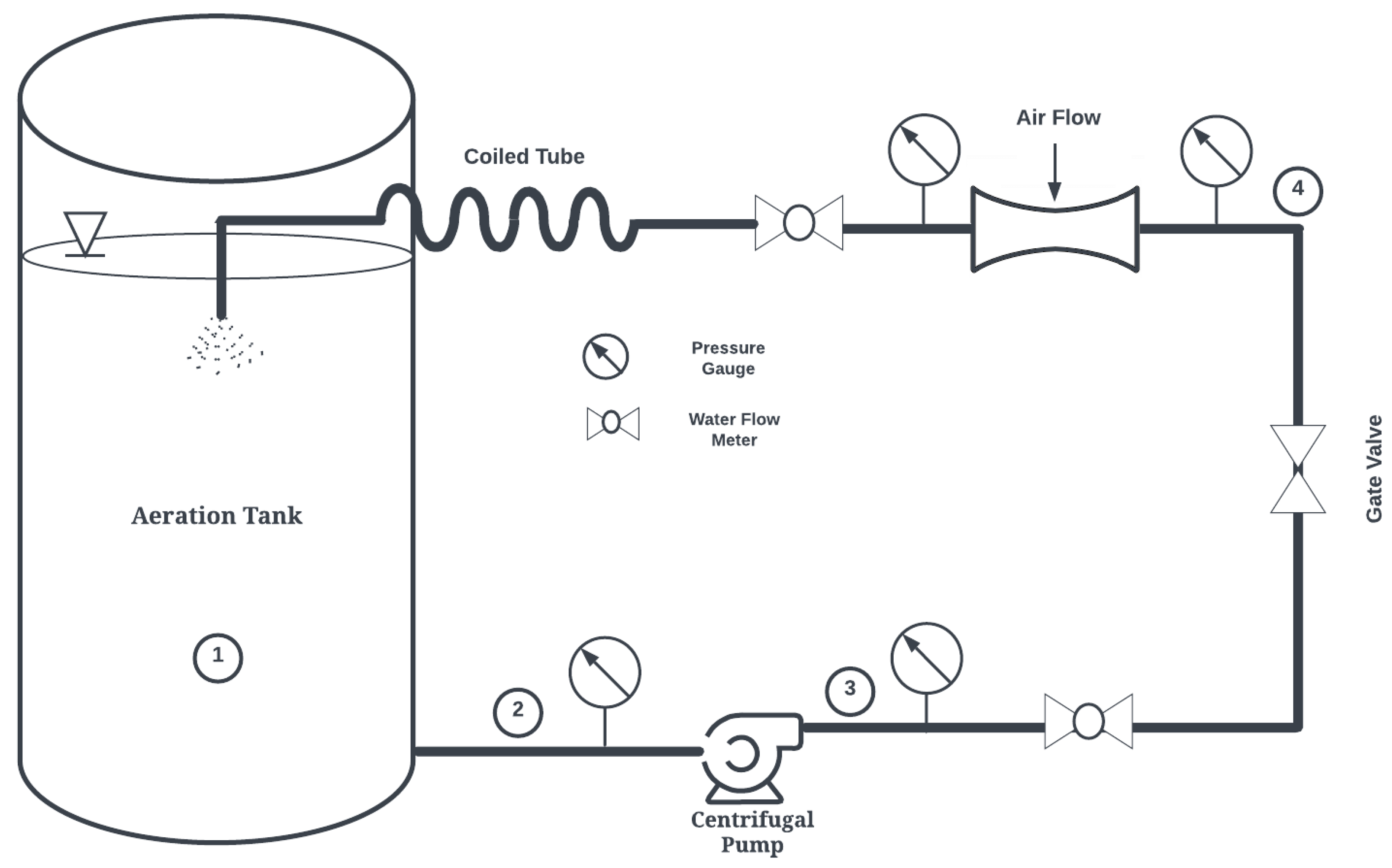
In this study, a novel Venturi bubble aeration system termed the Confined Tube Aerator (CTA) is proposed, previously introduced by the authors [20,21]. Figure 1 shows a schematic of the proposed system. The basic components of this aeration system are a pump, a Venturi injector, and a coiled tube. The pump draws water from the aeration basin and circulates it through the Venturi injector and coiled tube.
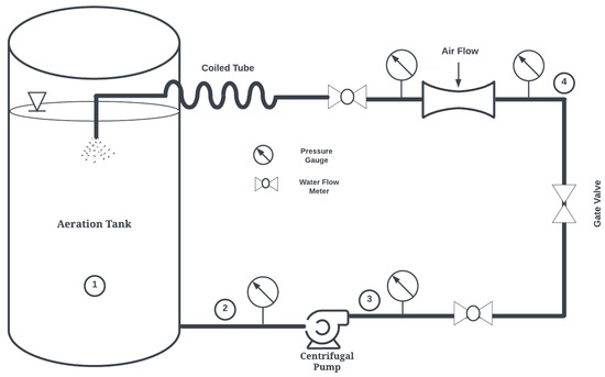
Figure 1.
Confined Tube Aerator (CTA) System Schematic. 1: Aeration tank. 2: Pump suction. 3: Pump discharge. 4: Venturi inlet. 5: Venturi discharge (CTA inlet).
With a horizontally oriented helical axis, the CTA may reduce bubble coalescence widely observed in horizontal pipes [22], maintaining a higher interfacial area necessary for increased oxygen transfer. This device has the potential to revolutionize wastewater treatment for several reasons:
- Pressure requirements are decreased as there is no need to discharge at the bottom of basins. CTA pumps may draw from the bottom of basins and discharge to the surface, enhancing mixing.
- Thermodynamic work is decreased since pumps are used in lieu of compressors or blowers. Membrane pressure losses experienced in bubble diffusers are also avoided.
- Maintenance costs, which can be substantial for bubble diffusers as they are prone to fouling from debris and dissolved surfactants [9], are decreased as VAs may be cleaned/replaced easily. Furthermore, the CTA system allows for placement of Venturi injectors on land, making replacement easier than if placed at the bottom of aeration basins.
- CTA systems do not require large, deep basins and may drastically reduce construction costs. They may also be particularly well suited for water treatment in remote settings and for oceanic vessels, where traditional aeration techniques are not feasible.
Furthermore, they are a potentially disruptive technology in the aquaculture aeration industry, as the current industry standard paddle wheel is of comparably low efficiency. The frequent use of dredge nets for fish harvesting make the use of bubble diffusers impractical.
In the current study, the performance of the proposed system is analyzed with respect to differing aerator sizes at varying hydrodynamic conditions. The discrete bubble model concept is used to model the mass transfer from bubbles to water in the tube, with the goal of improving aeration efficiency through parametric analysis of the results. This is the first study to estimate performance of CTA systems using commercially available Venturi injectors larger than 2.54 cm in diameter.
2. Methodology
The following is divided into five sections. The first discusses calculation of two-phase pressure drop in the coiled tube, the second explains aeration theory and performance parameters, the third outlines the theory underlying aeration prediction, the fourth discusses model validation with experiments, and the fifth gives an overview of the simulation procedure.
2.1. Two-Phase Pressure Drop
Flow inside the CTA tube is two-phase by nature. Accurate prediction of the two-phase flow pressure drop is important in designing and optimizing the CTA system’s performance. The total pressure loss gradient for a steady two-phase flow consists of three components—frictional pressure drop (), acceleration (momentum) pressure drop (), and gravitational pressure drop () [23]. Therefore, the total pressure drop is derived from the following equation:
In the above, and are ignored since the flow velocity of the two phases (air bubbles and water) is relatively constant along the length of the pipe and there are no changes in gravitational potential energy between the inlet and outlet. For simplicity, it is common to treat the two-phase mixture as a single phase with average properties of the two phases considering the homogeneously mixed flow assumption. However, a more accurate prediction can be made using a friction multiplier method [24]. Here, the frictional pressure drop in a pipe with two-phase flow can be described by the Darcy–Weisbach equation, as shown below:
where is a two-phase flow multiplier that accounts for the additional pressure losses due to the presence of both liquid and gas phases. The liquid-only frictional pressure drop, , is calculated using the following relation:
The two-phase flow multiplier, , is further defined as
with , and given by
here, , , and are the density, viscosity, and surface tension of the liquid. The subscripts l, g, and m represent the liquid phase, gas phase, and mixture, respectively. and are the Darcy–Weisbach friction factors for the liquid and gas phases, respectively, and is the gas quality:
The mixture’s Froude number () and Weber number () for the combined flow are calculated as follows:
In the above relationship, L, , and represent the length, diameter, and cross-sectional area of the pipe, respectively. The mixture density () is calculated as volume-weighted average of the gas () and liquid () densities as follows:
here, is the volume fraction of gas and is calculated as the ratio of the volumetric flow rate of the gas phase to the total volume flow rate of liquid () and gas phase ().
The Colebrook–White equation is used for friction factor calculation in turbulent flow [25], as there are no instances of laminar flow in this study:
here, e is the relative roughness, defined as the pipe diameter divided by tubing roughness (0.0015 mm for standard PVC piping utilized in this study). Additionally, since the CTA assembly is designed in this study to discharge at the surface of the water, the (gauge) pressure of the Venturi discharge in Figure 1 becomes the total pressure differential () in Equation (1).
2.2. Aeration Theory
The following equation describes the rate of oxygen transfer in an aeration system [26].
The left-hand side of the above represents the rate of change in the dissolved oxygen concentration in the liquid phase over time. Here, refers to the saturation concentration of the gas (O2 or N2) in the liquid, and represents the actual concentration at any given moment. is the overall mass transfer coefficient, which is a product of the liquid-phase mass transfer coefficient () and the specific interfacial area (). In practice, it is impractical to measure the interfacial area; as a result, the value of is measured.
Upon integration of Equation (14), considering initial concentration of at time and at any subsequent time , the following integrated form is derived:
This integral form allows experimental determination of by measuring over time. As approaches , the transfer rate diminishes, representing a near equilibrium state. Plotting the left-hand side of Equation (15) with respect to time helps determine from the slope.
is often normalized to a standard temperature of 20 °C, , to ensure consistency and comparability between different aeration system performances. The following standardized equation is used, where is the temperature correction factor (1.024 for pure water), and T is the water temperature during the experiment (°C) [27]:
The Standard Oxygen Transfer Rate (SOTR) is defined as the mass of oxygen transferred per unit of time into a fixed volume of water at standard conditions of 20 °C and 1 atm [28].
where denotes the saturation concentration of dissolved oxygen at 20 °C, V is the volume of water aerated, and the dimension of SOTR is kgO2/h. To quantify the efficiency of an aeration system, the Standard Aeration Efficiency (SAE) is often used, which has dimensions kgO2/kWh:
The power input can be either delivered power (DP) or wired power (WP) in the above equation.
2.3. Discrete Bubble Model (DBM)
In this study, a discrete bubble model (DBM) method was adopted to predict mass transfer inside the confined tube. This model is based on the one-dimensional time-dependent motion of spherical gas bubbles in the coiled pipe system. In this analysis, the effects of turbulence and agglomeration/breakup of bubbles are neglected, and the overall methodology is based on that found in [29]. The mass transfer flux () of a gas species across the surface of a single bubble is then written as follows:
where is the mass transfer coefficient, is the saturation concentration of the gas i in the liquid at the gas–liquid interface, and is the concentration of the gas i at the bulk liquid. Applying Henry’s law at the gas–liquid interface, the equilibrium concentration becomes
where is Henry’s constant, and is the partial pressure of gas i. The bulk aqueous-phase concentration of the gas i at liquid can be derived from the ideal gas law:
here, is the molar amount of gas in species i, is the molecular weight of gas i, and V is the volume of the liquid. If the bubble diameter () is known, the mass transfer rate for the gas species i from the bubble–liquid surface is expressed as
is the time-dependent interfacial area. Assuming no slip between gas bubbles and liquid, an average velocity of the bubbles and liquid can be considered uniform across the length of the pipe:
here, and are the volumetric flow rates of the gas and liquid, and is the cross-sectional area of the pipe. Given that mass transfer is a relatively slow process, a pseudo-steady state condition for a small elemental distance traveled by a bubble with velocity in time is assumed. This leads to the following:
In order to determine total mass transfer per unit length of pipe, Equation (24) is converted from a single bubble to a total number of bubbles () in the elemental length of :
Equation (25) is an ordinary differential equation and can be integrated numerically using a first-order explicit scheme. Here, is the total mass transfer per unit length of the pipe for gas species i. can be determined by knowing the initial bubble volume, the volume fraction of bubbles, elemental pipe length , and the pipe area:
Furthermore, bubbles are assumed to be spherical in shape, and the initial bubble volume () of a single bubble can be calculated knowing the initial bubble diameter () at the outlet of the Venturi injector:
The bubbles move with average velocity of ; therefore, their residence time () is calculated for the pipe length L as
The mass transfer coefficient, is determined through the Sherwood number (Sh) [30], noting that bubble diameter and diffusion coefficient () are known:
Sh is estimated based on an assumption of an immobile surface, valid for bubbles in the range investigated in this study [31]
The constant c is approximated as 0.6 as experimental values are found to be varied between 0.42 and 0.95 [32]. The remaining parameters necessary for calculation of are the Reynolds and Schmidt numbers:
where is the bubble velocity and is the dynamic viscosity of the liquid, respectively.
The internal pressure of a spherical bubble within the pipe depends on the atmospheric , static , and Laplace pressure as follows [33]:
Bubbles with a diameter greater than 0.1 mm usually render the Laplace pressure as negligible. The partial pressure of the gas i within the bubble can then be calculated from the total pressure P by considering the mole fraction () of the gas component:
where is the mole fraction of the gas component i. The total number of moles in a single gas bubble can be described by using the ideal gas law:
where is the volume of a single bubble, R is the universal gas constant, and T is the temperature of the gas inside the bubble, assumed to be the same as the liquid temperature.
The bubble size distribution in the Venturi injector is not uniform. As a result, it is common to use a characteristic mean diameter (Sauter mean diameter—denoted SMD or ) for the analysis of wastewater treatment and aquaculture bubble-based aeration systems [34]. In essence, the SMD represents the diameter of a sphere that has the same volume-to-surface area ratio as a statistically averaged collection of bubbles or particles:
here, m is the number of bubbles observed. In this study, the Sauter mean diameter () is determined from a recent study [35] and depends on water and air flow rates, as well as air inlet diameter for Venturi injectors:
here, is the suction port diameter, is the air to water (volumetric) ratio, and and are water and air Reynolds numbers (the latter based on the suction diameter). The SMD is then used as the bubble diameter () in mass transfer calculations.
2.4. Simulation Procedure
The liquid in this study was water, and the gas was assumed to be air consisting of 21% and 79% . The diffusion coefficient () of oxygen and nitrogen in water at 25 °C is /s and /s.
The bubble size varies due to two phenomena: mass transfer of species across the bubble surface and pressure changes due to viscous losses. The initial dissolved oxygen concentration was set to 0 g/m3, and the dissolved nitrogen concentration in the tank water was assumed to be in equilibrium with the atmosphere. Mass transfer from the the top surface of the water tank was neglected as this is sealed in experiments. The system was assumed to be isothermal at 25 °C due to the high thermal mass of the system. Air injection information was taken for commercially available Venturi injectors from Mazzei® (Mazzei Injector Corp, Bakersfield, CA, USA). The injector’s specifications were chosen based on the desired flow rate and pressure conditions as per manufacturer’s guidelines.
The computational domain (CTA pipe) was split into elemental lengths (m), and each cell moved with an average mixture velocity of . Once the water returned to the aeration tank, the water was assumed to be homogeneously mixed. If the initial position of the control volume is (m), the final position is (m), and the time to travel one elemental length is (s), then the following relationships hold:
Equation (25) was used to calculate the mass transfer of oxygen and nitrogen gas from air bubbles to water. However, mass transfer is usually expressed in molar form; therefore, the saturation concentration and instantaneous aqueous concentration of gas in the simulation procedure were adjusted accordingly. Equation (25) can then be transformed into an explicit integration formula for calculating the molar species transfer per time step:
here, is the molecular weight of gas species i. The saturation concentration for and are calculated using Henry’s constant (H), as follows [36,37]. Note that these constants are used to calculate saturation concentrations after a brief discussion of pressure calculations (see Equation (45)).
Equation (38) represents the number of moles of and that leave the gaseous phase during the time step, entering into the liquid phase. At , the molar amount of dissolved gas i remaining in the gaseous phase and the total number of moles in the gaseous phase are calculated as follows:
Since all bubble sizes investigated herein are larger than 0.1 mm in diameter, the Laplacian term in Equation (32) is ignored. The total pressure in the bubble also varies along the pipe length due to the two-phase frictional pressure drop, calculated using Equations (2)–(7):
The change in the bubble size, to be updated in the next time step (control volume), is then calculated by modifying Equation (34) in the following form:
Due to concentration changes as a result of mass transfer and pressure, the mole fractions () in the gaseous phase and the saturation concentration () change as follows:
To generate initial conditions for the problem, two injectors were considered, Model 1078 (2.54 cm diameter) and Model 4091 (10.16 cm diameter), which have sufficient performance data to calculate inlet bubble sizes from Equation (36) given pump suction and discharge pressures as well as water flow rates. The air suction rate was converted from standard to simulation conditions using the following relationship:
where is the air suction rate at standard temperature ( = 20 °C) and standard pressure ( bar) from the manufacturer. The actual temperature is the air–water mixture temperature ( = 25 °C), and the actual pressure () is the total pressure inside the CTA assembly at the Venturi outlet.
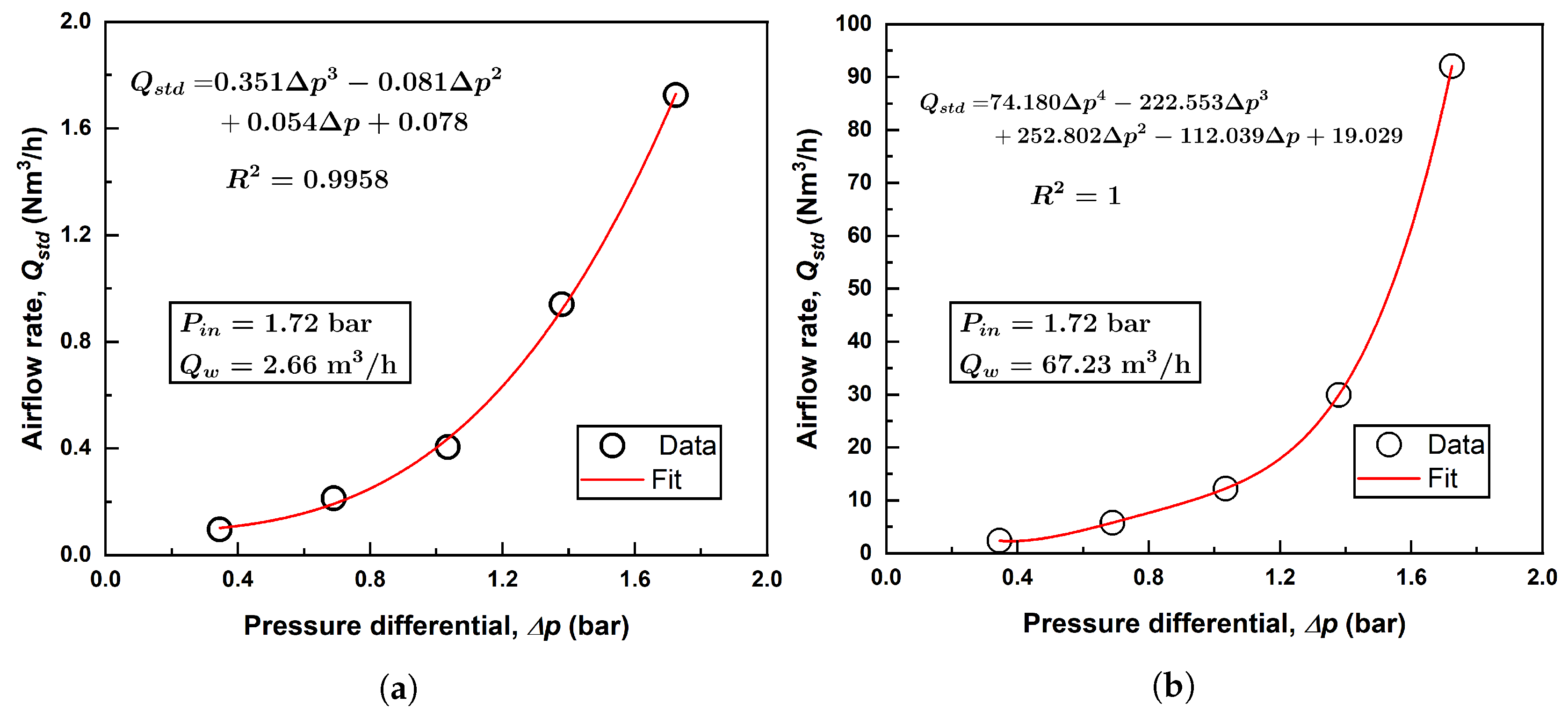
The outlet pressure of the Venturi injector is influenced by factors such as the pipe length and the properties of the two-phase mixture flowing through it. To accurately characterize this relationship, a suction flow rate versus pressure differential equation was developed from manufacturer data. To establish this relationship, manufacturer data were fitted with a 3rd-order polynomial. Figure 2 shows this relationship for an inlet pressure of 1.72 bar and two water flow rates (2.66 m3/h and 67.23 m3/h for the two injectors) to demonstrate how air flow rates are calculated.
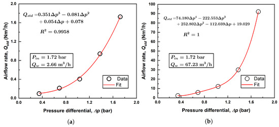
Figure 2.
Example polynomial fitting of air flow rate for (a) Model 1078; (b) Model 4091.
As previously mentioned, once a computational volume finishes its journey through the pipe, it is assumed to be homogeneously mixed with the tank, and the dissolved oxygen concentration is updated. This process continues until a steady-state concentration is reached. Figure 3 shows all major steps involved in the simulation.
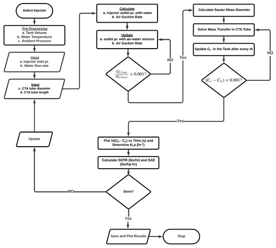
Figure 3.
Flowchart of the simulation procedure.
In the current work, only the hydraulic power developed by the pump is considered for the performance analysis of the system. The fluidic power delivered () by the pump, in kW, is estimated by the following equation, knowing the differential pressure and flow rate through the pump and noting that the pump pressure is expressed in bar:
In this analysis, water flow rate and pressure at the inlet of the injector at Point 4 in Figure 1 are utilized directly from manufacturer’s data. Since the pipe length and diameter are known, the energy equation between Points 3 and 4 in Figure 1 can be solved as in Equation (48):
Similarly, the pump’s inlet pressure can be calculated between Points 1 and 2 in Figure 1 as follows:
In these equations, elevation is measured from the bottom of the basin or tank. Since the tank is not pressurized and water in the tank is static, becomes 0 bar and is 0 m/s. The velocity from Points 3 to 4 is equivalent, and is the pressure at the injector inlet. includes frictional loss and minor losses from pipe fittings; its general expression is:
Thus, the pressure differential across the pump becomes:
2.5. Model Validation
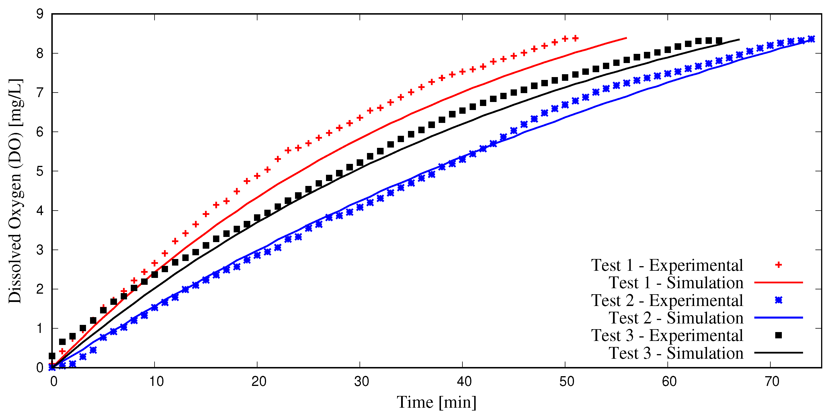
The simulation procedure outlined in this study was validated with three experiments. Here, a large container was filled with 946 liters of tap water at 25 °C and deoxygenated using anhydrous sodium sulfite (NA2SO3). Cobalt chloride (CoCl2) was used as a catalyst to speed up the reactions, and a starting DO content of 0 mg/L was achieved. Next, aeration was initiated using the Model 1078 (2.54 cm) injector, with motive flow provided by a 0.5 hp centrifugal pump. Pressure gauges and flow meters were employed to determine (water and air) flow rates and pressures necessary to conduct DBM simulations; see Figure 1. A 2.54 cm diameter coiled tube with a length of 6.1 m was employed as the confined tube aerator. Two Vernier DO probes (ODO-BTA) measured dissolved oxygen content as water was re-oxygenated. These values were averaged and recorded at one-minute intervals and compared to simulation results using the methodology presented herein, as seen in Figure 4.
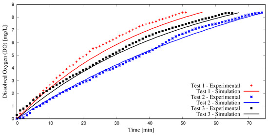
Figure 4.
Experimental validation of simulation methodology.
Three experimental tests were conducted using valve control to achieve different operational conditions, listed in Table 1.

Table 1.
Experimental conditions for validation of simulation methodology.
The results indicate that the methodology utilized in this study is adequate in predicting dissolved oxygen content and in most cases predicts DO values with less than 15% discrepancy between experiments and simulations. More details on the experimental procedure outlined herein may be found in [20].
3. Results and Discussion
Simulations were conducted using the aforementioned procedures for various water flow rates, inlet injector pressures, and CTA pipe lengths for both Model 1078 (2.54 cm) and Model 4091 (10.16 cm) injectors. As mentioned previously, air flow rates depend completely on water flow rates and pressure differential across the injector and are available from manufacturer’s data; an example of which is shown in Figure 2.
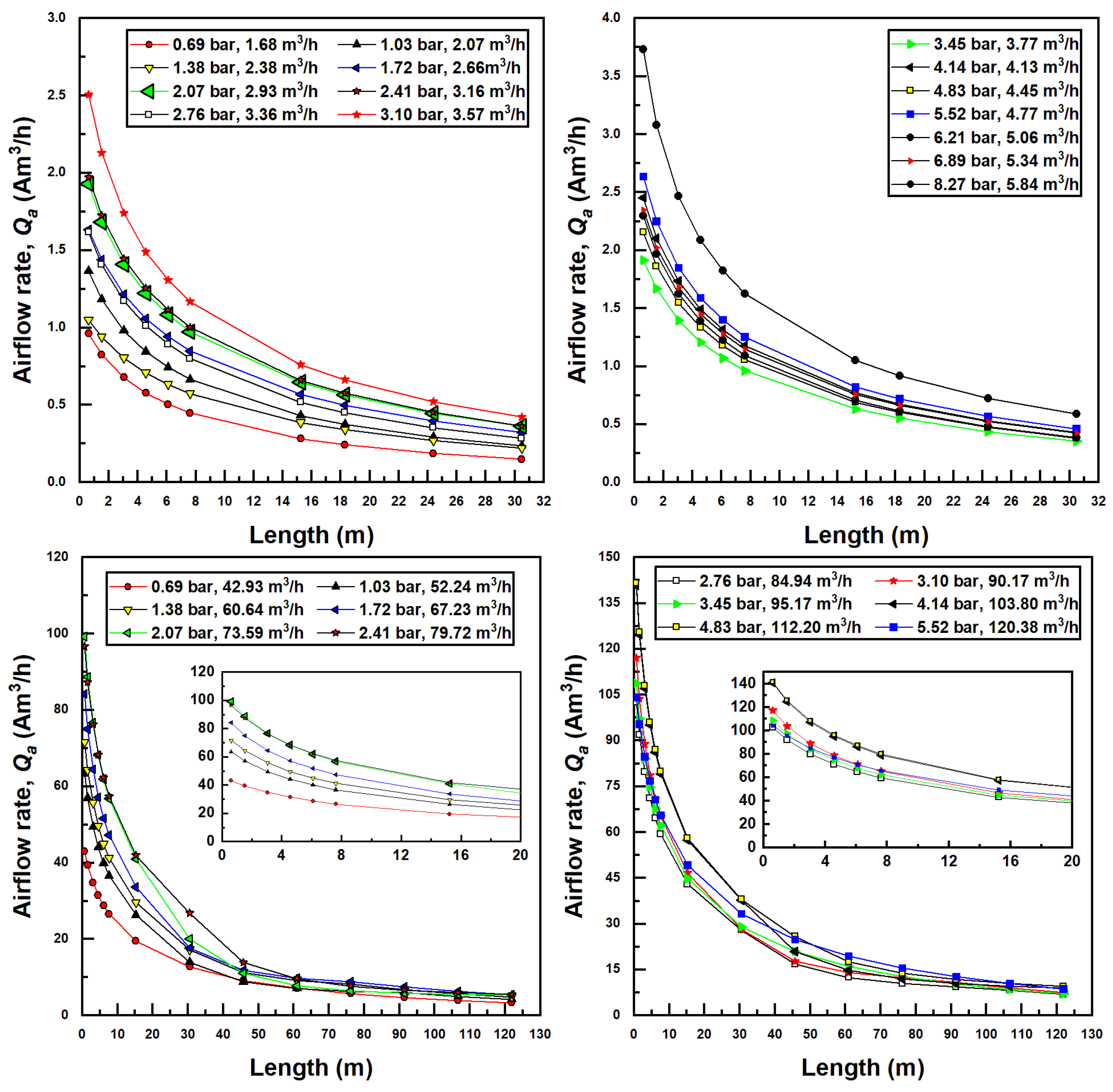
The pipe length, through the associated pressure drop due to viscous effects, affects the outlet pressure of the injector and thereby the pressure differential. Given a Venturi inlet pressure, a longer pipe forces a smaller pressure differential through the injector, which, in turn, decreases the air suction rate, which further affects the two-phase pressure drop through the pipe. Each simulation required an iterative procedure (seen in Figure 3) to converge to an appropriate pressure differential and air flow rate, given an inlet pressure and pipe length. As a result, for every simulation conducted, an increase in pipe length decreased the pressure differential across the injector. This, in turn, decreases the suction air flow rate, as seen in Figure 5.
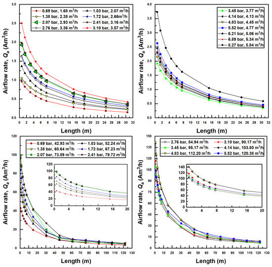
Figure 5.
Suction air flow (actual) rate dependence on confined tube length for various inlet pressures and water flow rates; Models 1078 (top two figures) and 4091 (bottom two figures).
Furthermore, apparent in Figure 5 is the fact that as inlet injector pressure increases, suction flow rates increase. This is due to the fact that a greater amount of pressure differential becomes available for the injector. Air flow rates increase with increased water flow rates as well due to the increased fluidic energy available to pull air into the injector. The larger (Model 4091) injector draws much more air than the smaller injector mainly for this reason.
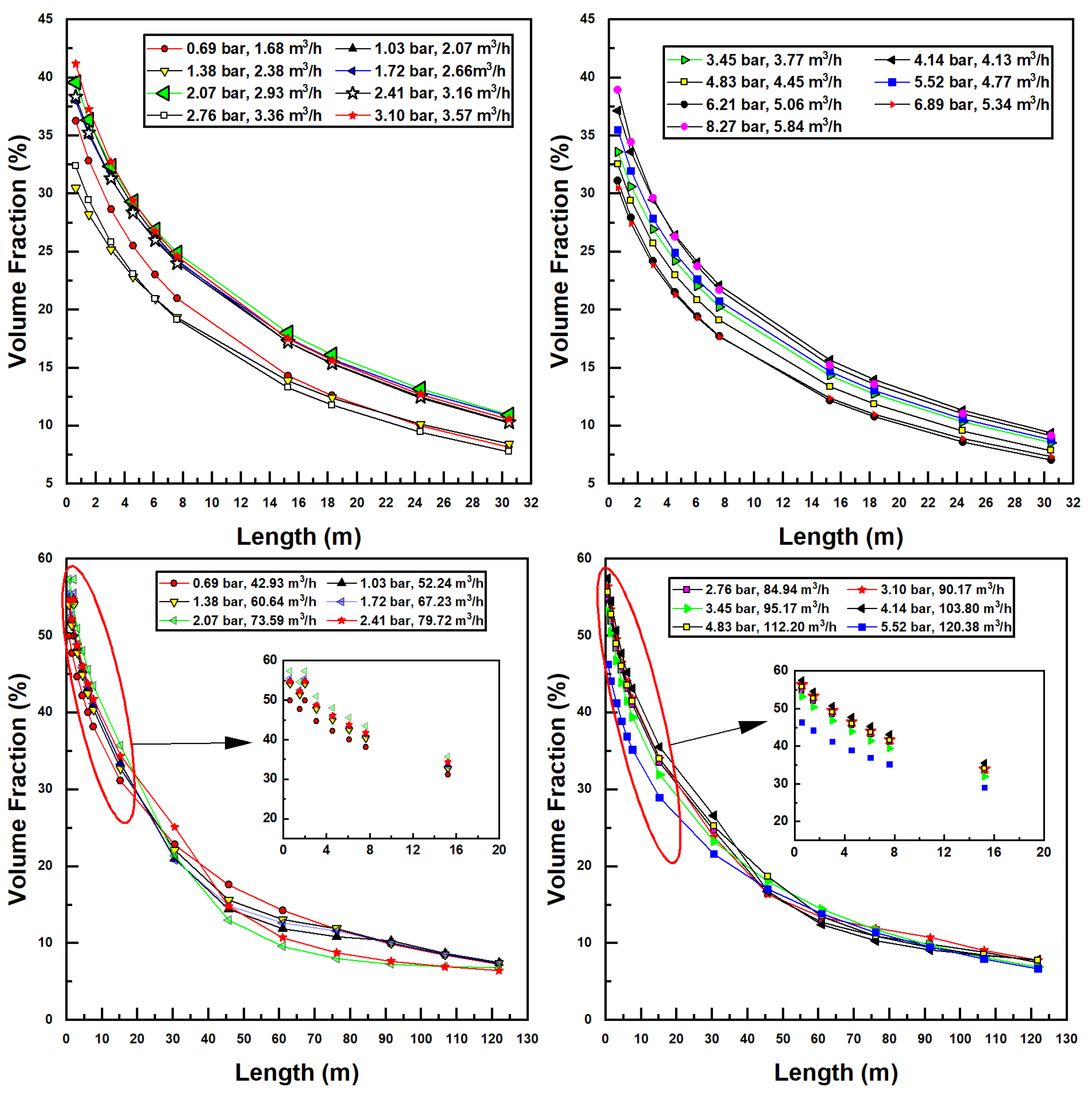
Since transfer is directly proportional to interfacial surface area, which is related to air and water flow rates within the pipe, the two injectors may be further compared according to the volume fraction of air within the pipe, which is calculated using Equation (12). All air volume fractions for simulations in this study are seen in Figure 6.
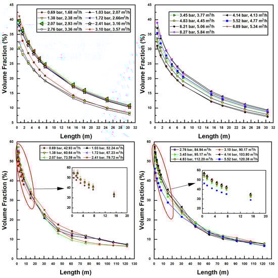
Figure 6.
Air volume fraction dependence on confined tube length for various inlet pressures and water flow rates; Models 1078 (top two figures) and 4091 (bottom two figures).
In Figure 6, similar trends are seen as with the previous discussion of air flow rates. Decreasing air volume fractions can be correlated with increased pipe lengths due to lower air flow. Interestingly, no discernible trend relating the air volume fraction to inlet pressure and flow rate can be discerned. This is perhaps due to the dimensionless nature of the volume fraction—a suitably nondimensionalized set of variables may prove these curves to collapse onto a single relationship. Equally interesting is the comparison between the two injector sizes. The larger model achieves higher air volume fractions than the smaller injector; a maximum of around 60% for Model 4091 versus 41% for Model 1078. This is likely due to the increase in available hydraulic power (larger flow rates are possible) combined with reduced frictional losses (as these scale with the square of velocity, which, for a given flow rate, decreases in an inverse-squared relationship with increased radius).
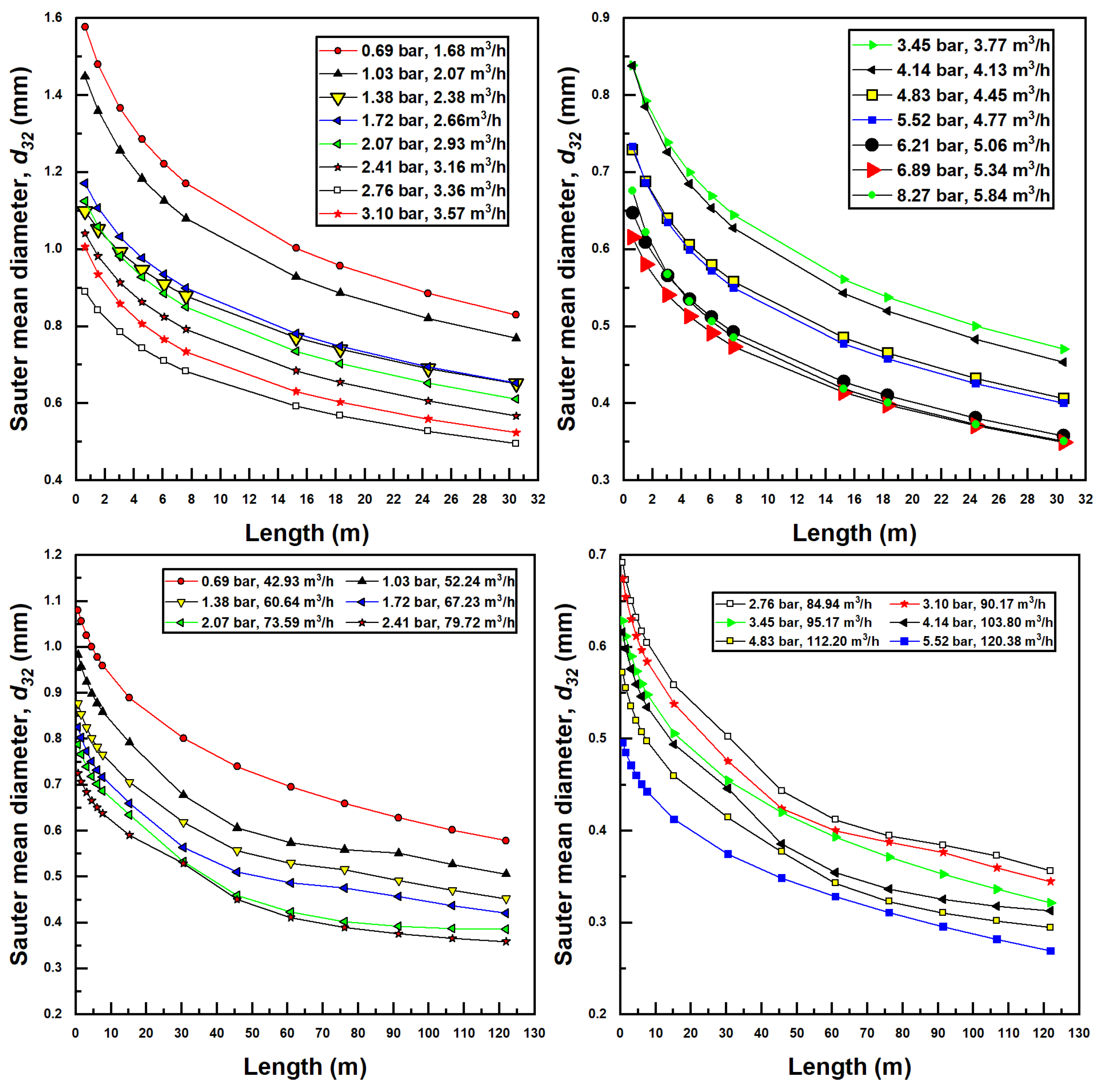
Of equal importance to the volumetric air flow rates and volume fractions is the bubble sizes; smaller bubble enable a larger surface area per unit air flow rate for mass transfer to occur. Recall that bubble sizes are calculated based on established nondimensional relationships [35] (see Equation (36)) and depend on water and air flow Reynolds numbers as well as the air-to-water ratio, which depends on the volumetric fraction as follows: .
Figure 7 shows the variation in Sauter mean diameter (SMD) for various confined tube length and for differing inlet pressures and flow rates for the two injectors investigated herein. It is observed here that an increase in liquid flow rate generally produces smaller bubbles. This is due to a more substantial pressure recovery (according to Bernoulli’s theorem) occurring in the diverging section of the injector, which is known to disassociate bubbles in Venturi injectors. With larger pressure recovery, bubbles generally shrink, and with less severe pressure recovery, bubbles generally grow in size. For this reason, the larger injector generally produces smaller bubbles.
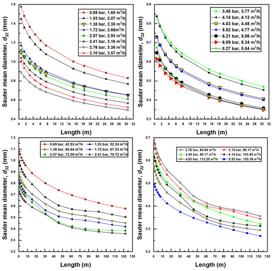
Figure 7.
Sauter mean diameter bubble production for various confined tube lengths and water inlet pressure and flow rates; Models 1078 (top two figures) and 4091 (bottom two figures).
Another interesting aspect of Figure 7 is that bubble sizes decrease with the increase in confined tube length. If inlet pressure and flow rate are held constant, it has already been established that an increase in CTA pipe length decreases air suction rates and gas volume fraction. This, in turn, decreases the air Reynolds number () as well as the gas fraction (). Drawing on Equation (36), these changes have the effect of decreasing the SMD (from a reduced ) while simultaneously increasing the SMD (from a reduced ). Ultimately, the dependence of SMD on the air Reynolds number is stronger, as noted by the greater magnitude of the exponent in Equation (36), resulting in an overall decreased SMD from the increased CTA pipe length.
Minimum SMD, experienced for each set of parameters at the longest CTA pipe lengths and at greatest flow rate and inlet pressure, were calculated to be around 0.35 mm for the smaller injector (Model 1078) and around 0.30 mm for the larger injector (Model 4091). Maximum SMD bubbles were experienced at the shortest CTA pipe lengths, and lowest inlet pressures and flow rates were calculated to be around 1.6 mm for the small injector and 1.1 mm for the large injector.
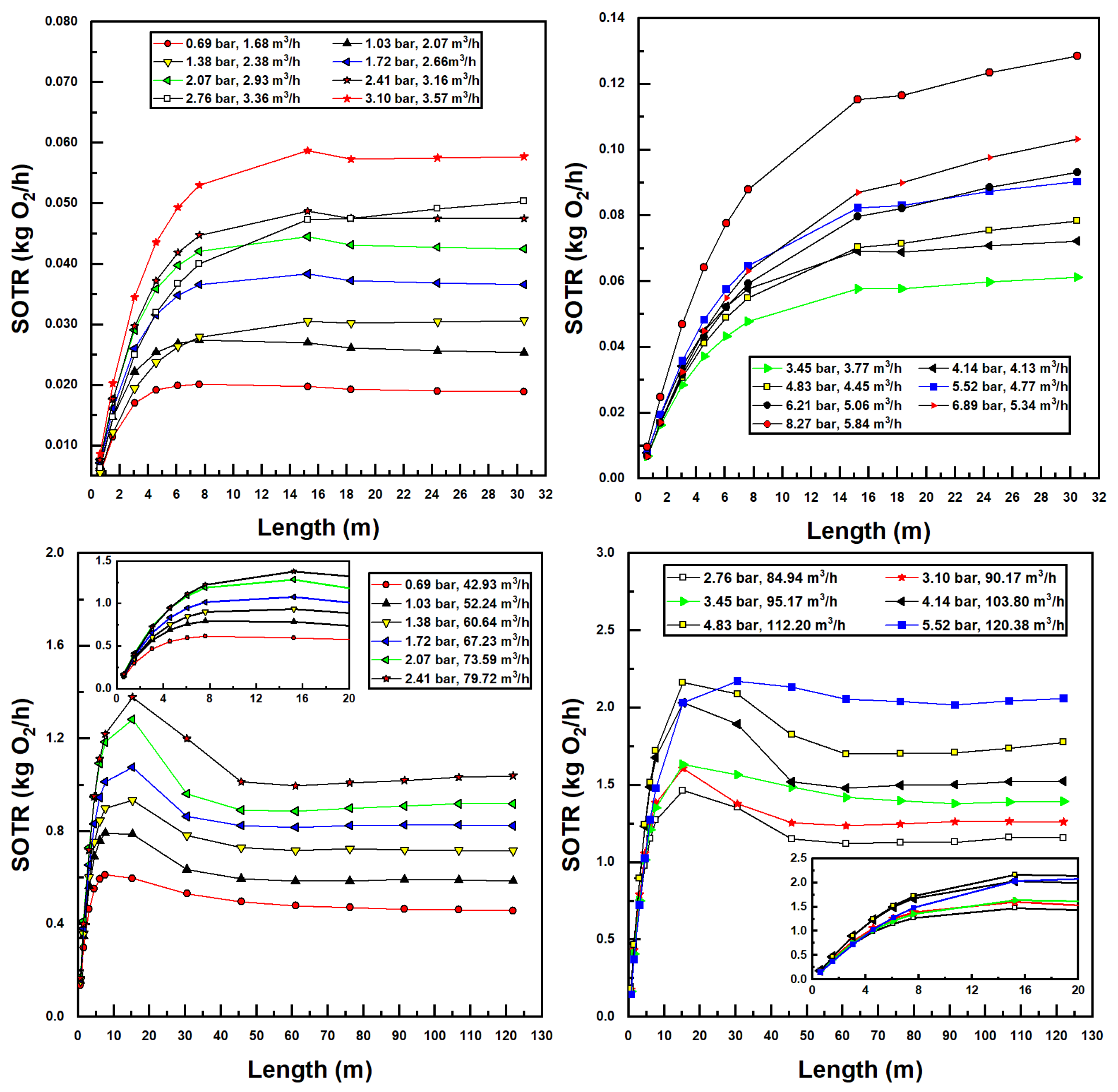
The bubble size, suction air fraction, injector inlet pressure, and flow rate, as well as CTA pipe length, all factor into the performance parameters of the aeration system, namely, the standard oxygen transfer rate (SOTR) and standard oxygen transfer efficiency (SAE). These parameters were calculated using Equations (17) and (18), the latter using developed power in the denominator calculated as the product of flow rate and pressure differential of water across the injector. Figure 8 displays all simulated SOTR values in this investigation.
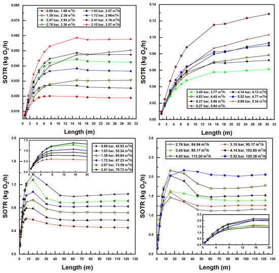
Figure 8.
Simulated standard oxygen transfer rate (SOTR) values for various confined tube lengths and water inlet pressure and flow rates; Models 1078 (top two figures) and 4091 (bottom two figures).
Some interesting observations can be made from the results in Figure 8. First and foremost, increasing water flow rates and inlet pressures increases SOTR. This is unsurprising, since increasing these two parameters increases the suction air flow rates (Figure 5) and decreases the bubble size (Figure 7), both trends acting to increase interfacial surface area and therefore mass transfer.
Additionally, it is evident in Figure 8 that, for small pipe lengths, increasing the pipe length increases SOTR. This is due to the fact that, at these small pipe lengths, there is insufficient residence time for entrained bubbles to transfer mass to the water; all plots achieve a SOTR of zero with zero pipe length since mass transfer in the tank is ignored. The rise in SOTR is quite evident at these smaller pipe lengths, due to the high concentration difference between air and water, which increases mass transfer rates. As pipe length increases, concentration differences decrease, while suction air flow rates and air fractions decrease simultaneously, until a maximum SOTR is encountered (in some instances), after which SOTR tends toward a relatively stable value. This trend can be expected, since sufficient increases in pipe length—while increasing bubble residence time—decrease the air suction fraction and therefore the SOTR. Interestingly, for the larger (Model 4091) injector, a clear maximum SOTR is reached for each pipe length with a given injector inlet pressure and flow rate—between 5 m and 30 m length in call cases. Bubble sizes are significantly lower—and air fractions higher—for this injector, as compared to the smaller (Model 1078) injector, making mass transfer considerably greater. Additionally, as the larger pipe size incurs lower frictional pressure drops, larger pipe lengths may be utilized within the operational envelope of these injectors, further increasing SOTR for the larger model. Lastly, the gradual flattening of SOTR data with the increased pipe length in Figure 8 is a result of approaching saturation concentration. In many instances—and especially for the larger injector model—bubble residence times are sufficient so that water becomes saturated with oxygen, preventing any further increases in SOTR.
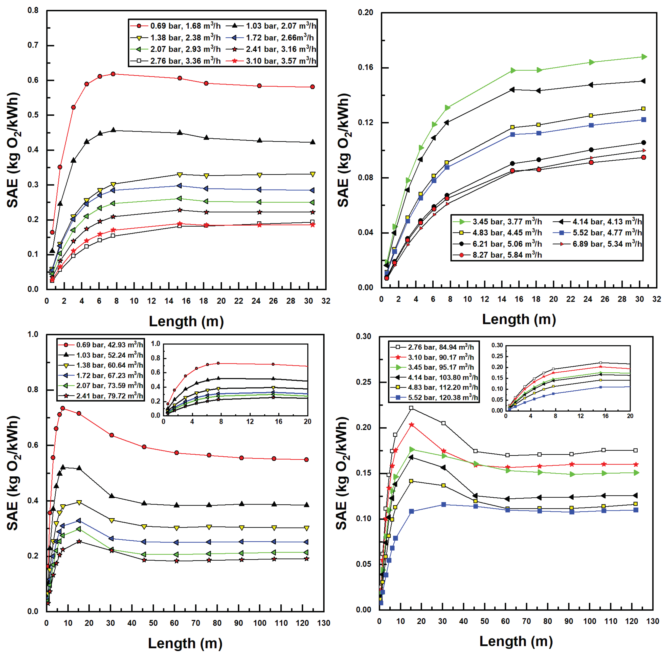
Standard Aeration Efficiency (SAE) trends are seen in Figure 9. SAE trends generally follow those of SOTR (Figure 8); however, those inlet injectors and pressures with the highest SOTR values achieve the lowest SAE values. This is due to the fact that SAE values are calculated by dividing SOTR by developed (fluidic) power, which is highest for high flow rates and pump differentials. As a result, from an energy efficiency perspective, lower flow rates and injector input pressures are more desirable. Maximum SAE values reported were 0.74 kgO2/kWh for Model 4091 and 0.62 kgO2/kWh for Model 1078. These values are generally in the range of those found in recent studies [16,17,18,19] with maximal SAE reported herein being slightly higher due to the use of the novel CTA assembly to assist aeration.
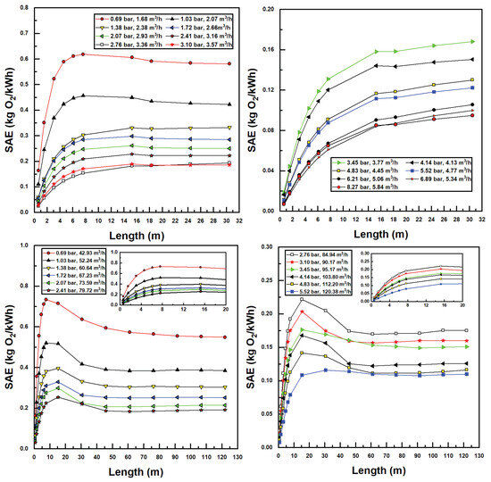
Figure 9.
Simulated standard aeration efficiency (SAE) values for various confined tube lengths and water inlet pressure and flow rates; Models 1078 (top two figures) and 4091 (bottom two figures).
These results indicate that the CTA system scales well with increased diameter and power requirements in terms of system efficiency. Additionally, having knowledge of injector performance metrics allows this methodology to estimate the maximum aeration efficiency of the system with respect to confined tube pipe length, inlet injector pressure, and motive (water) flow rates, without the need for time-consuming and costly aeration experiments.
4. Conclusions
A novel microbubble aeration system is proposed herein, incorporating a Venturi injector and a coiled tube intended to facilitate bubble residence time without bubble coalescence. The proposed aeration system has the benefit of producing the interfacial area required for effective mass transfer without the need for compressors or blowers and deep aeration basins. Using manufacturer’s data for two injectors (2.54 cm and 10.16 cm diameter), along with nondimensional correlations available from recent studies to predict bubble sizes, air suction rates, air volumetric fractions, standard oxygen transfer rate (SOTR), and standard aeration efficiency (SAE) calculations were performed based on simulations using the discrete bubble model concept. The general results of this study are as follows:
- The proposed aeration system is capable of producing bubbles in the range of 0.15–1.58 mm for Model 1078 and 0.14–1.1 mm for Model 4091.
- Increases in water flow rates effectively increase the volume fraction of injected air. Maximum volume fraction varied between 40 and 60% for the injectors investigated, with the larger-diameter model enjoying larger maximal air volume fractions.
- Increasing the liquid flow rate improves the oxygen transfer rate through the system, due to decreases in bubble sizes and increases in injected air volume fraction.
- Increasing the liquid flow rate increases the power requirements. As a result, the system operates with lower energy consumption and higher standard aeration efficiency at lower water and pressure at the injector inlet.
- The confined tube length has a significant impact on the oxygen transfer rate—longer pipe lengths can effectively improve bubble residence times, increasing mass transfer. However, too long of a pipe decreases the suction air flow rates and increases viscous losses significantly, affecting standard aeration efficiency negatively. For each injector investigated, a maximal standard aeration efficiency was found with respect to pipe length. This was found to be 0.74 kgO2/kWh for the larger (10.16 cm) injector and CTA assembly, compared to 0.62 kgO2/kWh. Both of these values were higher than those found in the recent literature concerning traditional Venturi aeration.
Further studies are underway to investigate the relative cost of bubble production in Venturi injectors on the basis of energy (pressure) losses for CTA applications, as they relate to the competing effects of viscous losses in the coiled pipes themselves, at larger diameters in varying configurations. Other future works in this area, some of which are intended to address limitations of this study, are as follows:
- Addressing bubble agglomeration/breakup, which may become especially important as aeration tubes become larger and potentially slower-moving.
- Analysis of effects of radius of curvature, which may affect frictional pressure drop at low radii.
- Parallelization of Venturi injectors and aeration tubes, which may prove beneficial at larger scales necessary for municipal wastewater treatment.
- Analysis of system performance when clean water is replaced with a mixed-liquor fluid typically seen in wastewater aeration basins.
The results of this study are encouraging, especially given that increases in aeration efficiency were found for an increased injector diameter and, hence, the system capacity for delivering oxygen to wastewater. Since traditional Venturi aeration in wastewater applications is currently focused on ejecting the air/water mixture in the bottoms of large basins, relying on smaller bubbles’ increased residence time to increase oxygen transfer, this study represents a fundamental shift in the application of Venturi injectors for wastewater treatment applications.
Author Contributions
Methodology and writing, R.M.; review and editing, J.C.; supervision and editing, D.W.M. All authors have read and agreed to the published version of the manuscript.
Funding
This research was partially funded by the United States Department of Energy’s Industrial Assessment Centers, grant number DE-FOA-0002452.
Data Availability Statement
Data are contained within the article.
Conflicts of Interest
The authors declare no conflict of interest.
References
- Henderson, M. Energy Reduction Methods in the Aeration Process at Perth Waste Water Treatment Plant. Renewable Energy Systems and the Environment. Master’s Thesis, University of Strathclyde, Glasgow, UK, 2002. [Google Scholar]
- Rosso, D.; Stenstrom, M.K. Alpha factors in full-scale wastewater aeration systems. Proc. Water Environ. Fed. 2006, 7, 4853–4863. [Google Scholar] [CrossRef]
- Terasaka, K.; Hirabayashi, A.; Nishino, T.; Fujioka, S.; Kobayashi, D. Development of microbubble aerator for waste water treatment using aerobic activated sludge. Chem. Eng. Sci. 2011, 66, 3172–3179. [Google Scholar] [CrossRef]
- Nadayil, J.; Mohan, D.; Dileep, K.; Rose, M.; Parambi, R.R.P. A study on effect of aeration on domestic wastewater. Int. J. Interdiscip. Res. Innov. 2015, 3, 10–15. [Google Scholar]
- Ahmad, N.; Javed, F.; Awan, J.A.; Ali, S.; Fazal, T.; Hafeez, A.; Aslam, R.; Rashid, N.; Rehman, M.S.U.; Zimmerman, W.B.; et al. Biodiesel production intensification through microbubble mediated esterification. Fuel 2019, 253, 25–31. [Google Scholar] [CrossRef]
- Jenkins, T.E. Aeration Control System Design: A practical Guide to Energy and Process Optimization; John Wiley & Sons: Hoboken, NJ, USA, 2013. [Google Scholar]
- Shammas, N.K. Fine pore aeration of water and wastewater. In Advanced Physicochemical Treatment Technologies; Springer: Berlin/Heidelberg, Germany, 2007; pp. 391–448. [Google Scholar]
- Hafeez, A.; Shamair, Z.; Shezad, N.; Javed, F.; Fazal, T.; Ur Rehman, S.; Bazmi, A.A.; Rehman, F. Solar powered decentralized water systems: A cleaner solution of the industrial wastewater treatment and clean drinking water supply challenges. J. Clean. Prod. 2021, 289, 125717. [Google Scholar] [CrossRef]
- Rosso, D.; Larson, L.E.; Stenstrom, M.K. Aeration of large-scale municipal wastewater treatment plants: State of the art. Water Sci. Technol. 2008, 57, 973–978. [Google Scholar] [CrossRef]
- Basso, A.; Hamad, F.; Ganesan, P. Effects of the geometrical configuration of air–water mixer on the size and distribution of microbubbles in aeration systems. Asia-Pac. J. Chem. Eng. 2018, 13, e2259. [Google Scholar] [CrossRef]
- Gourich, B.; Azher, N.E.; Vial, C.; Soulami, M.B.; Ziyad, M.; Zoulalian, A. Influence of operating conditions and design parameters on hydrodynamics and mass transfer in an emulsion loop-venturi reactor. Chem. Eng. Process. Process Intensif. 2007, 46, 139–149. [Google Scholar] [CrossRef]
- Yoshida, A.; Takahashi, O.; Ishii, Y.; Sekimoto, Y.; Kurata, Y. Water purification using the adsorption characteristics of microbubbles. Jpn. J. Appl. Phys. 2008, 47, 6574. [Google Scholar] [CrossRef]
- Zhao, L.; Mo, Z.; Sun, L.; Xie, G.; Liu, H.; Du, M.; Tang, J. A visualized study of the motion of individual bubbles in a venturi-type bubble generator. Prog. Nucl. Energy 2017, 97, 74–89. [Google Scholar] [CrossRef]
- Kadzinga, F. Venturi Aeration of Bioreactors. Master’s Thesis, University of Cape Town, Cape Town, South Africa, 2015. [Google Scholar]
- West, H.S. Apparatus and Method for Introducing a Gas into a Liquid. U.S. Patent 13/379,441, 28 June 2012. [Google Scholar]
- Yadav, A.; Kumar, A.; Sarkar, S. Performance evaluation of venturi aeration system. Aquac. Eng. 2021, 93, 102156. [Google Scholar] [CrossRef]
- Dong, C.; Zhu, J.; Wu, X.; Miller, C.F. Aeration efficiency influenced by venturi aerator arrangement, liquid flow rate and depth of diffusing pipes. Environ. Technol. 2012, 33, 1289–1298. [Google Scholar] [CrossRef]
- Zhu, J.; Miller, C.F.; Dong, C.; Wu, X.; Wang, L.; Mukhtar, S. Aerator module development using venturi air injectors to improve aeration efficiency. Appl. Eng. Agric. 2007, 23, 661–667. [Google Scholar] [CrossRef]
- Dange, A.; Warkhedkar, R. An experimental study of venturi aeration system. Mater. Today: Proc. 2023, 72, 615–621. [Google Scholar] [CrossRef]
- Mahmud, R.; Erguvan, M.; MacPhee, D.W. Performance of closed loop venturi aspirated aeration system: Experimental study and numerical analysis with discrete bubble model. Water 2020, 12, 1637. [Google Scholar] [CrossRef]
- MacPhee, D.W. Confined Tube Aspiration Aeration Devices and Systems. U.S. Patent 11,318,432, 3 May 2022. [Google Scholar]
- Baker, O. Design of pipelines for the simultaneous flow of oil and gas. In Proceedings of the SPE Annual Technical Conference and Exhibition, SPE, Dallas, TX, USA, 18–21 October 1953; p. SPE-323. [Google Scholar]
- Hetsroni, G. Handbook of Multiphase Systems; McGraw Hill: New York, NY, USA, 1982. [Google Scholar]
- Friedel, L. Improved friction pressure drop correlations for horizontal and vertical two-phase pipe flow. In Proceedings of the European Two-Phase Flow Group Meeting, Ispra, Italy, 5–8 June 1979. [Google Scholar]
- Colebrook, C.F. Turbulent flow in pipes, with particular reference to the transition region between the smooth and rough pipe laws. J. Inst. Civ. Eng. 1939, 11, 133–156. [Google Scholar] [CrossRef]
- Lewis, W.K.; Whitman, W.G. Principles of Gas Absorption. Ind. Eng. Chem. 2002, 16, 1215–1220. [Google Scholar] [CrossRef]
- ASCE. Standard Guidelines for In-Process Oxygen Transfer Testing; Technical Report; ASCE: Reston, VA, USA, 1997. [Google Scholar]
- ASCE. Measurement of Oxygen Transfer in Clean Water; American Society of Civil Engineers: Reston, VA, USA, 1993. [Google Scholar]
- McGinnis, D.F.; Little, J.C. Predicting diffused-bubble oxygen transfer rate using the discrete-bubble model. Water Res. 2002, 36, 4627–4635. [Google Scholar] [CrossRef]
- Cengel, Y.; Heat, T.M. Heat and Mass Transfer: A Practical Approach, 2nd ed.; McGraw Hill: New York, NY, USA, 2003. [Google Scholar]
- Griffith, R. Mass transfer from drops and bubbles. Chem. Eng. Sci. 1960, 12, 198–213. [Google Scholar] [CrossRef]
- Lochiel, A.; Calderbank, P. Mass transfer in the continuous phase around axisymmetric bodies of revolution. Chem. Eng. Sci. 1964, 19, 471–484. [Google Scholar] [CrossRef]
- Guggenheim, E.A. Thermodynamics: An Advanced Treatise for Chemists and Physicists; North-Holland Publishing Company: Amsterdam, The Netherlands, 1967. [Google Scholar]
- Sauter, J. Determining Size of Drops in Fuel Mixture of Internal Combustion Engines; No. NACA-TM-390; NACA: Washington, DC, USA, 1926. [Google Scholar]
- Gordiychuk, A.; Svanera, M.; Benini, S.; Poesio, P. Size distribution and Sauter mean diameter of micro bubbles for a Venturi type bubble generator. Exp. Therm. Fluid Sci. 2016, 70, 51–60. [Google Scholar] [CrossRef]
- Weiss, R. The solubility of nitrogen, oxygen and argon in water and seawater. In Deep Sea Research and Oceanographic Abstracts; Elsevier: Amsterdam, The Netherlands, 1970; Volume 17, pp. 721–735. [Google Scholar]
- Wüest, A.; Brooks, N.H.; Imboden, D.M. Bubble plume modeling for lake restoration. Water Resour. Res. 1992, 28, 3235–3250. [Google Scholar] [CrossRef]

Disclaimer/Publisher’s Note: The statements, opinions and data contained in all publications are solely those of the individual author(s) and contributor(s) and not of MDPI and/or the editor(s). MDPI and/or the editor(s) disclaim responsibility for any injury to people or property resulting from any ideas, methods, instructions or products referred to in the content. |
© 2024 by the authors. Licensee MDPI, Basel, Switzerland. This article is an open access article distributed under the terms and conditions of the Creative Commons Attribution (CC BY) license (https://creativecommons.org/licenses/by/4.0/).