

Simultaneous Optimization of Work and Heat Exchange Networks


Abstract
:1. Introduction
2. Problem Formulation
- Steady-state operation is considered.
- All process streams are ideal gaseous streams.
- Compression and expansion are reversible and adiabatic (i.e., isentropic).
- Expansion through the valve is isenthalpic with a constant Joule–Thompson coefficient.
- One hot and one cold utility is assumed.
- The compressor and expander isentropic efficiency is considered constant.
- The heat capacity flow rates are constant.
- Heat and pressure losses are neglected.
- The costs of mixers and expansion valves are negligible.
3. Methodology
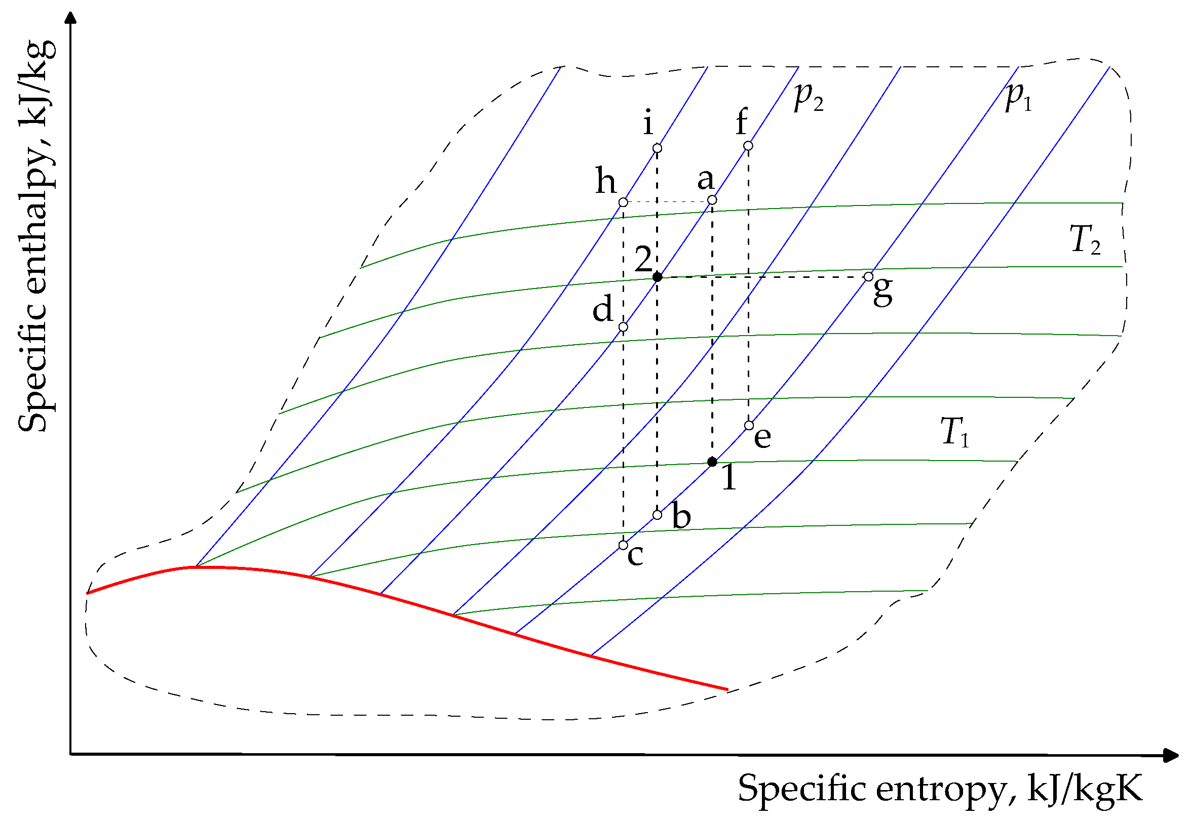
3.1. Possible Thermodynamic Paths
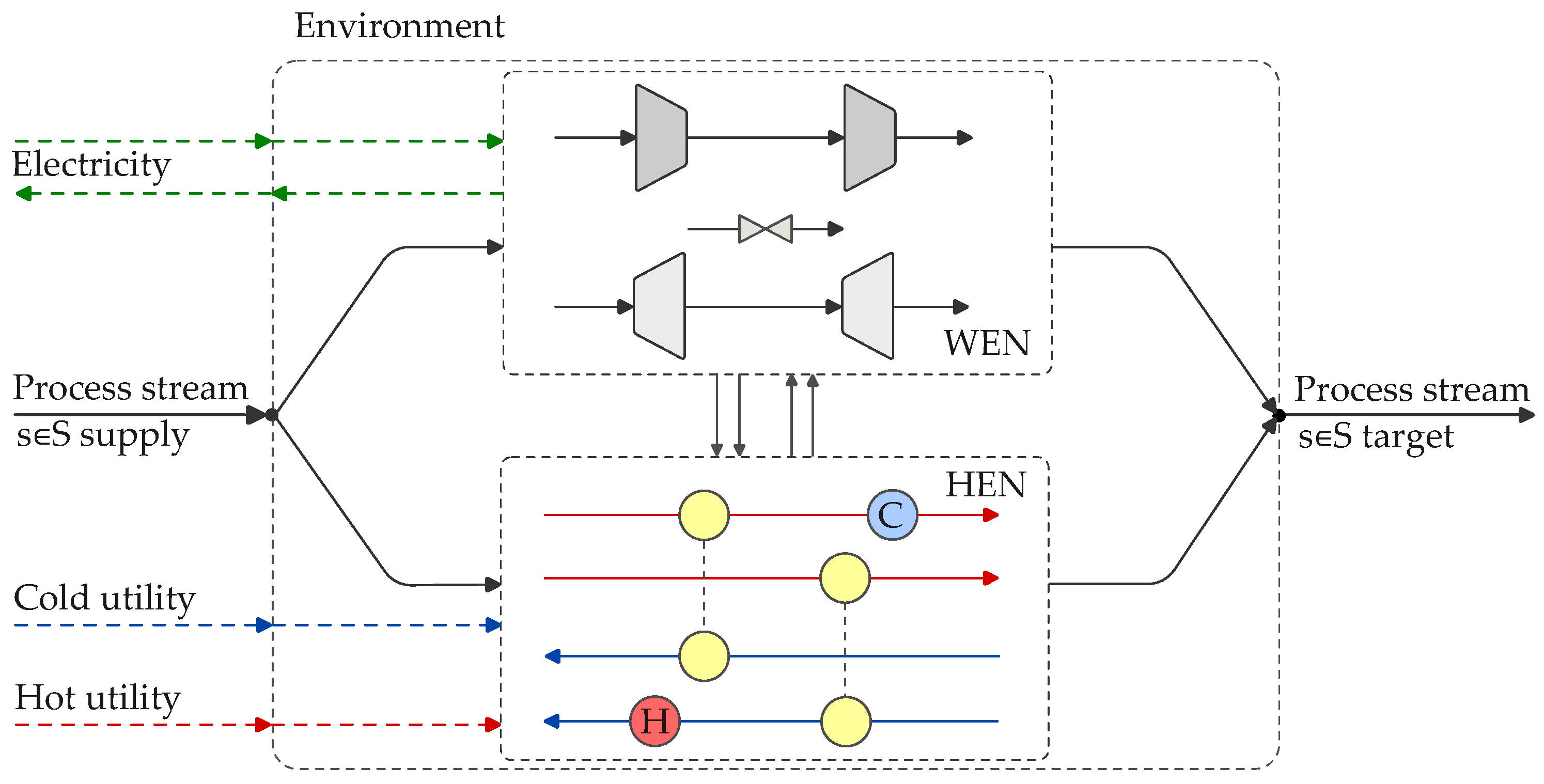
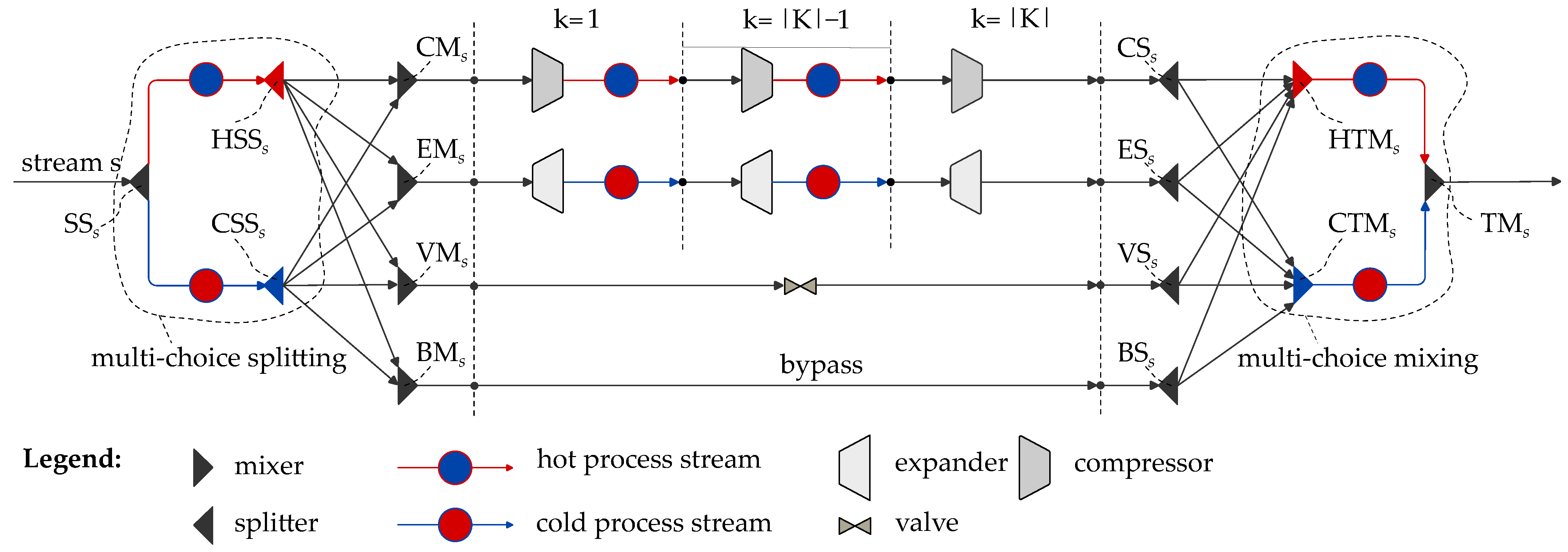
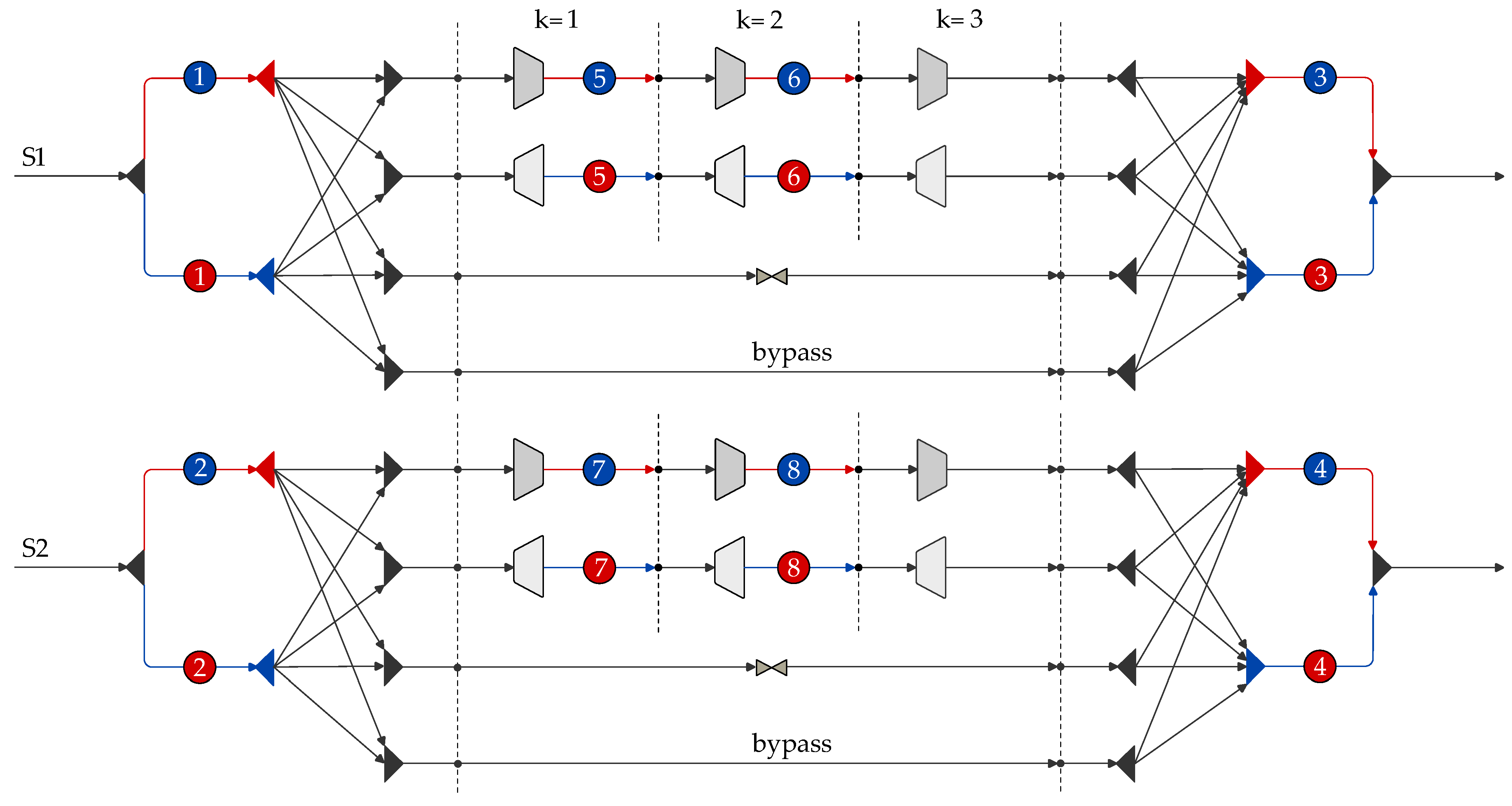
3.2. Work and Heat Integration (WHI) Superstructure
- SSs Supply splitter for stream s;
- HSSs Supply splitter for a potential hot stream s;
- CSSs Supply splitter for a potential cold stream s;
- CMs Mixer before compressor for stream s;
- EMs Mixer before expander for stream s;
- VMs Mixer before valve for stream s;
- BMs Mixer before bypass for stream s.
- HTMs Target mixer for a potential hot stream s;
- CTMs Target mixer for a potential cold stream s;
- TMs Target mixer for stream s.
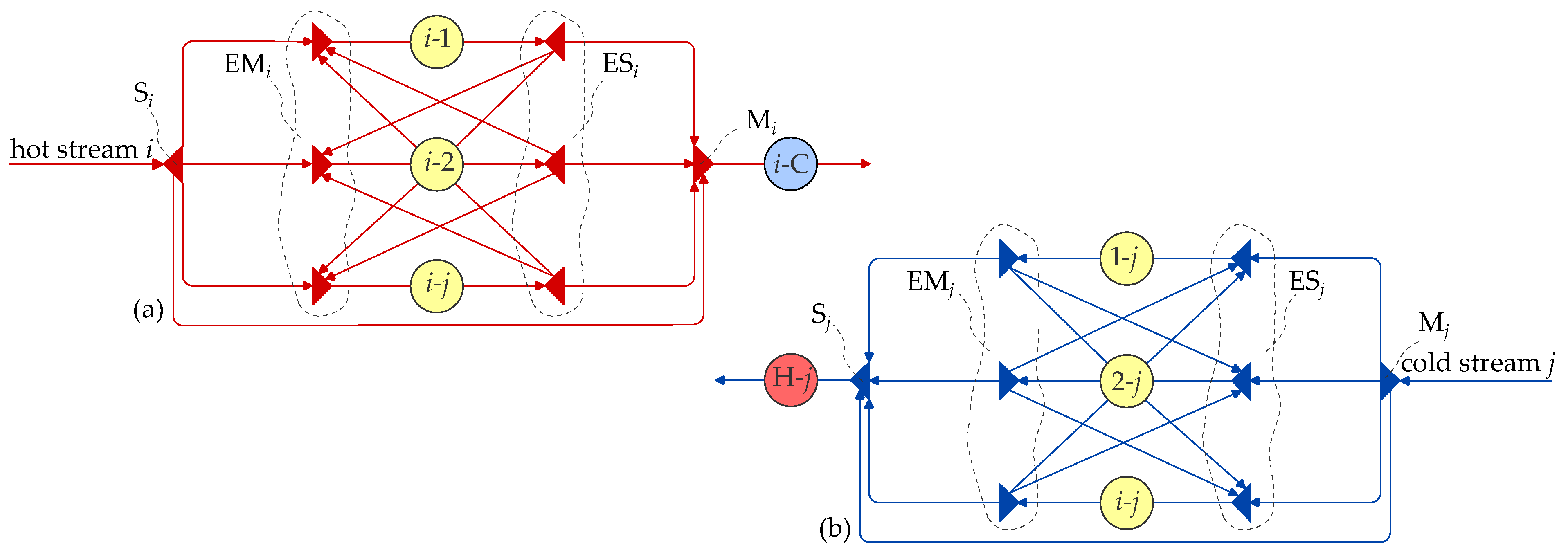
3.3. Heat Exchanger Network (HEN) Superstructure
3.4. Model
3.4.1. The Thermodynamic Path Model
3.4.2. The HI Model
3.4.3. The HEN Model
3.5. Objective Function
3.6. Model Limitations and Possible Improvements
- The model only includes pressure manipulation equipment for gaseous streams; to include liquid streams, additional pressure change branches should be included to enable the pumping of fluids and liquid expansion.
- Only one hot and one cold utility is considered, suggesting that the model’s extension should integrate the WHEN network with the utility network, enabling the extraction of utilities at different temperature levels.
- Only utility expanders and compressors are considered; there is a need to include SSTCs to enable additional work integration opportunities.
- Realistic efficiencies of compressors and expanders should be considered.
- The phase change (evaporation/condensation) should be considered.
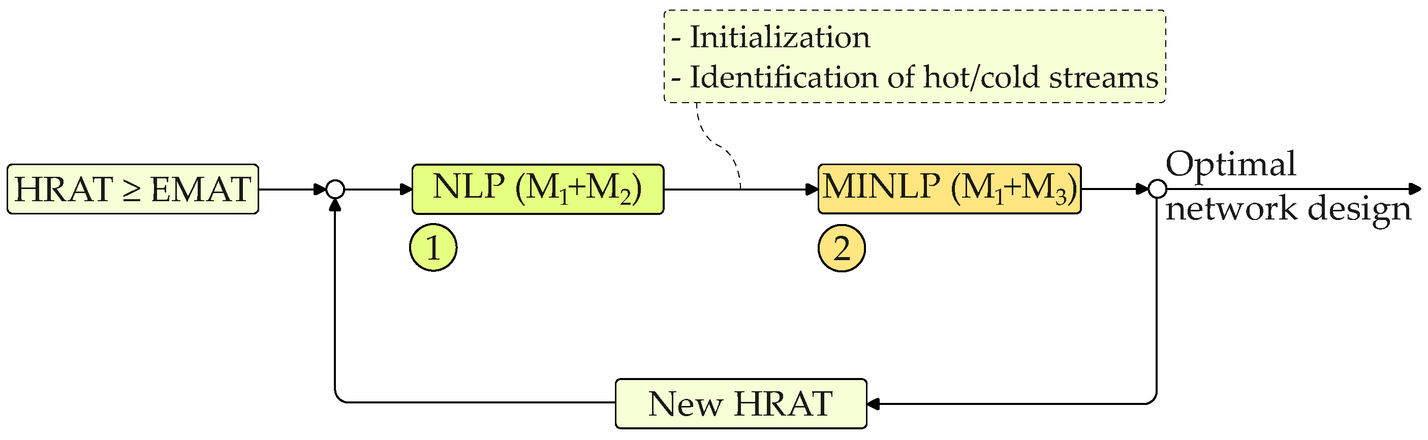
3.7. Solution Approach
4. Examples
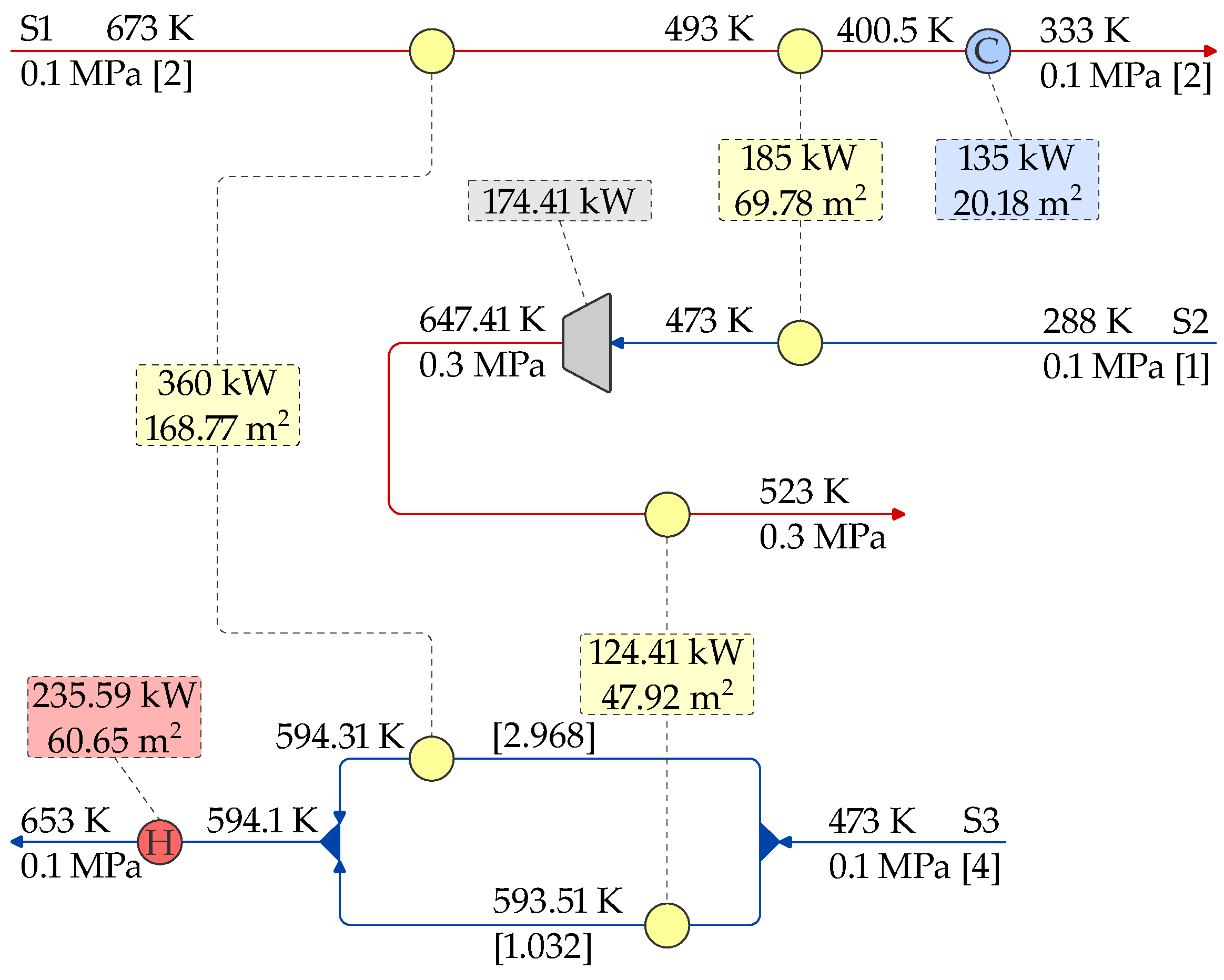
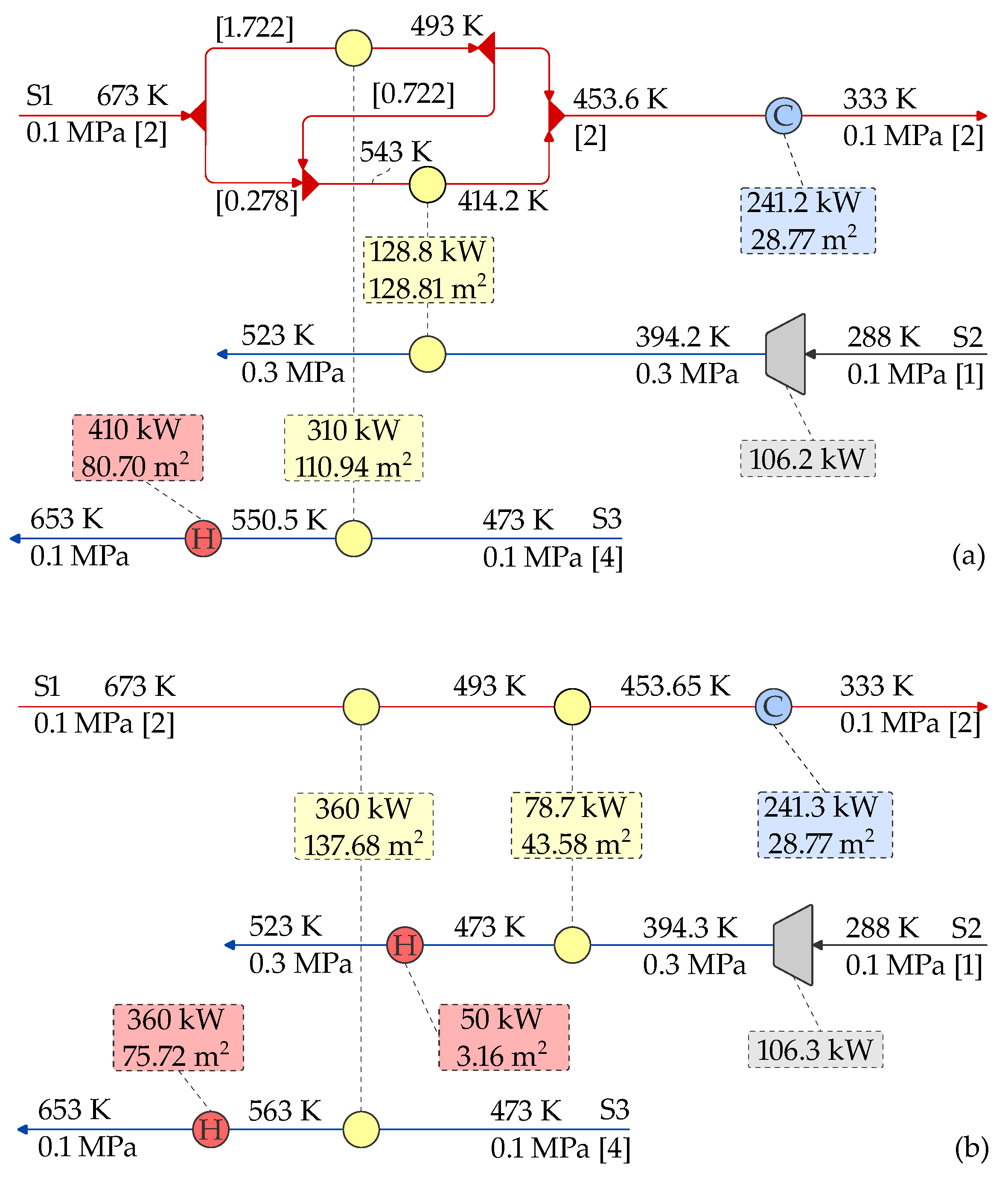
4.1. Example 1
4.2. Example 2
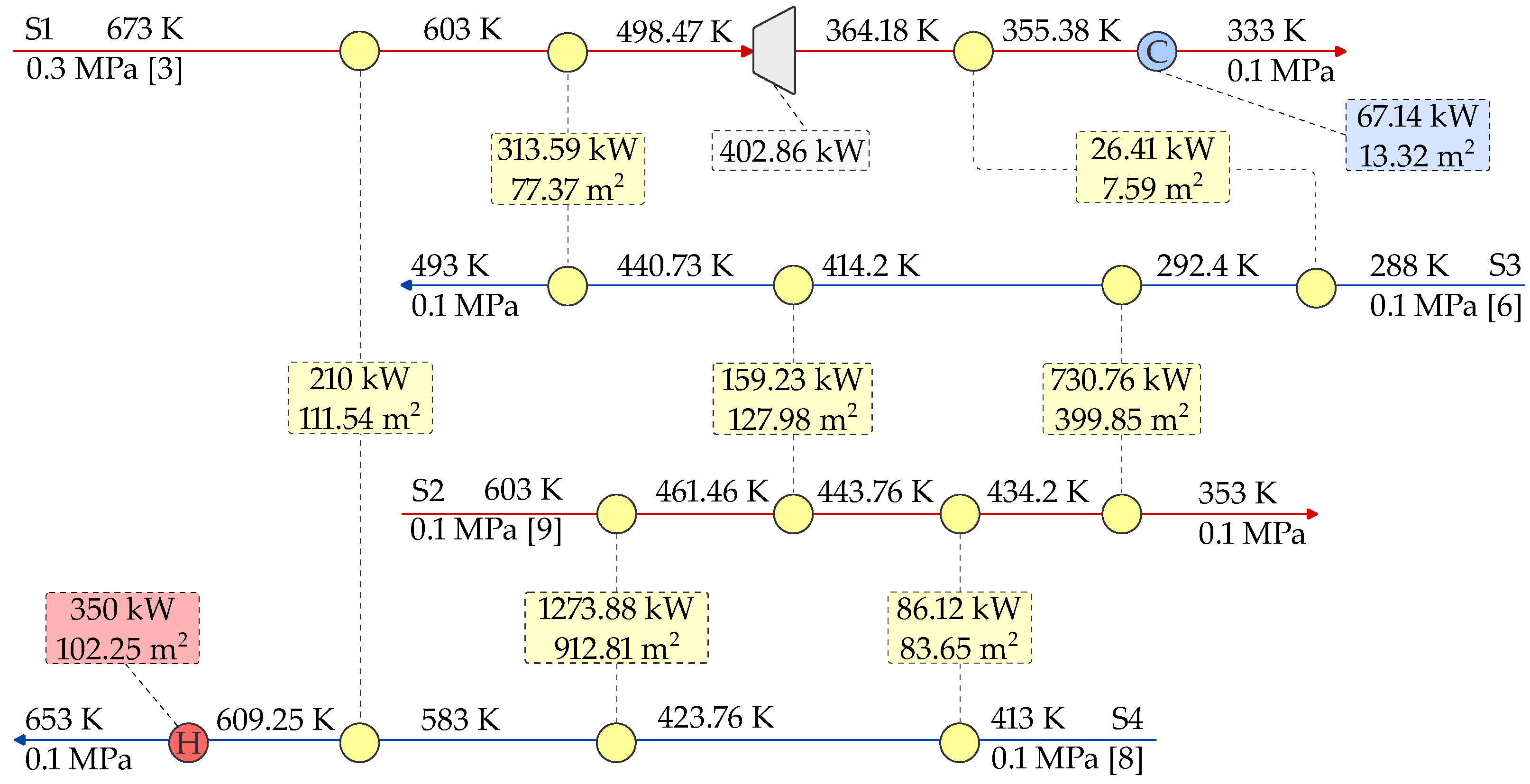
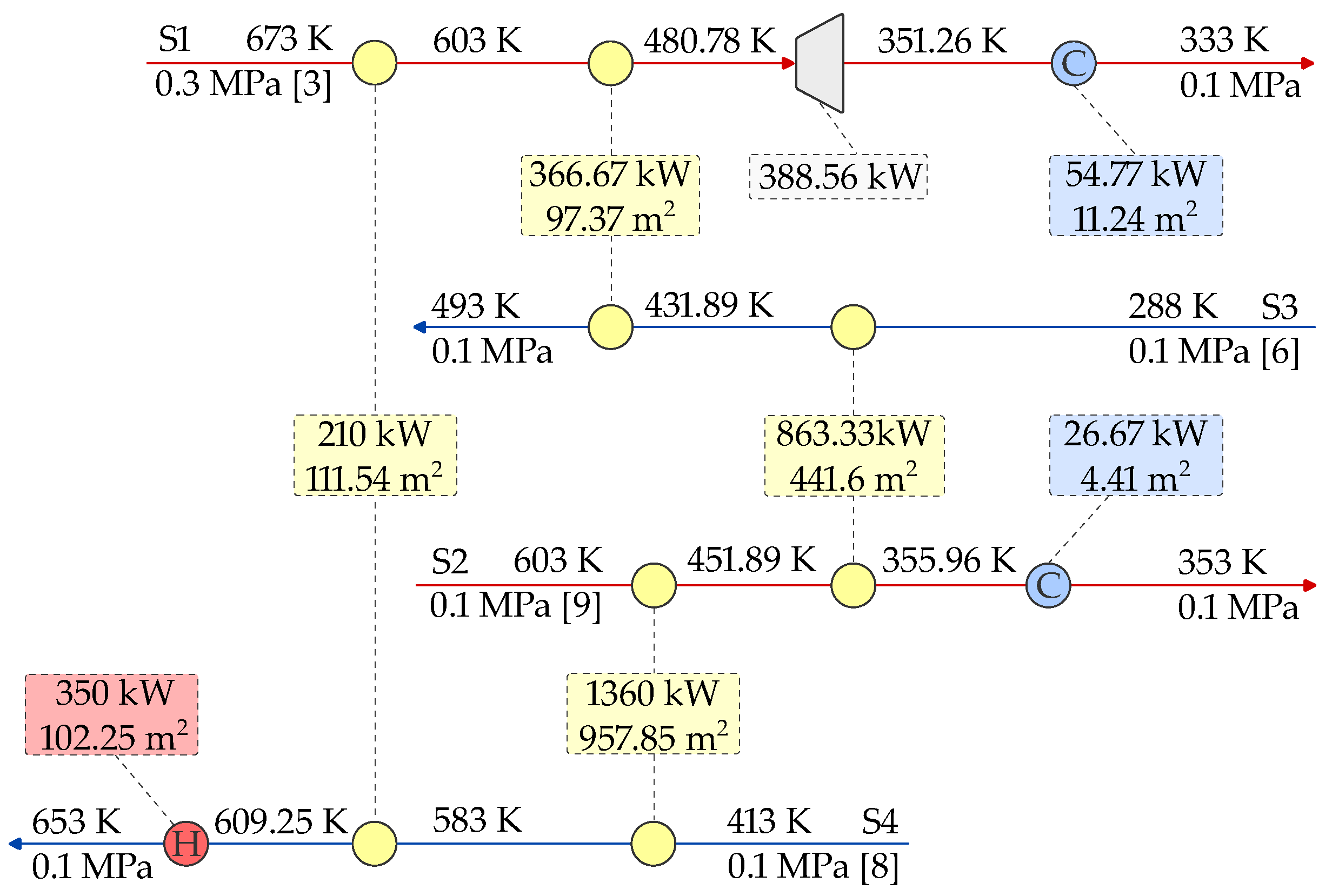
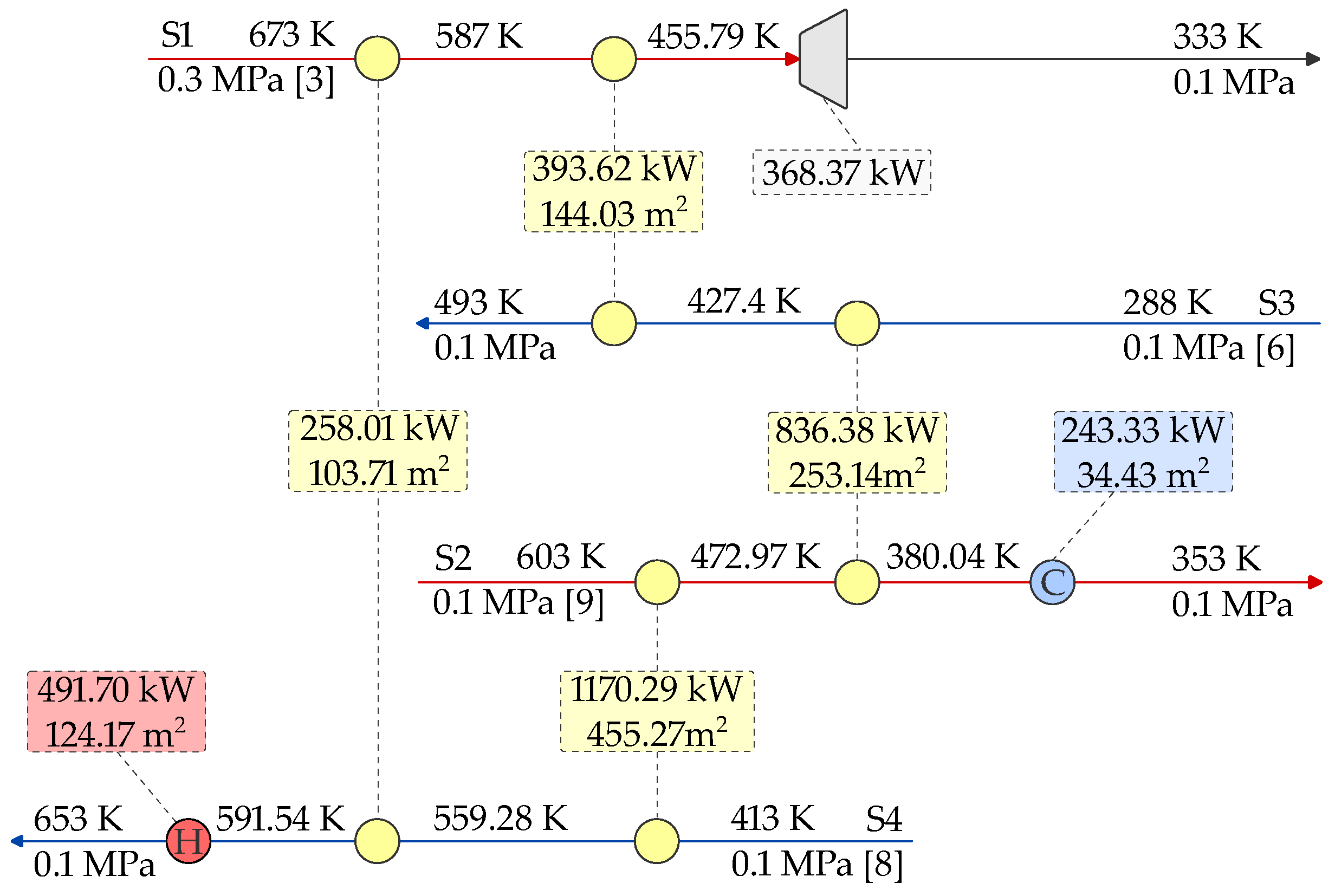
4.3. Example 3
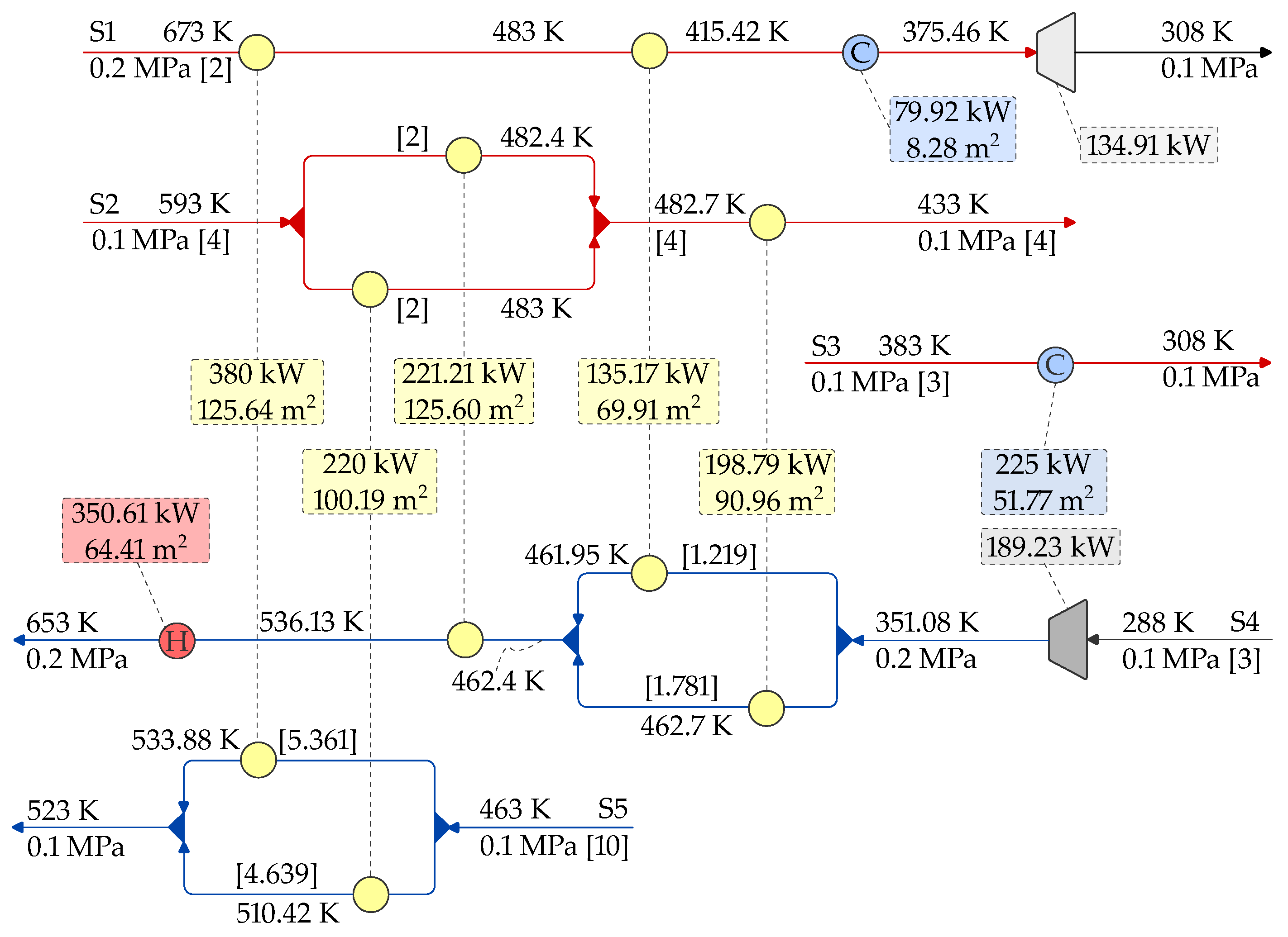
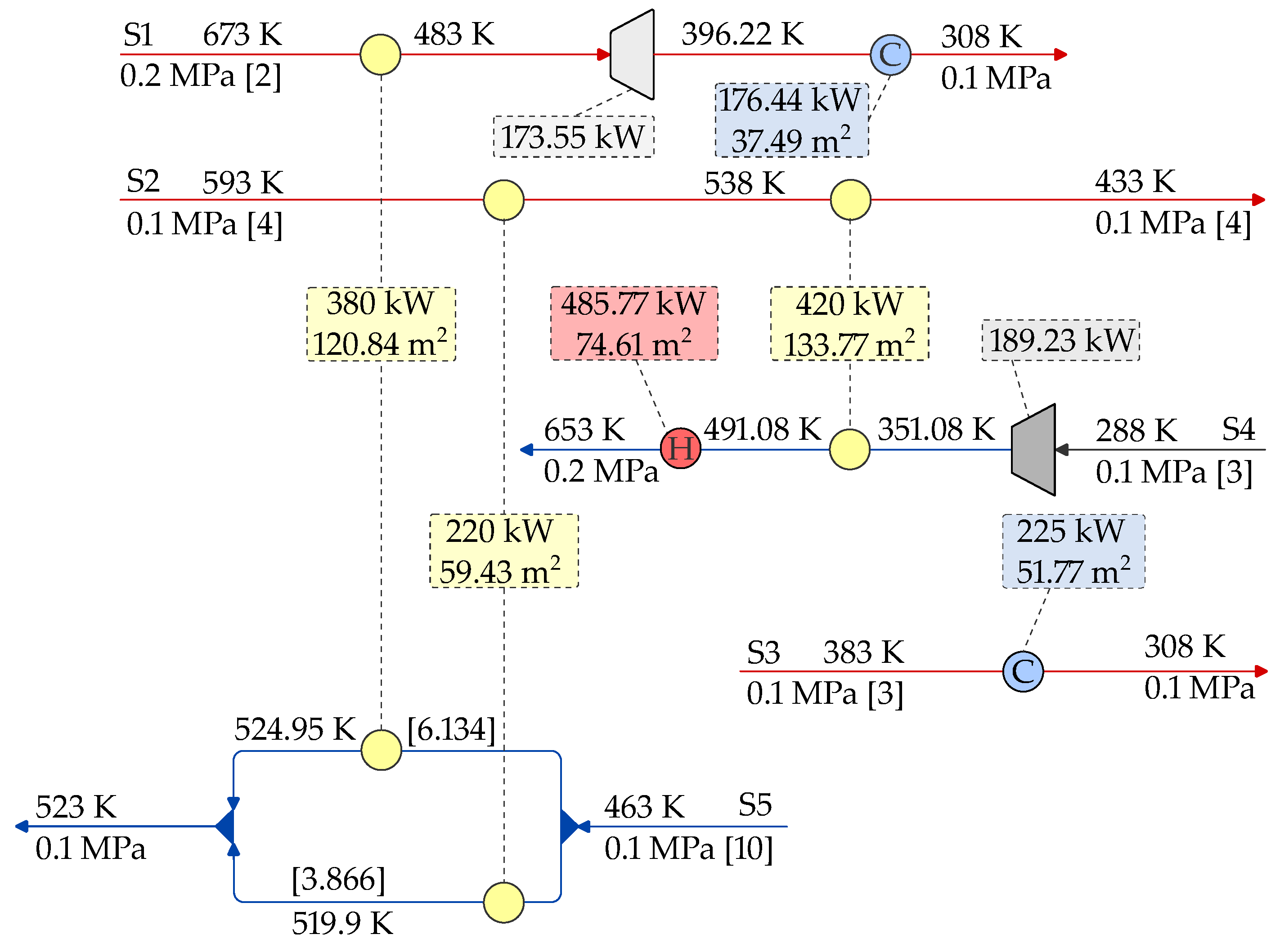
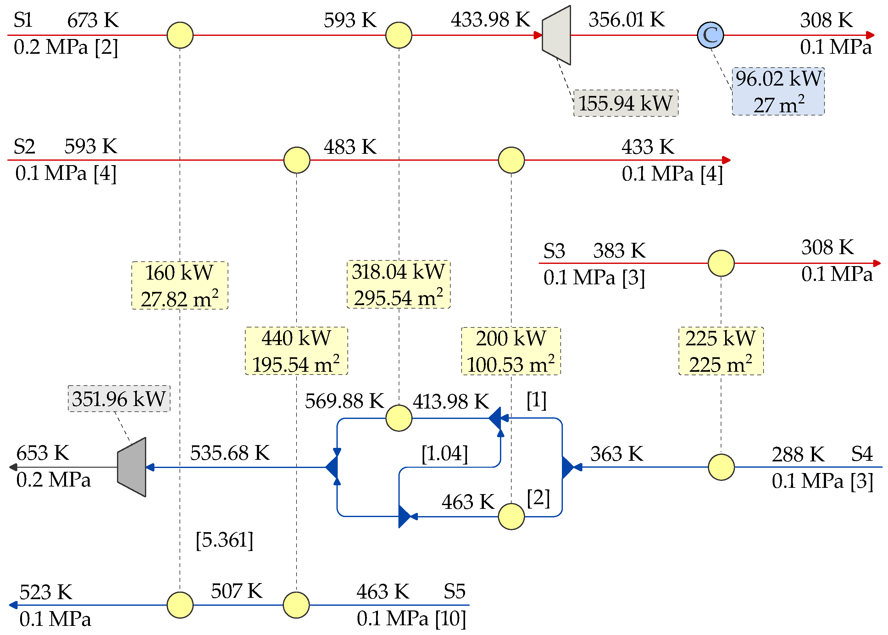
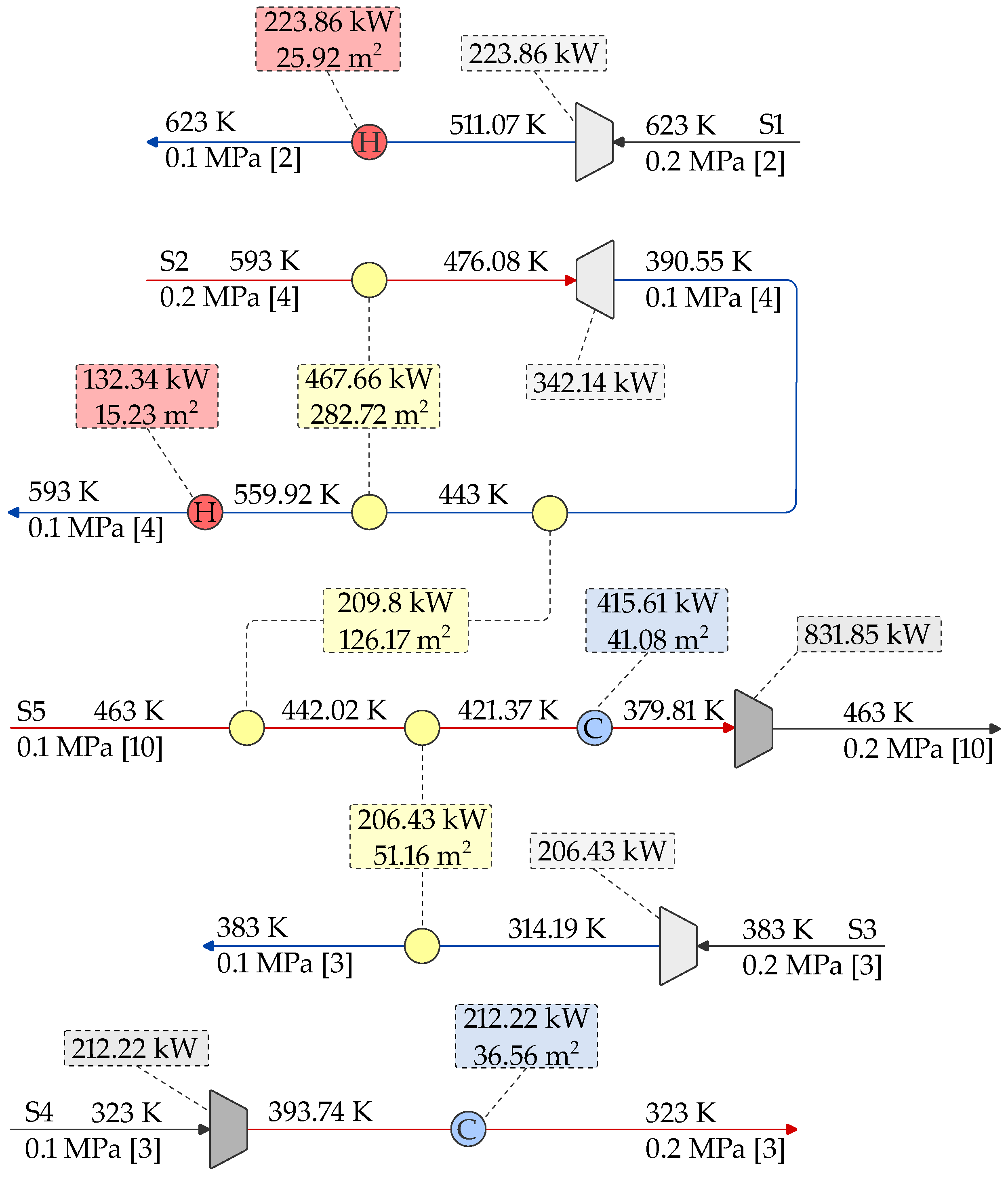
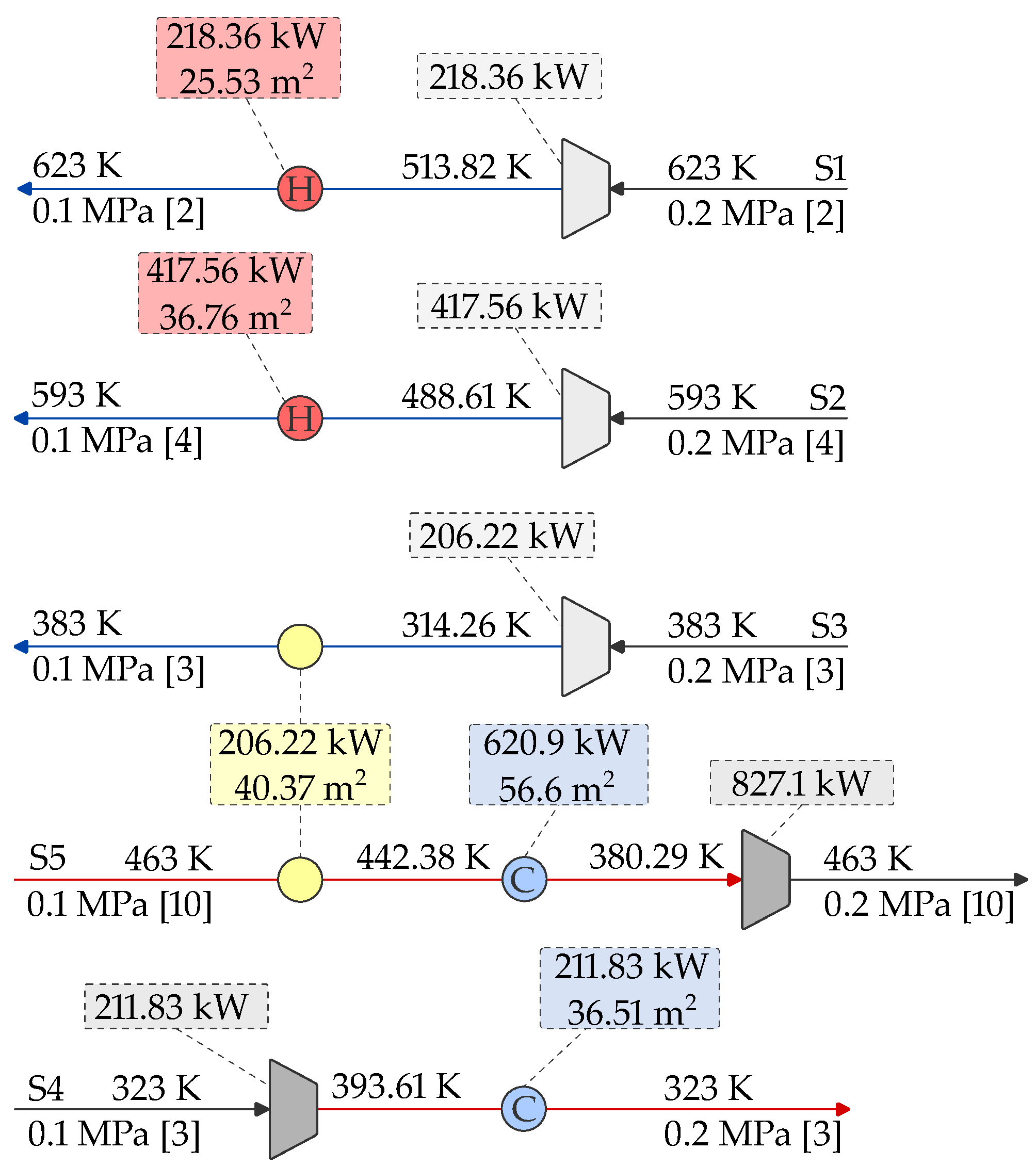
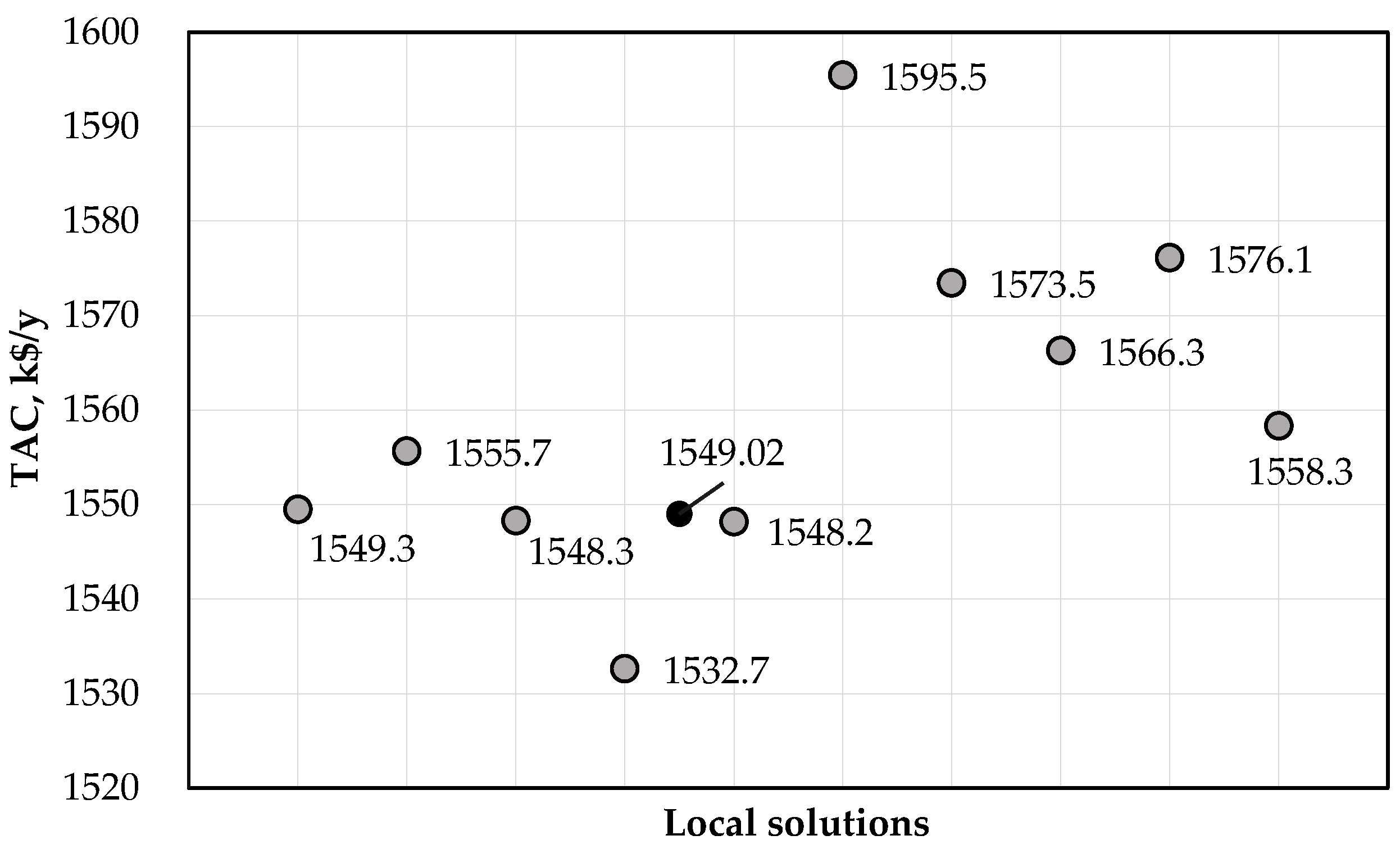
4.4. Example 4
4.5. Model Statistics
5. Conclusions
Author Contributions
Funding
Institutional Review Board Statement
Informed Consent Statement
Data Availability Statement
Acknowledgments
Conflicts of Interest
Abbreviations
| CAPEX | Capital Expenditures |
| COMP | Compressor |
| EMAT | Exchanger Minimum Approach Temperature |
| EXP | Expander |
| GAMS | General Algebraic Modeling System |
| GDP | Generalised Disjunctive Programming |
| HE | Heat Exchanger |
| HEN | Heat Exchanger Network |
| HRAT | Heat Recovery Approach Temperature |
| MINLP | Mixed Integer Nonlinear Programming |
| MP | Mathematical Programming |
| NLP | Nonlinear Programming |
| OPEX | Operational Expenditures |
| PA | Pinch Analysis |
| STHE | Shell and Tube Heat Exchangers |
| TAC | Total Annualized Cost |
| WHI | Work and Heat Integration |
| WHEN | Work and Heat Exchange Network |
| Indices | |
| i | Hot stream |
| j | Cold stream |
| k | Pressure change stage |
| s | Process stream |
| Sets | |
| K | Pressure change stages |
| S | Process streams |
| Subscripts/Superscripts | |
| Bypass | |
| Cooler | |
| Compressor | |
| Consumed | |
| Cold stream/Cold supply | |
| Cold target | |
| Cold utility | |
| Exchanger’s hot stream | |
| Exchanger’s cold stream | |
| Exchanger | |
| Expander | |
| Heater | |
| Hot stream/Hot supply | |
| Hot target | |
| Hot utility | |
| Inter-stage cooling | |
| Ideal | |
| Inter-stage heating | |
| Inlet | |
| Mixer | |
| Maximum | |
| Outlet | |
| Produced | |
| Upper bound | |
| Expansion valve | |
| Parameters | |
| a | Fixed cost for equipment, $ |
| Equipment investment annualization factor, 1/y | |
| b | Variable cost coefficient for equipment, $/attribute |
| BINT | Binary parameter denoting existence of bypass, |
| Cold utility cost, $/kWy | |
| Hot utility cost, $/kWy | |
| Electricity cost, $/kWy | |
| CINT | Binary parameter denoting existence of compression stages, |
| Depreciation period for investment, y | |
| EINT | Binary parameter denoting existence of expansion stages, |
| Bare module factor, | |
| h | Individual heat transfer coefficient, kW/(m2K) |
| Interest rate for investment, %/100 | |
| n | Cost exponent for equipment |
| Isentropic expansion/compression coefficient, | |
| Joule–Thompson expansion coefficient, K/MPa | |
| Isentropic efficiency of compressor/expander, | |
| Process stream s supply temperature, K | |
| Process stream s target temperature, K | |
| Process stream s supply pressure, MPa | |
| Process stream s target pressure, MPa | |
| Upper bound for temperature driving force, K | |
| Continuous variables | |
| A | Heat exchange area, m2 |
| Heat capacity flow rate, kW/K | |
| T | Temperature, K |
| p | Pressure, MPa |
| q | Heat load, kW |
| Temperature difference at hot end of heat exchanger, K | |
| Temperature difference at cold end of heat exchanger, K | |
| Binary variables | |
| z | Existence of equipment, - |
Appendix A
Appendix A.1. Identification of Streams
Appendix A.2. Additional Constraints

References
- Klemeš, J.J.; Kravanja, Z. Forty years of Heat Integration: Pinch Analysis (PA) and Mathematical Programming (MP). Curr. Opin. Chem. Eng. 2013, 2, 461–474. [Google Scholar] [CrossRef]
- Fu, C.; Vikse, M.; Gundersen, T. Work and heat integration: An emerging research area. Energy 2018, 158, 796–806. [Google Scholar] [CrossRef]
- Aspelund, A.; Berstad, D.O.; Gundersen, T. An Extended Pinch Analysis and Design procedure utilizing pressure based exergy for subambient cooling. Appl. Therm. Eng. 2007, 27, 2633–2649. [Google Scholar] [CrossRef]
- Fu, C.; Gundersen, T. Integrating compressors into heat exchanger networks above ambient temperature. AIChE J. 2015, 61, 3770–3785. [Google Scholar] [CrossRef]
- Fu, C.; Gundersen, T. Integrating expanders into heat exchanger networks above ambient temperature. AIChE J. 2015, 61, 3404–3422. [Google Scholar] [CrossRef]
- Fu, C.; Wang, X.; Gundersen, T. The importance of thermodynamic insight in Work and Heat Exchange Network Design. Chem. Eng. Trans. 2020, 81, 127–132. [Google Scholar] [CrossRef]
- Wechsung, A.; Aspelund, A.; Gundersen, T.; Barton, P.I. Synthesis of heat exchanger networks at subambient conditions with compression and expansion of process streams. AIChE J. 2011, 57, 2090–2108. [Google Scholar] [CrossRef]
- Huang, K.; Karimi, I.A. Work-heat exchanger network synthesis (WHENS). Energy 2016, 113, 1006–1017. [Google Scholar] [CrossRef]
- Huang, K.F.; Al-mutairi, E.M.; Karimi, I.A. Heat exchanger network synthesis using a stagewise superstructure with non-isothermal mixing. Chem. Eng. Sci. 2012, 73, 30–43. [Google Scholar] [CrossRef]
- Onishi, V.C.; Ravagnani, M.A.; Caballero, J.A. Simultaneous synthesis of work exchange networks with heat integration. Chem. Eng. Sci. 2014, 112, 87–107. [Google Scholar] [CrossRef]
- Yee, T.F.; Grossmann, I.E. Simultaneous optimization models for heat integration—II. Heat exchanger network synthesis. Comput. Chem. Eng. 1990, 14, 1165–1184. [Google Scholar] [CrossRef]
- Onishi, V.C.; Ravagnani, M.A.; Caballero, J.A. MINLP Model for the Synthesis of Heat Exchanger Networks with Handling Pressure of Process Streams. Comput. Aided Chem. Eng. 2014, 33, 163–168. [Google Scholar] [CrossRef]
- Pavão, L.V.; Costa, C.B.; Ravagnani, M.A. A new framework for work and heat exchange network synthesis and optimization. Energy Convers. Manag. 2019, 183, 617–632. [Google Scholar] [CrossRef]
- Onishi, V.C.; Ravagnani, M.A.S.S.; Caballero, J.A. Simultaneous synthesis of heat exchanger networks with pressure recovery: Optimal integration between heat and work. AIChE J. 2014, 60, 893–908. [Google Scholar] [CrossRef]
- Pavão, L.V.; Costa, C.B.B.; Ravagnani, M.A.S.S. An Enhanced Stage-wise Superstructure for Heat Exchanger Networks Synthesis with New Options for Heaters and Coolers Placement. Ind. Eng. Chem. Res. 2018, 57, 2560–2573. [Google Scholar] [CrossRef]
- Pavão, L.V.; Caballero, J.A.; Ravagnani, M.A.; Costa, C.B. An extended method for work and heat integration considering practical operating constraints. Energy Convers. Manag. 2020, 206, 112469. [Google Scholar] [CrossRef]
- Nair, S.K.; Nagesh Rao, H.; Karimi, I.A. Framework for work-heat exchange network synthesis (WHENS). AIChE J. 2018, 64, 2472–2485. [Google Scholar] [CrossRef]
- Onishi, V.C.; Quirante, N.; Ravagnani, M.A.; Caballero, J.A. Optimal synthesis of work and heat exchangers networks considering unclassified process streams at sub and above-ambient conditions. Appl. Energy 2018, 224, 567–581. [Google Scholar] [CrossRef]
- Duran, M.A.; Grossmann, I.E. Simultaneous optimization and heat integration of chemical processes. Aiche J. 1986, 32, 123–138. [Google Scholar] [CrossRef]
- Quirante, N.; Caballero, J.A.; Grossmann, I.E. A novel disjunctive model for the simultaneous optimization and heat integration. Comput. Chem. Eng. 2017, 96, 149–168. [Google Scholar] [CrossRef]
- Li, J.; Demirel, S.E.; Hasan, M.M.F. Building Block-Based Synthesis and Intensification of Work-Heat Exchanger Networks (WHENS). Processes 2019, 7, 23. [Google Scholar] [CrossRef]
- Pavão, L.V.; Caballero, J.A.; Ravagnani, M.A.; Costa, C.B. A pinch-based method for defining pressure manipulation routes in work and heat exchange networks. Renew. Sustain. Energy Rev. 2020, 131, 109989. [Google Scholar] [CrossRef]
- Linnhoff, B.; Ahmad, S. Cost optimum heat exchanger networks—1. Minimum energy and capital using simple models for capital cost. Comput. Chem. Eng. 1990, 14, 729–750. [Google Scholar] [CrossRef]
- Yu, H.; Vikse, M.; Anantharaman, R.; Gundersen, T. Model reformulations for Work and Heat Exchange Network (WHEN) synthesis problems. Comput. Chem. Eng. 2019, 125, 89–97. [Google Scholar] [CrossRef]
- Lin, Q.; Liao, Z.; Sun, J.; Jiang, B.; Wang, J.; Yang, Y. Targeting and Design of Work and Heat Exchange Networks. Ind. Eng. Chem. Res. 2020, 59, 12471–12486. [Google Scholar] [CrossRef]
- Lin, Q.; Chang, C.; Liao, Z.; Sun, J.; Jiang, B.; Wang, J.; Yang, Y. Efficient Strategy for the Synthesis of Work and Heat Exchange Networks. Ind. Eng. Chem. Res. 2021, 60, 1756–1773. [Google Scholar] [CrossRef]
- Lin, Q.; Liao, Z.; Bagajewicz, M.J. Globally optimal design of Minimal WHEN systems using enumeration. AIChE J. 2023, 69, e17878. [Google Scholar] [CrossRef]
- Yang, R.; Zhuang, Y.; Zhang, L.; Du, J.; Shen, S. A thermo-economic multi-objective optimization model for simultaneous synthesis of heat exchanger networks including compressors. Chem. Eng. Res. Des. 2020, 153, 120–135. [Google Scholar] [CrossRef]
- Zhuang, Y.; Yang, R.; Zhang, L.; Du, J.; Shen, S. Simultaneous synthesis of sub and above-ambient heat exchanger networks including expansion process based on an enhanced superstructure model. Chin. J. Chem. Eng. 2020, 28, 1344–1356. [Google Scholar] [CrossRef]
- Zhuang, Y.; Xing, Y.; Zhang, L.; Liu, L.; Du, J.; Shen, S. An enhanced superstructure-based model for work-integrated heat exchange network considering inter-stage multiple utilities optimization. Comput. Chem. Eng. 2021, 152, 107388. [Google Scholar] [CrossRef]
- Braccia, L.; Luppi, P.; Vallarella, A.J.; Zumoffen, D. Generalized simultaneous optimization model for synthesis of heat and work exchange networks. Comput. Chem. Eng. 2022, 168, 108036. [Google Scholar] [CrossRef]
- Yu, H.; Fu, C.; Gundersen, T. Work Exchange Networks (WENs) and Work and Heat Exchange Networks (WHENs): A Review of the Current State of the Art. Ind. Eng. Chem. Res. 2020, 59, 507–525. [Google Scholar] [CrossRef]
- Floudas, C.A.; Ciric, A.R.; Grossmann, I.E. Automatic synthesis of optimum heat exchanger network configurations. AIChE J. 1986, 32, 276–290. [Google Scholar] [CrossRef]
- Yu, H.; Fu, C.; Vikse, M.; He, C.; Gundersen, T. Identifying optimal thermodynamic paths in work and heat exchange network synthesis. AIChE J. 2019, 65, 549–561. [Google Scholar] [CrossRef]
- Biegler, L.T.; Grossmann, I.E.; Westerberg, A.W. Systematic Methods for Chemical Process Design; Prentice Hall, Inc., NJ, USA, 1997.
- Chen, J. Comments on improvements on a replacement for the logarithmic mean. Chem. Eng. Sci. 1987, 42, 2488–2489. [Google Scholar] [CrossRef]
- Chen, J. Logarithmic mean: Chen’s approximation or explicit solution? Comput. Chem. Eng. 2019, 120, 1–3. [Google Scholar] [CrossRef]
- Smith, R. Chemical Process Design and Integration, 2nd ed.; John Wiley & Sons, Inc.: Chichester, UK, 2016. [Google Scholar]
- GAMS Development Corporation. General Algebraic Modeling System (GAMS), Release 36.1.0; GAMS Development Corporation: Fairfax, VA, USA, 2022.
- Systat Software Inc. SigmaPlot, v 14; Systat Software Inc.: San Jose, CA, USA, 2017.
- Seider, W.; Seader, J.; Lewin, D. Product and Process Design Principles: Synthesis, Analysis and Evaluation, 3rd ed.; John Wiley & Sons, Inc.: Hoboken, NJ, USA, 2008. [Google Scholar]
- Peters, M.; Timmerhaus, K.; West, R. Plant Design and Economics for Chemical Engineers, 4th ed.; McGraw-Hill Chemical Engineering Series; McGraw-Hill, Inc.: New York, NY, USA, 2003. [Google Scholar]
- Couper, J.R.; Penney, W.R.; Fair, J.R.; Walas, S.M. 21—Costs of Individual Equipment. In Chemical Process Equipment, 3rd ed.; Couper, J.R., Penney, W.R., Fair, J.R., Walas, S.M., Eds.; Butterworth-Heinemann: Boston, MA, USA, 2012; pp. 731–741. [Google Scholar] [CrossRef]
- Woods, D.R. Appendix D: Capital Cost Guidelines. In Rules of Thumb in Engineering Practice; Wiley-VCH Verlag GmbH & Co. KGaA: Weinheim, Germany, 2007; pp. 376–436. [Google Scholar] [CrossRef]
- Towler, G.; Sinnott, R. Chapter 7—Capital cost estimating. In Chemical Engineering Design, 3rd ed.; Towler, G., Sinnott, R., Eds.; Butterworth-Heinemann: Cambridge, MA, USA, 2022; pp. 239–278. [Google Scholar] [CrossRef]
- Turton, R.; Bailie, R.C.; Whiting, W.B.; Shaeiwitz, J.A.; Bhattacharyya, D. Analysis, Synthesis, and Design of Chemical Processes; Prentice-Hall International Series in Engineering; Prentice Hall: Upper Saddle River, NJ, USA, 2012. [Google Scholar]
- Shah, N.M.; Rangaiah, G.P.; Hoadley, A.F. Multi-objective optimization of multi-stage gas-phase refrigeration systems. In Multi-Objective Optimization: Techniques and Application in Chemical Engineering; World Scientific Publishing Co. Pte. Ltd.: Singapore, 2017; pp. 247–290. [Google Scholar]
- Fu, C.; Gundersen, T. Correct integration of compressors and expanders in above ambient heat exchanger networks. Energy 2016, 116, 1282–1293. [Google Scholar] [CrossRef]


| Parameter | Unit | Examples 1–3 | Example 4 |
|---|---|---|---|
| Heating utility cost | k$/kWy | 0.377 | 0.337 |
| Cooling utility cost | k$/kWy | 0.1 | 0.1 |
| Electricity cost (consumed) | k$/KWy | 0.45505 | 0.45505 |
| Electricity cost (produced) | k$/KWy | 0.45505 | 0.36403 |
| Joule–Thompson coefficient of expansion | K/MPa | 1.961 | - |
| Isentropic efficiency | - | 1 | 1 |
| Reference | S Range | Equipment | a | b | n | R2 |
|---|---|---|---|---|---|---|
| Seider et al. [41] | 149–22,371 | COMP | - | 4.0422 | 0.8 | 1 |
| 15–3728 | EXP | - | 1.1097 | 0.81 | 1 | |
| 4–1115 | STHE | 23.0784 | 0.1165 | 1 | 0.9989 | |
| 20.7139 | 0.208 | 0.9166 | 1 | |||
| Peters et al. [42] | 75–3000 | COMP | - | 1.8337 | 0.9435 | 1 |
| 100–3000 | EXP | - | 6.9313 | 0.5889 | 1 | |
| 10–1000 | STHE | 12.342 | 0.17 | 1 | 0.9991 | |
| 9.0307 | 0.2889 | 0.9239 | 0.9997 | |||
| Couper et al. [43] | 149–22,371 | COMP | - | 19.235 | 0.62 | 1 |
| 15–3728 | EXP | - | 0.9731 | 0.81 | 1 | |
| 14–1115 | STHE | 7.0232 | 0.2479 | 1 | 0.9996 | |
| 9.5624 | 0.1785 | 1.0469 | 0.9999 | |||
| Woods [44] | 2–4000 | COMP | - | 2.198 | 0.9 | 1 |
| 746–22,371 | EXP | - | 1.7929 | 0.8 | 1 | |
| 20–1150 | STHE | - | 2.8628 | 0.65 | 1 | |
| Towler and Sinnott [45] | 75–30,000 | COMP | 888.122 | 30.625 | 0.6 | 1 |
| 1000–15,000 | EXP * | 1026.8 | 0.1968 | 1 | 1 | |
| 10–1000 | STHE | 49 | 0.1072 | 1.2 | 1 | |
| Turton [46] | 450–3000 | COMP | - | 4.2380 | 0.71 | 0.9993 |
| 100–3000 | EXP | −2140.823 | 1641.81 | 0.0712 | 0.9983 | |
| 20–1000 | STHE | 34.1951 | 0.0876 | 1.1532 | 0.9999 |
| Stream | (K) | (K) | (kW/K) | (MPa) | (MPa) | h (kW/m2K) |
|---|---|---|---|---|---|---|
| S1 | 637 | 333 | 2 | 0.1 | 0.1 | 0.1 |
| S2 | 288 | 523 | 1 | 0.1 | 0.3 | 0.1 |
| S3 | 472 | 543 | 4 | 0.1 | 0.1 | 0.1 |
| HU | 673 | 673 | - | - | - | 1 |
| CU | 288 | 288 | - | - | - | 1 |
| Indicator | Unit | Seider et al. [41] | Couper et al. [43] | Peters et al. [42] | Towler and Sinnott [45] |
|---|---|---|---|---|---|
| No. of HEs | - | 5 | 5 | 5 | 5 |
| No. of COMP | - | 1 | 1 | 1 | 1 |
| HU demand | kW | 235.587 | 235.587 | 235.587 | 235.587 |
| CU demand | kW | 135 | 135 | 135 | 135 |
| Compression work | kW | 174.41 | 174.41 | 174.41 | 174.41 |
| Total CAPEX | k$ | 407.928 | 598.092 | 363.073 | 1908.525 |
| CAPEX | k$/y | 60.685 | 89.133 | 54.109 | 284.427 |
| OPEX | k$/y | 181.683 | 181.683 | 181.683 | 181.683 |
| TAC | k$/y | 242.368 | 270.816 | 235.792 | 466.110 |
| Indicator | Unit | Fu and Gundersen [4] Case A | Fu and Gundersen [4] Case B | This Work |
|---|---|---|---|---|
| HU demand | kW | 410 | 235.5 | 235.59 |
| CU demand | kW | 241.3 | 135.0 | 135.0 |
| Compression work | kW | 106.3 | 174.5 | 174.41 |
| Exergy consumption | kW | 340.8 | 309.2 | 309.2 |
| Total CAPEX | k$ | 1742.0 | 1908.73 | 1908.52 |
| CAPEX | k$/y | 259.610 | 284.457 | 284.427 |
| OPEX | k$/y | 227.073 | 181.691 | 181.683 |
| TAC | k$/y | 486.682 | 466.148 | 466.110 |
| Indicator | Unit | Electricity Cost (k$/kWy) | ||
|---|---|---|---|---|
| 0.2275 | 0.45505 | 0.6826 | ||
| No. of HEs | - | 5 | 5 | 4 |
| HU demand | kW | 235.59 | 235.59 | 410 |
| CU demand | kW | 135.0 | 135.0 | 241.2 |
| Compression work | kW | 174.41 | 174.41 | 106.2 |
| Exergy consumption | kW | 309.2 | 309.2 | 340.74 |
| Total CAPEX | k$ | 1908.52 | 1908.52 | 1681.17 |
| CAPEX | k$/y | 284.427 | 284.427 | 250.543 |
| OPEX | k$/y | 141.995 | 181.683 | 251.18 |
| TAC | k$/y | 426.422 | 466.110 | 501.723 |
| Stream | (K) | (K) | (kW/K) | (MPa) | (MPa) | h (kW/m2K) |
|---|---|---|---|---|---|---|
| S1 | 673 | 333 | 3 | 0.3 | 0.1 | 0.1 |
| S2 | 603 | 353 | 9 | 0.1 | 0.1 | 0.1 |
| S3 | 288 | 493 | 6 | 0.1 | 0.1 | 0.1 |
| S4 | 413 | 653 | 8 | 0.1 | 0.1 | 0.1 |
| HU | 673 | 673 | - | - | - | 1 |
| CU | 288 | 288 | - | - | - | 1 |
| Indicator | Unit | Annualization Factor | |||||
|---|---|---|---|---|---|---|---|
| 0.08 | 0.1 | 0.2 | 0.3 | 0.5 | 1 | ||
| No. of HE | 9 | 9 | 7 | 7 | 6 | 6 | |
| HU demand | kW | 350 | 350 | 350 | 366.55 | 401.46 | 491.70 |
| CU demand | kW | 67.07 | 67.14 | 81.44 | 98.99 | 153.09 | 243.33 |
| Expansion work | kW | 402.93 | 402.86 | 388.56 | 387.55 | 368.37 | 368.37 |
| Total CAPEX | k$ | 644.88 | 643.857 | 598.897 | 567.351 | 493.432 | 435.125 |
| CAPEX | k$/y | 51.59 | 64.386 | 119.779 | 170.205 | 246.716 | 435.125 |
| OPEX | k$/y | −44.696 | −44.658 | −36.721 | −28.268 | −0.965 | 42.079 |
| TAC | k$/y | 6.894 | 19.727 | 83.058 | 141.937 | 245.751 | 477.204 |
| Indicator | Unit | Fu and Gundersen [5] Case A | Fu and Gundersen [5] Case B | Fu and Gundersen [5] Case C | This Work |
|---|---|---|---|---|---|
| No. of HEs | - | 7 | 8 | 9 | 7 |
| No. of EXP | - | 1 | 1 | 2 | 1 |
| HU demand | kW | 694 | 637.5 | 350 | 350 |
| CU demand | kW | 270 | 270 | 63.5 | 67.14 |
| Expansion work | kW | 543.9 | 487.5 | 406.6 | 402.86 |
| Exergy consumption | kW | −147.0 | −122.9 | −206.4 | −188.34 |
| Total CAPEX | k$ | 651.771 | 599.452 | 772.952 | 643.857 |
| CAPEX | k$/y | 65.177 | 59.945 | 77.295 | 64.386 |
| OPEX | k$/y | 41.131 | 45.496 | −46.727 | −44.658 |
| TAC | k$/y | 106.308 | 105.441 | 30.568 | 19.727 |
| Stream | (K) | (K) | (kW/K) | (MPa) | (MPa) | h (kW/m2K) |
|---|---|---|---|---|---|---|
| S1 | 673 | 308 | 2 | 0.2 | 0.1 | 0.1 |
| S2 | 593 | 433 | 4 | 0.1 | 0.1 | 0.1 |
| S3 | 383 | 308 | 3 | 0.1 | 0.1 | 0.1 |
| S4 | 288 | 653 | 3 | 0.1 | 0.2 | 0.1 |
| S5 | 463 | 523 | 10 | 0.1 | 0.1 | 0.1 |
| HU | 673 | 673 | - | - | - | 1 |
| CU | 288 | 288 | - | - | - | 1 |
| Indicator | Unit | Fu and Gundersen [48] Case I | Fu and Gundersen [48] Case II | Fu and Gundersen [48] Case III | This Work |
|---|---|---|---|---|---|
| No. of HEs | - | 8 | 8 | 11 | 6 |
| No. of EXP | - | 1 | 1 | 2 | 1 |
| No. of COMP | - | 1 | 1 | 2 | 1 |
| Hot utility demand | kW | 591.8 | 119.4 | 37.6 | 485.71 |
| Cold utility demand | kW | 439.4 | 150 | 91.7 | 225 |
| Compression work | kW | 189.3 | 304.2 | 312.4 | 189.23 |
| Expansion work | kW | 241.8 | 173.6 | 158.3 | 173.55 |
| Exergy consumption | kW | 286.0 | 198.9 | 175.6 | 293.6 |
| Total CAPEX | k$ | 10,037.51 | 10,824.71 | 18,246.25 | 9574.04 |
| CAPEX | k$/y | 1806.75 | 1948.45 | 3284.32 | 1723.33 |
| OPEX | k$/y | 243.120 | 119.445 | 93.45 | 230.392 |
| TAC | k$/y | 2049.87 | 2067.89 | 3377.794 | 1953.742 |
| Stream | (K) | (K) | (kW/K) | (MPa) | (MPa) | h (kW/m2K) |
|---|---|---|---|---|---|---|
| S1 | 623 | 623 | 2 | 0.2 | 0.1 | 0.1 |
| S2 | 593 | 593 | 4 | 0.2 | 0.1 | 0.1 |
| S3 | 383 | 383 | 3 | 0.2 | 0.1 | 0.1 |
| S4 | 323 | 323 | 3 | 0.1 | 0.2 | 0.1 |
| S5 | 463 | 463 | 10 | 0.1 | 0.2 | 0.1 |
| HU | 673 | 673 | - | - | - | 1 |
| CU | 288 | 288 | - | - | - | 1 |
| Reference | Equipment | a | b | n |
|---|---|---|---|---|
| Lin et al. [27] | COMP | - | 51,104.85 | 0.62 |
| EXP | - | 2585.47 | 0.81 | |
| STHE | 99,163 | 250.9 | 1.1577 | |
| Cost Parameter | ||||
| $/kWy | 455.05 | 364.03 | 337 | 100 |
| Indicator | Unit | Yu et al. [34] | Lin et al. [27] | This Work |
|---|---|---|---|---|
| Number of COMP and EXP | - | 7 | 5 | 5 |
| Number of HE units | - | 13 | 5 | 10 |
| Hot utility demand | kW | 40 | 635.92 | 356.2 |
| Cold utility demand | kW | 342.7 | 832.73 | 627.83 |
| Compression work | kW | 1127.3 | 1038.93 | 1044.07 |
| Expansion work | kW | 827.4 | 842.14 | 772.43 |
| Total CAPEX | k$ | 9719.198 | 6029.103 | 6421.778 |
| CAPEX | k$/y | 1749.455 | 1085.239 | 1155.92 |
| OPEX | k$/y | 259.528 | 463.79 | 376.749 |
| TAC | k$/y | 2008.983 | 1549.028 | 1532.658 |
| Example 1 | Example 2 | Example 3 | Example 4 | |
|---|---|---|---|---|
| Step 1—NLP | ||||
| No. of equations | 120 | 157 | 210 | 229 |
| No. of continuous variables | 114 | 153 | 202 | 221 |
| CPU time, s | 3.8 | 24 | 0.1 | 37.9 |
| Step 2—MINLP | ||||
| No. of equations | 353 | 486 | 773 | 713 |
| No. of continuous variables | 323 | 466 | 866 | 744 |
| No. of discrete variables | 23 | 31 | 50 | 45 |
| CPU time, s | 3.3 | 26.9 | 546 | 221 |
Disclaimer/Publisher’s Note: The statements, opinions and data contained in all publications are solely those of the individual author(s) and contributor(s) and not of MDPI and/or the editor(s). MDPI and/or the editor(s) disclaim responsibility for any injury to people or property resulting from any ideas, methods, instructions or products referred to in the content. |
© 2024 by the authors. Licensee MDPI, Basel, Switzerland. This article is an open access article distributed under the terms and conditions of the Creative Commons Attribution (CC BY) license (https://creativecommons.org/licenses/by/4.0/).
Share and Cite
Ibrić, N.; Fu, C.; Gundersen, T. Simultaneous Optimization of Work and Heat Exchange Networks. Energies 2024, 17, 1753. https://doi.org/10.3390/en17071753
Ibrić N, Fu C, Gundersen T. Simultaneous Optimization of Work and Heat Exchange Networks. Energies. 2024; 17(7):1753. https://doi.org/10.3390/en17071753
Chicago/Turabian StyleIbrić, Nidret, Chao Fu, and Truls Gundersen. 2024. "Simultaneous Optimization of Work and Heat Exchange Networks" Energies 17, no. 7: 1753. https://doi.org/10.3390/en17071753