Advanced Flame front Detection in Combustion Processes Using Autoencoder Approach

Abstract

This research explores the detection of flame front evolution in spark-ignition engines using an innovative neural network, the autoencoder. High-speed camera images from an optical access engine were analyzed under different air excess coefficient λ conditions to evaluate the autoencoder’s performance. This study compared this new approach (AE) with an established method used by the same research group (BR) across multiple combustion cycles. Results revealed that the AE method outperformed the BR in accurately identifying flame pixels and significantly reducing overestimations outside the flame boundary. AE exhibited higher sensitivity levels, indicating its superior ability to identify pixels and minimize errors compared to the BR method. Additionally, AE’s accuracy in representing combustion evolution was notably improved, offering a more detailed depiction of the process. AE’s strength lies in its independence from specific threshold searches, a requirement in the BR method. By relying on learned representations within its latent space, AE eliminates laborious threshold exploration, ensuring reliability and reducing workload pressures. Comparative analyses consistently confirmed AE’s superior performance in accurately reproducing and delineating combustion evolution compared to BR. This study highlights AE’s potential as a promising technique for precise flame front detection in combustion processes. Its ability to autonomously extract features, minimize errors, and enhance overall accuracy signifies a significant step forward in analyzing flame fronts. AE’s reliability, reduced need for manual intervention, and adaptability across various conditions suggest a promising future for improving combustion analysis techniques in spark-ignition engines with optical access.

1. Introduction

In recent decades, advancements in both experimental and computational research have facilitated a comprehensive examination of the fundamental physical processes taking place within spark-ignition (SI) internal combustion engines (ICEs) [1,2,3]. In the field of ICE, researchers often rely on single-cylinder optical access engines to perform a morphological analysis of the flame front evolution [4,5]. 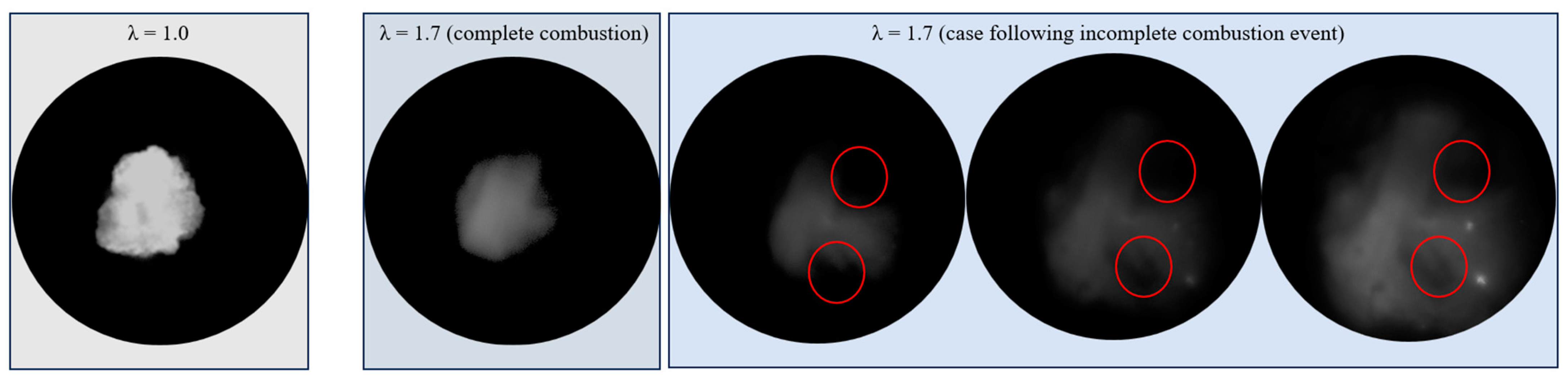The identification of kernel formations holds significant importance in assessing the ability of an igniter to guarantee strong combustion events [6], particularly in critical operating conditions such as lean–ultra-lean fuel mixtures [7]. These conditions, characterized by low luminosity, notably hinder the recognition of combustion evolution, particularly in capturing the early stages of flame development. Moreover, the opacity of the images, caused by the accumulation of residues on the piston head together with reflections from objects inside the combustion chamber, complicates the observation process, intensifying the haze effect with each cycle [8]. The challenges in successfully detecting the physical aspects of flame front evolution therefore require robust and advanced techniques. At present, Machine Learning (ML) sees growing utilization in controlling engine parameters [9], categorizing images [10], eliminating background noise [11], and identifying objects and edges [12]. Concerning the latter, the literature shows the promising results of deep learning algorithms based on a Convolutional Neural Network (CNN) [13,14].

In previous works of the same research group [15], ML algorithms with CNN structures were employed to detect the flame front evolving in a single-cylinder optical access engine and the corresponding performance compared with the ones obtained through the utilization of a semi-automatic algorithm proposed by Shawal et al. [16] and used as a base reference. The results show that the proposed methods identify some combustions, initially marked as misfires or anomalies by the base reference method as valid. This shift allows for a closer examination of the igniter’s performance during the early kernel formation. It creates a strong match between an analysis using indicators and visual imaging. Additionally, metric parameters confirm superiority in accuracy, sensitivity, and specificity [17] on average of the proposed algorithms, making it more suitable for analyzing ultra-lean combustion, a focal point in automotive research. The algorithms’ automated threshold estimation enhances detailed flame analyses, showcasing their potential in improving combustion analysis techniques. However, the segmentation and labeling process needed for training the abovementioned models required human intervention. This manual effort is time-consuming and introduces subjectivity, potentially affecting the model’s ability to generalize across different datasets or conditions. Moreover, the training of such models demands substantial computational power, particularly when handling a large volume of images or high-resolution data. This necessity for significant computing resources can be costly and time-consuming. Therefore, exploring the potential of diverse approaches is deemed necessary. Employing an autoencoder-based methodology [18] presents an opportunity to streamline the preprocessing phase, diminishing the reliance on manual segmentation and labeling [19]. 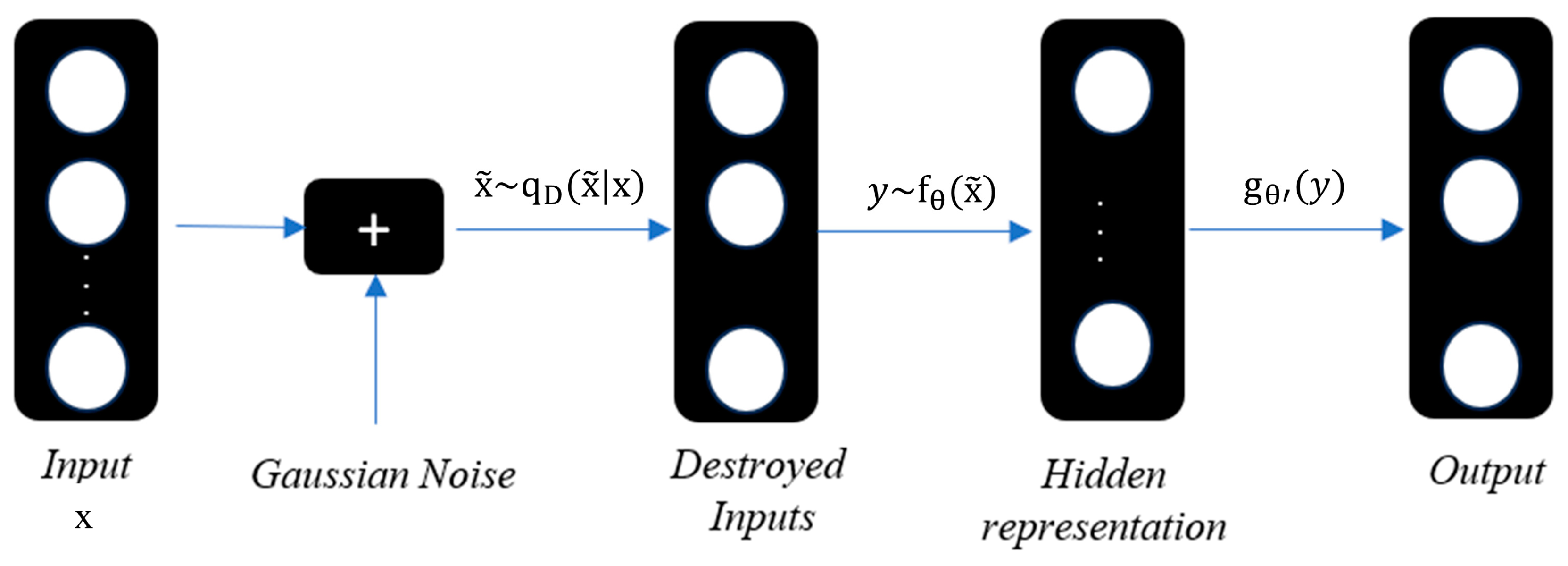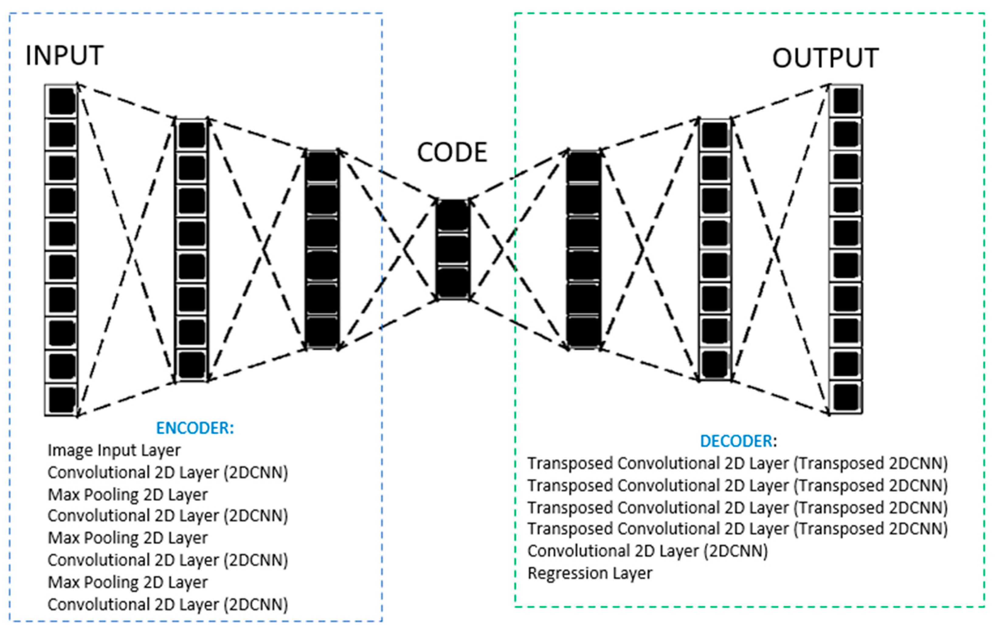By harnessing the autoencoder’s capacity to autonomously extract meaningful features, this approach could mitigate subjectivity, enhance generalizability across diverse datasets, and curtail the computational resources necessitated during training [20]. Delving into this path could reveal a better and more adaptable system for identifying flame fronts in a combustion analysis. An autoencoder is a type of artificial neural network used for unsupervised learning, which consists of an encoder and a decoder [21]. The encoder compresses the input data into a latent space representation, reducing it to its core features. This compressed representation is then decoded by the decoder to reconstruct the original input as accurately as possible. It aims to learn efficient representations of the data by minimizing the reconstruction error between the input and the output [21]. Karimpouli et al. [22] enhanced Digital Rock Physics (DRP) segmentation using a convolutional autoencoder algorithm on 20 Berea sandstone images. Through data augmentation, 20,000 realizations were generated. The extended CNN architecture achieved a 96% categorical accuracy on the test set, surpassing conventional methods that utilize thresholding to define separate stages, making it challenging to automatically differentiate them. Cheng et al. [23] introduced a novel image compression architecture based on a convolutional autoencoder. The design involved a symmetric convolutional autoencoder (CAE) with multiple down-sampling and up-sampling units, replacing conventional transforms. This CAE underwent training using an approximated rate-distortion function to optimize coding efficiency. Additionally, applying a principal component analysis (PCA) to feature maps resulted in a more energy-compact representation, enhancing coding efficiency further. The experiments showcased superior performance, achieving a remarkable 13.7% BD-rate improvement over JPEG2000 on Kodak database images. Posch et al. [24] employed a variational autoencoder (VAE) to create artificial flow fields for engine combustion simulations. The VAE accurately replicated input data and produced 20 sets of fields for simulations. Results indicated a decrease in variability in VAE-generated cycles compared to the original data: original data showed 1.69% and 1.29% variability in peak firing pressure and MFB 50%, while VAE-generated cycles exhibited 0.65% and 0.71%, respectively. The VAE maintained fundamental physics, surpassing traditional methods in preserving flow field properties.

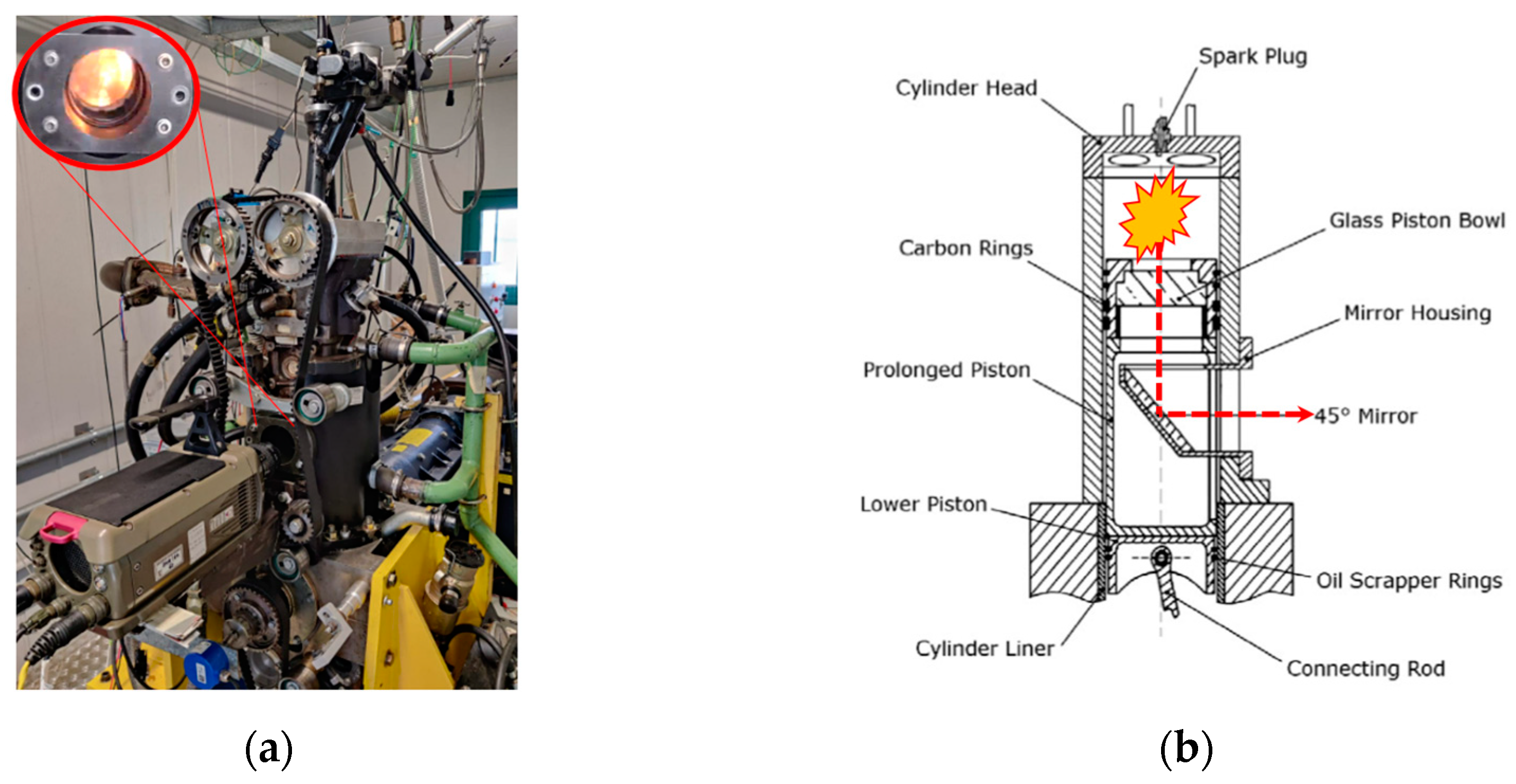
Within this contest, the present work delves into a comprehensive analysis of combustion processes, specifically focusing on the flame front evolution detection of images obtained via a high-speed camera and coming from an optical access engine. This study employs an autoencoder, i.e., an innovative neural network architecture, and operates via unsupervised learning, utilizing an encoder–decoder structure to reconstruct input data, thereby delineating flame fronts. Tests were conducted at 1000 rpm under two different air excess coefficient λ [25] conditions. The initial evaluation of the proposed ANN algorithm’s performance occurred at λ = 1, while subsequent tests explored lower brightness and critical conditions due to quartz fouling risk, at λ = 1.7. The proposed method eliminates noise effectively, leveraging learned representations within its latent space, resulting in enhanced precision and accuracy compared to the method previously established by the same research group [26]. This research conducts an in-depth comparison between these methodologies, evaluating their performance through various quantitative metrics. Sensitivity, specificity, and accuracy metrics were employed to gauge the precision in identifying flame pixels, distinguishing edge and non-edge pixels, and overall performance in delineating combustion evolution. The evaluation involved an analysis of over 63 combustion cycles, leveraging both qualitative and quantitative assessments. Results showcase the superiority of the proposed method over the base-reference approach. The autoencoder architecture [27,28,29,30] (from now on AE) exhibits higher sensitivity levels, indicating its superior capability in accurately identifying pixels outside the flame edge, leading to reduced overestimations if compared to the method used as the base reference (from now on BR). Moreover, AE demonstrates improved accuracy, precisely delineating both edge and non-edge pixels, which significantly enhances the representation of combustion evolution. Notably, the AE method’s robustness and reliability are highlighted by its independence from specific threshold exploration, a requirement in the BR methodology. AE’s automated processing and reliance on learned representations within its latent space eliminate the need for laborious threshold searches, offering enhanced reliability and reduced workload pressures. Furthermore, the comparative analysis with manually obtained binarized images and early flame development assessments consistently affirm AE’s superior performance in accurately reproducing and delineating combustion evolution compared to the established BR method. These findings underscore AE’s potential as a promising methodology for accurate flame front evolution detection in combustion processes.

2. Materials and Methods

2.1. Experimental Setup

The experiments were conducted on a 500-cc single-cylinder research engine with optical accessibility (Figure 1). This engine features four valves, a pent-roof combustion chamber, and a reverse tumble intake. Its internal cylinder bore measures 85 mm with a piston stroke of 88 mm, resulting in a compression ratio of 8.8:1. To ensure proper function, piston rings made of a self-lubricating Teflon-graphite mix were used, necessitating dry contact between rings and the cylinder liner. Engine speed control was managed by an AVL 5700 dynamic brake during both motored and firing conditions. Fuel injection was carried out by a Mitsubishi KSN230B port fuel injector situated in the intake manifold, delivering standard European market gasoline (E5) at 4 bar of absolute pressure. Variations’ λ condition was achieved by adjusting the fuel quantity while keeping the throttle position fixed to maintain consistent turbulence within the combustion chamber. The quantity of fuel injected by the PFI injector was assessed post-engine testing using flow measurements under consistent pressure and energizing durations. Following approximately 20,000 consecutive repetitions, the total injected mass was determined by weighing with a Micron AD scale, accurate to within ±10 mg. Subsequently, the mass per cycle, known as the dynamic flow rate, as per the SAE J1832 [31] standard, was calculated.

An Athena GET HPUH4 engine control unit (ECU) controlled injector energizing time and ignition timing. Pressure measurements were taken using a piezoresistive transducer (Kistler 4075A5) at the intake port and a piezoelectric transducer (Kistler 6061 B) in the cylinder. The Kistler Kibox combustion analysis system, with a temporal resolution of 0.1 CAD and accuracy of ±0.6 CAD, captured data including λ from a fast lambda probe at the exhaust pipe (Horiba MEXA-720, accuracy of ±2.5%), pressure signals, ignition signals from the ECU, absolute crank angular position measured by an optical encoder (AVL 365C), and trigger signals for synchronizing data collection. This synchronization facilitated the use of a Vision Research Phantom V710 high-speed CMOS camera paired with a Nikon 55 mm f/2.8 lens for imaging purposes.

Each test point permits the recording of up to 63 consecutive combustion events. Synchronization between imaging and indicating data is ensured by a shared trigger signal from an automotive camshaft position sensor (Bosch 0232103052). This synchronization allows for the correlation of 2D flame development data on a swirl plane with the in-cylinder pressure trace of the corresponding cycle. The high-speed camera initiates recording upon the detection of the trigger signal’s rising edge, with the option to set a tunable pre-trigger length for acquiring frames even before this edge. Each frame, utilizing 512 × 512 pixels, captures the entire flame evolution within the optical constraints of the setup. The maximum sampling rate of 11 kHz corresponds to a temporal resolution of 0.6 CAD/frame at 1000 rpm.

Table 1. Imaging specifications.

Feature	Value	Unit
Image resolution	512 × 512	pixel
Sampling rate	11	kHz
Exposure time	90	μs
Bit depth	12	bit
Spatial resolution	124	μm/pixel
Temporal resolution	0.60	CAD/frame

summarizes the key optical parameters. Flame distortions, wrinkling, and convection impose limitations on optical detection, allowing the observation of a flame average radius up to approximately 20 mm without reaching the optical boundary. This detection boundary corresponds to roughly 5% of Mass Fraction Burned (MFB05) as detected by the indicating system at λ = 1.0.

2.2. Test Campaign

Tests were carried out with the engine operating at 1200 rpm at two different operating conditions:

-

At λ = 1.0, the ignition timing (IT) was optimized to achieve Maximum Brake Torque, obtained by reaching 50% of Mass Fraction Burned (MFB50) after 10 CAD aTDC. This specific operating point was utilized for the initial assessment of the proposed ANN algorithm’s performance, as detailed in the following paragraph.

-

At λ = 1.7, similar procedures were followed to verify the algorithm’s efficacy under lower brightness conditions. Such a condition is characterized not only by reduced brightness but predominantly by heightened quartz fouling, primarily attributed to potential misfires or incomplete combustions.

Table 2. Main characteristics of the operating point tested in the experimental campaign.

Operating Point	IT [CAD aTDC]	IMEP [bar]	CoVIMEP [%]
λ = 1.0	−15	4.10	0.86
λ = 1.7	−40	1.98	>10

summarizes the main technical characteristics of the experimental points chosen to develop and test AE’s methodology. For every operating point examined, a total of 63 consecutive combustion events were conducted, and the resulting performance data, including the indicating analysis and images, were recorded. Combustion stability was evaluated by means of the Coefficient of Variance (CoV) of the Indicated Mean Effective Pressure (IMEP), namely, the ratio between the IMEP standard deviation and IMEP mean value. Each test point is considered stable or unstable if featured with CoV_IMEP below 4%. It is worth highlighting that, in lean mixture conditions, the IT must be advanced due to the increased combustion duration. IMEP progressively decreases, and CoV_IMEP increases [26].

Figure 2, comparing in-cylinder pressures for each operating condition against the motored case averaged over the 63 recorded cycles, demonstrates a general trend. As λ decreases, a reduction in in-cylinder pressure is observed due to the decreased trapped mass within the cylinder, impacting the available work output [26]. In the critical case at λ = 1.7, a delay in the pressure peak’s rise is evident, and in certain instances, the peak does not rise at all, indicating instances of misfire or incomplete combustions. The reason for the lower peak pressure in comparison to the motored case is because not only air but also vaporized fuel becomes trapped, causing an increase in the amount of material to be compressed, specifically the volume of the fuel–air mixture [26]. Consequently, the maximum achievable peak pressure decreases at TDC due to the increased charge volume.

Figure 3 depicts, for similar sizes of the flame front, images of the combustion at varying λ conditions. As the λ value increases, there is a noticeable reduction in brightness. Additionally, as previously mentioned, the three images under the λ = 1.7 critical condition not only showcase decreasing brightness but also reveal quartz fouling attributed to misfire phenomena (see the red circles).

2.3. Algorithms’ Post-Processing

In this section, the structures and the functionalities of the algorithm used in previous activities of the same research group [26], and used as references for comparative purposes in the present work, are discussed alongside the newly proposed artificial neural network architecture.

2.3.1. Base Reference Method

The dedicated algorithm for post-processing combustion images conducts ignition detection, image filtering, contouring, and frame binarization (refer to Figure 4).

Each captured image undergoes filtering using a 3 × 3-pixel median spatial filter to minimize salt and pepper noise. Within a 220 × 220-pixel sub-area at the center, the algorithm calculates the average of the maximum gray levels (MGL_avg) from the initial 50 frames to identify the ignition onset. Equations (1) and (2) determine MGL_avg and its standard deviation MGL_avg,dev, respectively, where n represents the statistic window’s size and j denotes the frame index within this window. The detection criterion for the first ignition event is expressed in Equation (3), incorporating an arbitrary constant K.

$${\mathrm{M}\mathrm{G}\mathrm{L}}_{\mathrm{a}\mathrm{v}\mathrm{g}}=\frac{1}{\mathrm{n}}\sum _{\mathrm{j}=1}^{\mathrm{n}}{\mathrm{M}\mathrm{G}\mathrm{L}}_{\mathrm{j}}$$

(1)

$${\mathrm{M}\mathrm{G}\mathrm{L}}_{\mathrm{a}\mathrm{v}\mathrm{g},\mathrm{d}\mathrm{e}\mathrm{v}}{}_{1\le \mathrm{j}\le \mathrm{n}}{}^{\mathrm{m}\mathrm{a}\mathrm{x}}\{{\mathrm{M}\mathrm{G}\mathrm{L}}_{\mathrm{j}}-{\mathrm{M}\mathrm{G}\mathrm{L}}_{\mathrm{a}\mathrm{v}\mathrm{g}}\}$$

(2)

$${\mathrm{M}\mathrm{G}\mathrm{L}}_{\mathrm{i}}>{\mathrm{M}\mathrm{G}\mathrm{L}}_{\mathrm{a}\mathrm{v}\mathrm{g}}+{\mathrm{K}\times \mathrm{M}\mathrm{G}\mathrm{L}}_{\mathrm{m}\mathrm{a}\mathrm{x},\mathrm{d}\mathrm{e}\mathrm{v}}$$

(3)

The binarization of grayscale images converts them into black (unburned area, pixel values = 0) and white (burned area, pixel values = 1) representations. It helps extract quantitative data, such as the equivalent flame area (A_eq) in mm² (Equation (4)) and equivalent flame radius (R_eq) in mm.

$${\mathrm{A}}_{\mathrm{eq}}=\mathsf{\pi }\times {{\mathrm{R}}_{\mathrm{eq}}}^2={\mathrm{n}}_{\mathrm{w}}\times {\mathrm{sf}}^2$$

(4)

where n_w is the number of white pixels and sf is the scaling factor [mm/pixel]. The equivalent flame radius is defined as the radius of a hypothetical circle with the same area as the cross-sectional area of the flame.

The binarization threshold is determined using a semi-automatic algorithm proposed by Shawal et al. [16]. For subsequent images following the first ignition event, the threshold (TH_j) is proportional to the average gray level (AVG_j) of the preceding image (Equation (5)).

$${\mathrm{TH}}_{\mathrm{j}}={\mathrm{AVG}}_{\mathrm{j}}\times {\mathrm{K}}_1+{\mathrm{K}}_2$$

(5)

The constants K₁ and K₂ are user-defined based on algorithm output, particularly R_eq, to accurately portray flame front evolution while minimizing overestimation or underestimation. However, under conditions with low brightness, identifying the moment of kernel formation can be challenging.

This issue suggests the necessity for innovative algorithms to address these challenges and ensure reliable results, especially when different operators might produce varying outcomes (Figure 5).

2.3.2. Procedure to Determine the Architecture of the Proposed Autoencoder

An autoencoder is a type of neural network used for unsupervised learning to reconstruct input data [27]. It consists of two main parts: an encoder and a decoder. The goal is to compress the input data into a lower-dimensional representation (in the encoder) and then reconstruct it back to its original form (in the decoder) [28]. For this kind of application, a stacked denoising autoencoder structure has been used [29] (Figure 6).

A denoising autoencoder undergoes a specific learning process. It begins by subjecting the initial input vector, denoted as $\mathrm{x}$, to stochastic mapping $\tilde{\mathrm{x}}={\mathrm{q}}_{\mathrm{D}}\left(\tilde{\mathrm{x}}\right|\mathrm{x})$, resulting in a partially altered input $\tilde{\mathrm{x}}$. This corruption method, determined by a parameter d and a ratio v, involves randomly selecting d dimensions of $\mathrm{x}$ and replacing them with zeros, creating “blanks” within the input pattern. Alternatively, Gaussian noises can substitute this corruption process. The altered input $\tilde{\mathrm{x}}$ is then fed to the autoencoder, where it is mapped to a hidden representation y = f_σ(x) = s(W$\tilde{\mathrm{x}}$+ b) and subsequently used to reconstruct the original vector z = g_σ’(y) = s(W′$\tilde{\mathrm{x}}$+ b’), where W and b refer to weight and bias. The objective of the denoising autoencoder is to minimize the average reconstruction error L [28], refining the parameters through training. Equation (6) symbolizes the objective function, wherein X represents the input and output of the node, $\tilde{\mathrm{X}}$ represents the destroyed input, and q₀ (X, $\tilde{\mathrm{X}}$) denotes the empirical joint distribution of x and $\tilde{\mathrm{x}}$. This objective function can be optimized using similar methods to those employed in other types of autoencoders.

$${\arg }_{\mathsf{\theta },{\mathsf{\theta }}^{\prime }}\min {\mathrm{E}}_{{\mathrm{q}}^0(\mathrm{X},\tilde{\mathrm{X}})}\left[\mathrm{L}\left(\mathrm{X},{\mathrm{g}}_{{\mathsf{\theta }}^{\prime }}\left(\tilde{\mathrm{X}}\right)\right)\right)]$$

(6)

It is worth highlighting that, regarding the noise during image acquisition, it was found to be consistent under uniform camera settings. However, it is important to note that this may vary with different camera types and applications. Therefore, during the training phase, the algorithm must be tailored accordingly.

The proposed architecture undergoes initial validation using a specific combustion event at a λ = 1.0. During testing, the algorithm’s output is compared to human-perceived binarized images, serving as the target. Figure 7 visually depicts, as an example, the primary steps executed within the MATLAB 2020 A environment. Initially, the grayscale raw image (Figure 7A) is transformed into a colored representation (Figure 7B) employing a jet colormap, aligning its levels with the bit depth of the original image (255). This step significantly aids in delineating the flame contour. The user identifies this contour on the colored image by outlining the flame front in red. To enhance subsequent image binarization, pixels outside the flame boundary are filled in black (Figure 7C) based on a critical threshold, which relates to the average level (i.e., noise) of an image without flame development (Figure 7A’). Finally, pixels within this defined perimeter are filled in white by the user, resulting in the image shown in Figure 7D.

The comparison between the binarized images derived from the proposed algorithm and the target ones is quantitatively assessed using evaluation metrics [27]. This analysis aims to gauge potential overestimation or underestimation by the algorithm. The pixel classification is categorized as follows: true negative (TN) denotes pixels correctly identified as not part of the edge; true positive (TP) indicates correctly detected edge pixels; false negative (FN) accounts for pixels where the algorithm fails to detect the edge; and false positive (FP) refers to those detected as part of the edge but do not actually belong to it. Based on these metrics, the model’s sensitivity (Equation (7)), specificity (Equation (8)), and accuracy (Equation (9)) are computed for evaluation.

Sensitivity = TP/(TP + FN)

(7)

Specificity = TN/(TN + FP)

(8)

Accuracy = (TP + TN)/(TP + TN + FP + FN)

(9)

These metrics provide insights into the algorithm’s precision in identifying true edge pixels, its ability to exclude non-edge pixels correctly, and its overall performance in delineating the combustion evolution accurately. The selection of the best-performing autoencoder structure involves employing evaluation metrics after an exhaustive hyperparameter grid search. The identified structure, determined through this comprehensive search process, is composed as follows (Figure 8): The encoder section begins with an input layer accepting grayscale images of dimensions (512, 512, 1). It subsequently employs 2D convolutional layers with 3 × 3 filters and increasing depth (16, 8, 4) to extract hierarchical features. CNNs, or Convolutional Neural Networks, represent a deep learning architecture incorporating convolutional structures. Comprising key elements like convolution, pooling, and fully connected layers [30], CNNs leverage the convolution layer for feature extraction, followed by pooling layers that reduce the number of parameters and enhance training efficiency by conveying data information to subsequent network layers. Ultimately, the fully connected layer employs linear transformation to produce output results. CNNs adapt convolutional dimensions to suit diverse processing domains. Two-dimensional CNNs (2D-CNNs) find primary application in image classification endeavors. Max-pooling layers with a 2 × 2 window size and stride 2 down-sample the feature maps after each convolutional layer. Conversely, the decoder section mirrors the encoder’s structure by using transposed convolutional layers to up-sample the encoded features back to the original image dimensions. These layers employ 3 × 3 filters with a stride of 2. The decoder concludes with a convolutional layer generating the final reconstructed image with a single channel (grayscale) and a regression layer for training purposes. The architecture is trained using the “adam” optimizer with 100 epochs and a mini-batch size of 28 samples. This optimizer is known for its effectiveness in training neural networks.

Figure 9 shows the preliminary analysis results, which allowed us to define the autoencoder architecture. For the sake of brevity, only the results of the autoencoder architecture, which performed best, are displayed. The encoder part of the proposed structure is trained on a raw image (Figure 9A), deliberately augmented with added noise (Figure 9B), depicting the initial stage of the flame front evolution. Noise during training supports the model in several ways: it prevents over-reliance on specific data, allowing adaptability to varied inputs; improves feature extraction by focusing on essential information; acts as a regularization tool to prevent overfitting; and enhances the model’s stability when handling real-world data [29]. After that, the decoder part is tested on the elaborated image. The resulting output from this decoder (Figure 9C) is then subjected to a binarization process via the MATLAB “imbinarize” default function (Figure 9D), without building any specific binarization process. The purpose behind this procedure is to create a binarized version for a comparative analysis with the manually obtained binarized image (Figure 9B’), following the aforementioned procedure (Figure 7). This comparison performed by overlapping the two binarized images (Figure 9A’) aims to assess the performance and fidelity of the autoencoder’s reconstruction in capturing the essential characteristics of the flame front evolution. The confusion matrix offers detailed insights into the predictive capability of the proposed method in replicating the target shape. It quantifies both over- (purple area) and underestimations (green area). The specificity level of about 99% indicates an autoencoder’s ability to accurately detect ‘no flame’ pixels outside the flame edge. Any observed overestimations are considered incidental evidence. Sensitivity levels of about 96% reveal the proposed model’s proficiency in detecting pixels within the target boundary. The high accuracy level (>98%) validates the model’s precision in distinguishing the flame front and non-flame pixels. Encouraged by these promising outcomes, the tested architecture has been applied to other cases listed in Section 2.2.

3. Results and Discussion

First, at λ = 1.0, a randomly selected case from the recorded 63 is chosen to assess AE’s performance against BR.

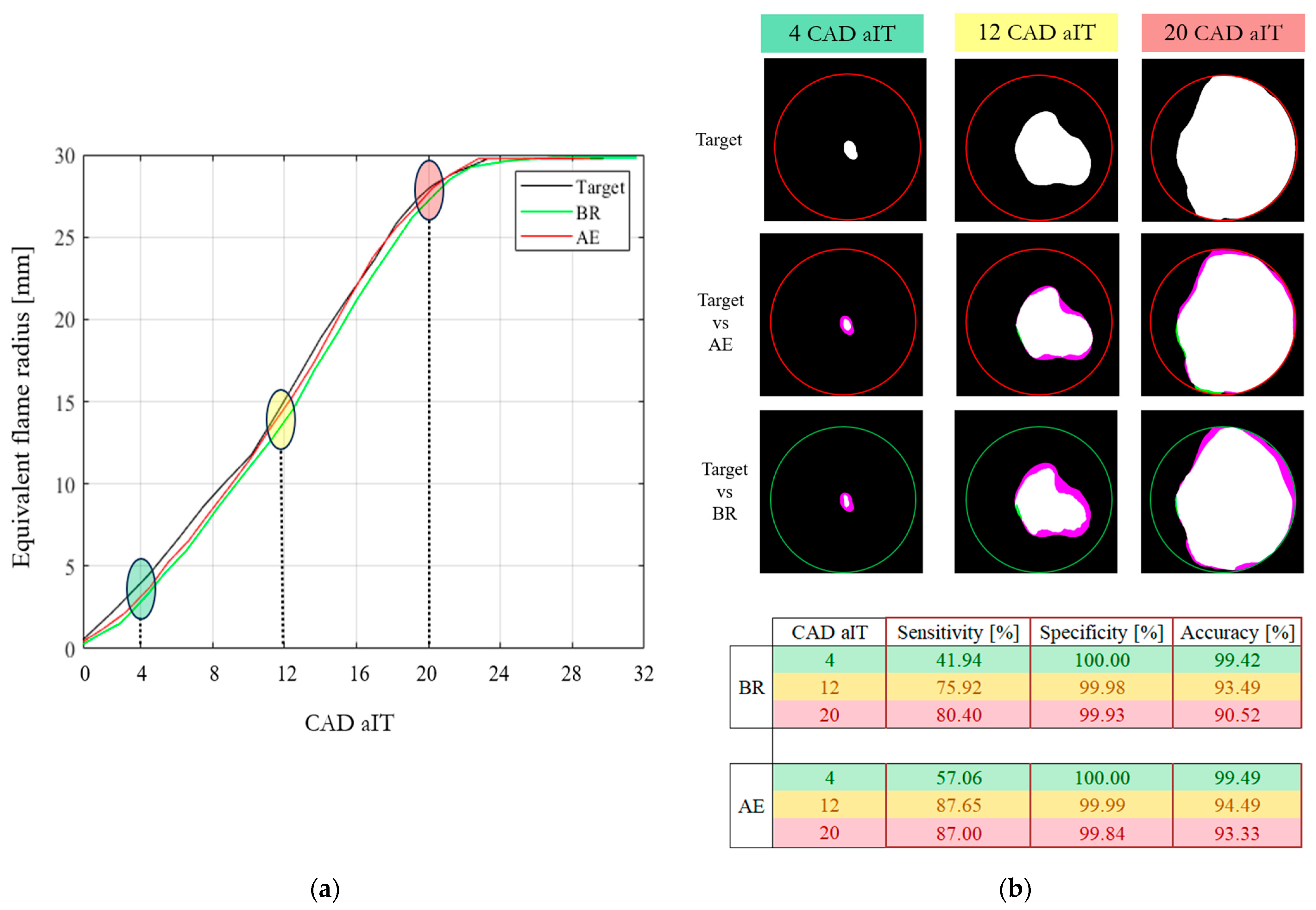
Figure 10a showcases the equivalent flame radius obtained from both methods, represented by the blue curve for BR and the red curve for AE. The target values, employed as a reference (depicted as the black line), will be used for comparison. No appreciable differences are found between the compared approaches.

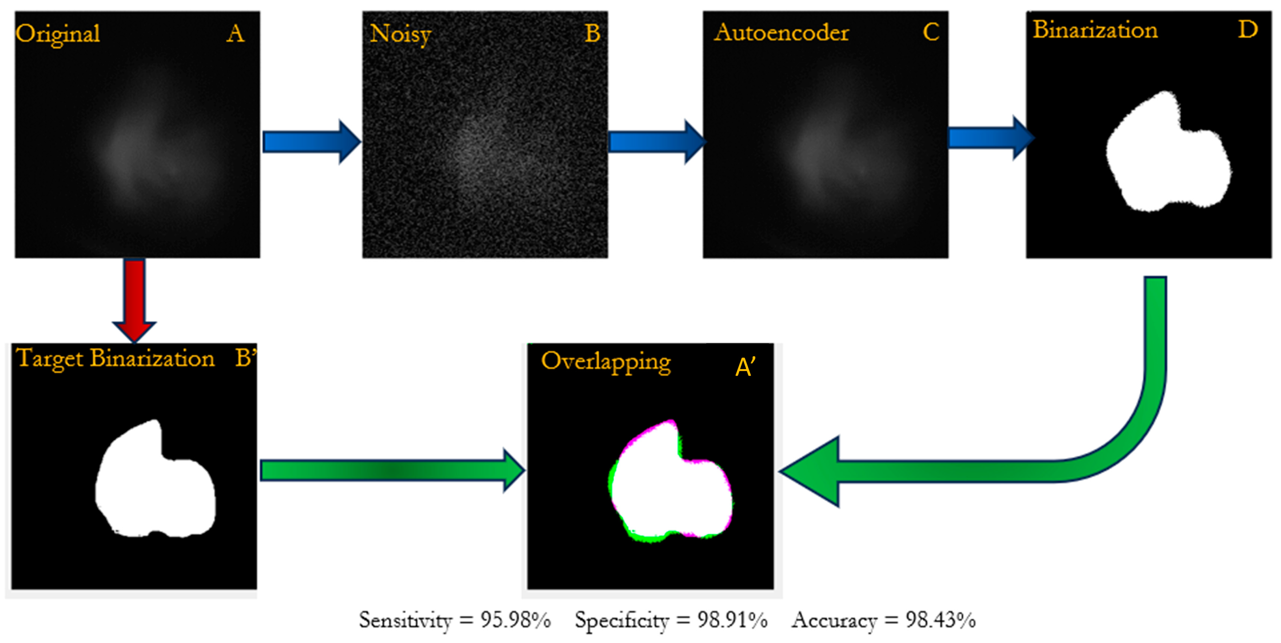
With slight underestimations in the first part of the combustion, i.e., kernel formation, both algorithms prove to be capable of effectively reproducing the target trend. A complementary analysis is carried out by overlapping the corresponding binarized images, as performed in Figure 9, at three representative frames after the ignition timing (IT), to quantify any over- and underestimations (Figure 10b).

This additional analysis is necessary to highlight how the proposed method, despite a slight underestimation of the front with respect to the target, still obtains a much better result than the BR method. Starting from the specificity levels, both algorithms show values equal to about 100%, testifying great proficiency in detecting pixels within the target boundary at each shown CAD aIT.

Concerning the sensitivity, the levels gradually increase as the flame front evolves, confirming the initial underestimation performed by both algorithms during the early stage of the combustion and their capability to progressively replicate the target as the process advances.

However, at 4 CAD aIT, there is a noticeable enhancement in AE’s capability to replicate the flame shape compared to BR. Specifically, the sensitivity level indicates an improvement of about 36% in performance by AE over BR (reaching approximately 57% for AE, compared to around 42% for BR).

Progressing further, an increase in BR enhances both sensitivity levels and AE, resulting in approximately a 16% increment at 12 CAD aIT and about an 8% increase at 20 CAD aIT.

The higher sensitivity levels of AE testify its superiority in accurately identifying pixels outside the flame edge as ‘no flame’, thereby indicating lower overestimations made by the proposed structure.

In terms of accuracy, AE exhibits improved performance compared to BR, showcasing a more comprehensive and precise delineation of the combustion evolution. Higher accuracy signifies a more comprehensive measure of the algorithm’s overall performance in correctly identifying both edge and non-edge pixels.

It accounts for true positives, true negatives, false positives, and false negatives, providing an inclusive evaluation of the algorithm’s precision in delineating the combustion evolution accurately.

Due to the impracticality in defining a target curve for all 63 recorded cycles, the outputs of both AE and BR are subsequently compared by considering data coming from the indicating analysis.

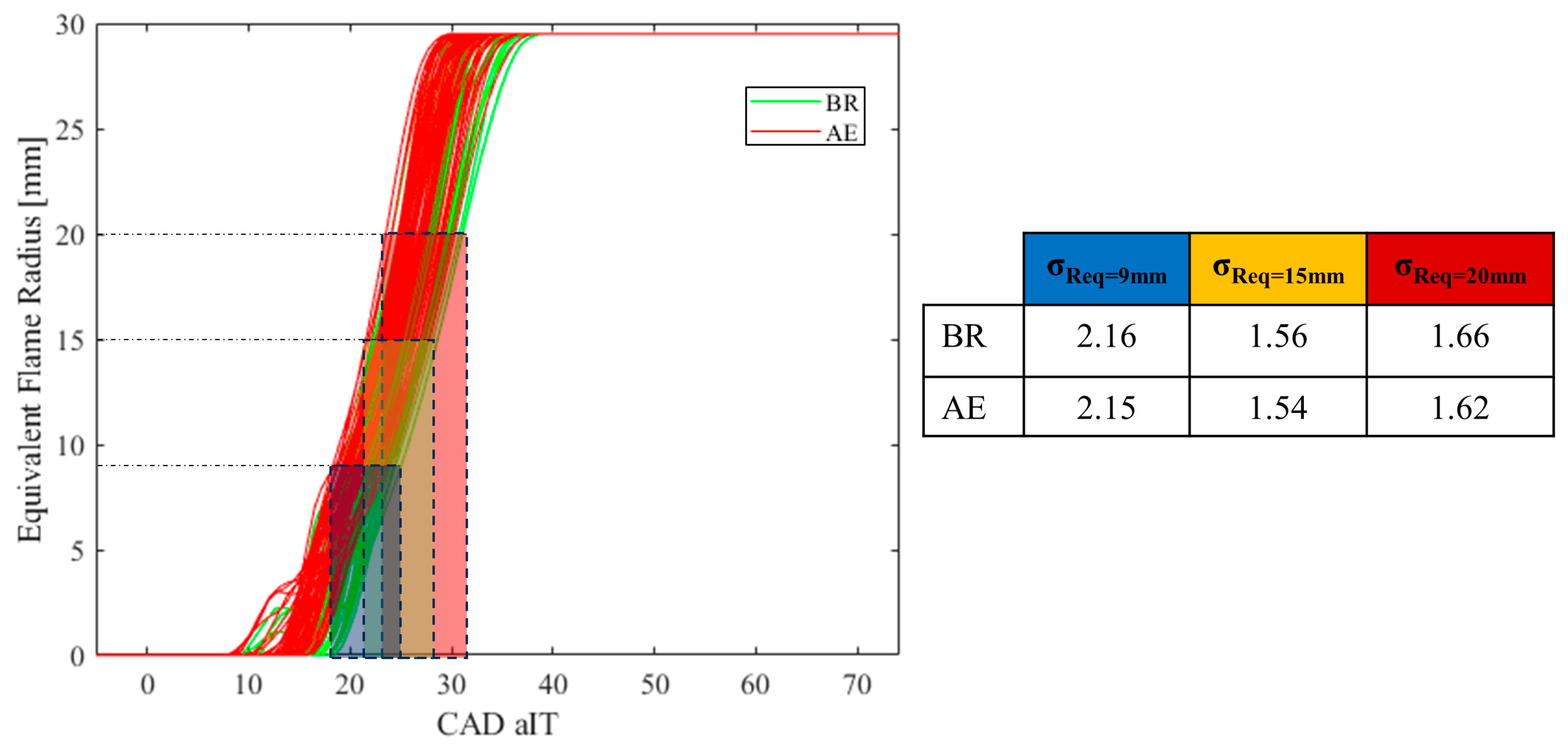
The curves depicted in Figure 11 represent the trend of the equivalent flame radius for all 63 combustion cases analyzed at λ = 1.0. The curves identified as BR and AE are narrow, indicating low dispersion. Low dispersion suggests high event repeatability, meaning minimal variation from cycle to cycle, consistent with the CoV_IMEP value recorded through the indicated analysis (Table 2). To quantify which of the two sets is narrower and therefore more faithful to the CoV_IMEP value, we consider the dispersion in CAD when the equivalent front radius is, for instance, equal to 9, 15, and 20 mm, i.e., σ_Req = 9 mm, σ_Req = 15 mm, σ_Req = 20 mm. This involves determining, for each R_eq calculated by both algorithms being compared, the CAD aIT corresponding to the first frame presenting, for example, R_eq ≥ 9, 15, and 20 mm. The uncertainty associated with identifying the CAD aIT where R_eq is equal to or exceeds 9, 15, or 20 mm reflects the variability inherent in the determination process. This variability aligns with the uncertainty observed in the data obtained from the KIBOX system analysis, and notably corresponds to the 0.6 CAD per frame sampling frequency of the high-speed camera. Looking at the three dispersion values displayed in Figure 11, during the initial flame front growth, both methods demonstrate similar dispersion levels. However, as the equivalent radius reaches 15 mm and 20 mm, AE shows superior performance compared to BR, displaying reduced dispersion values. This outcome could indicate a higher fidelity of AE with the experimental data if compared to BR.

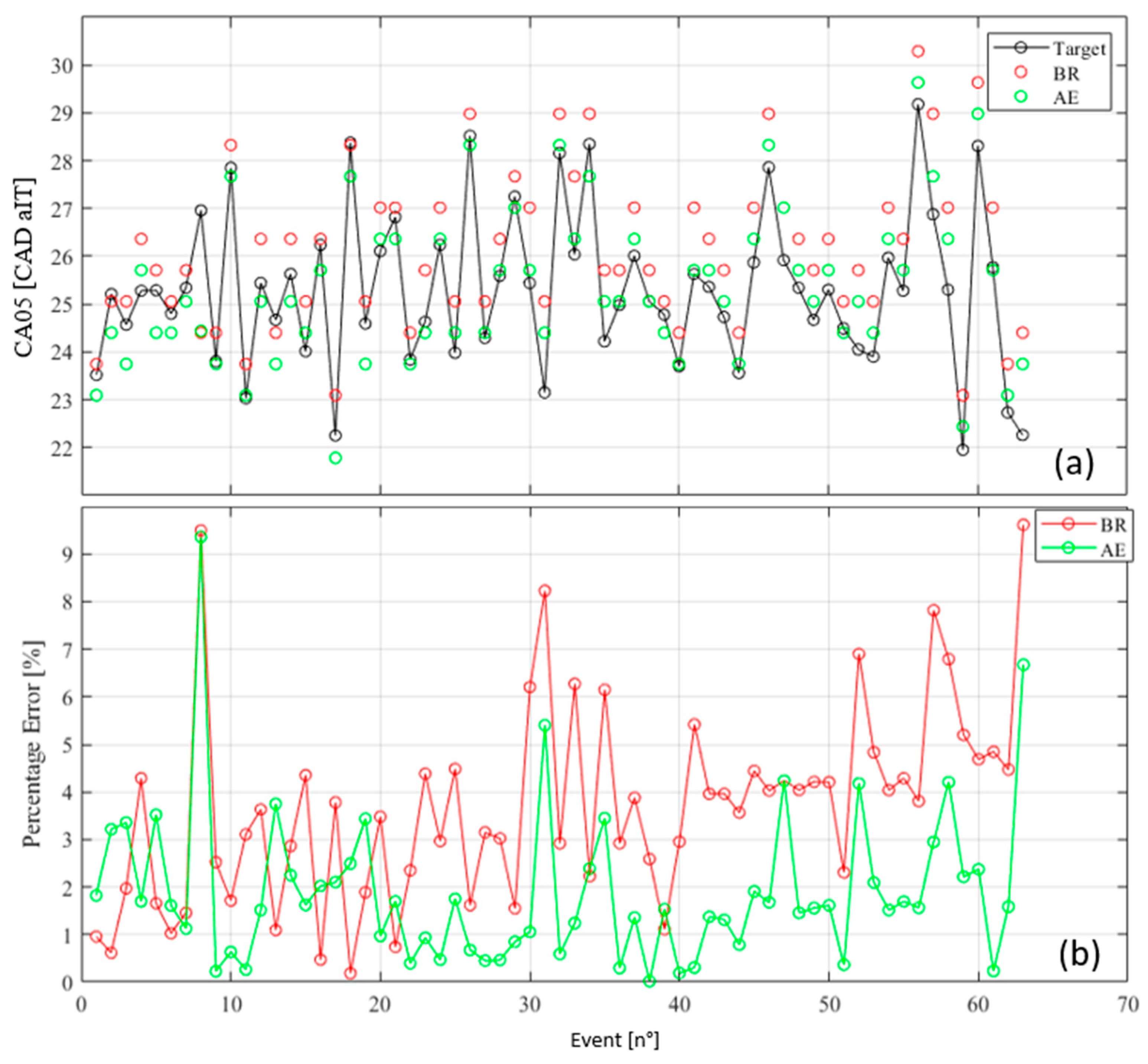
To better emphasize the latter outcome, another analysis can be performed by using the CA05 acquired from the indicating analysis. At λ = 1.0, the CA05 is derived from the equivalent flame radius value R_eq = 20 mm, as detailed in Section 2 [26]. Figure 12a presents the CA05 trend observed across the 63 cycles (depicted by black markers) alongside those estimated from the R_eq values generated by both algorithms (green markers for BR and red for AE). Meanwhile, Figure 12b illustrates the absolute difference (%Err = $\left|(\mathrm{C}\mathrm{A}\mathrm{D} \mathrm{a}\mathrm{I}\mathrm{T}-\mathrm{C}\mathrm{A}\mathrm{D} \mathrm{a}\mathrm{I}{\mathrm{T}}_{\mathrm{T}\mathrm{a}\mathrm{r}\mathrm{g}\mathrm{e}\mathrm{t}})/\mathrm{C}\mathrm{A}\mathrm{D} \mathrm{a}\mathrm{I}{\mathrm{T}}_{\mathrm{T}\mathrm{a}\mathrm{r}\mathrm{g}\mathrm{e}\mathrm{t}}\right|\times 100$) between the estimation of CAD aIT corresponding to the appearance of CA05 performed by the compared algorithm and the target. In this analysis, the CAD aIT of CA05 identified by the indicating system is referred to as the target value.

As observable from the graph, AE demonstrates lesser deviation from the target compared to BR. Specifically, except for a few sporadic instances, the proposed algorithm maintains the difference below 4% in 57 out of 63 cases, equal to 90%. In contrast, BR exhibits a discrepancy exceeding 4% in 40% of the cases. Therefore, this outcome signifies a better alignment of the data from the indicated analysis, indicating a greater confidence of the AE algorithm in physically reproducing the front development.

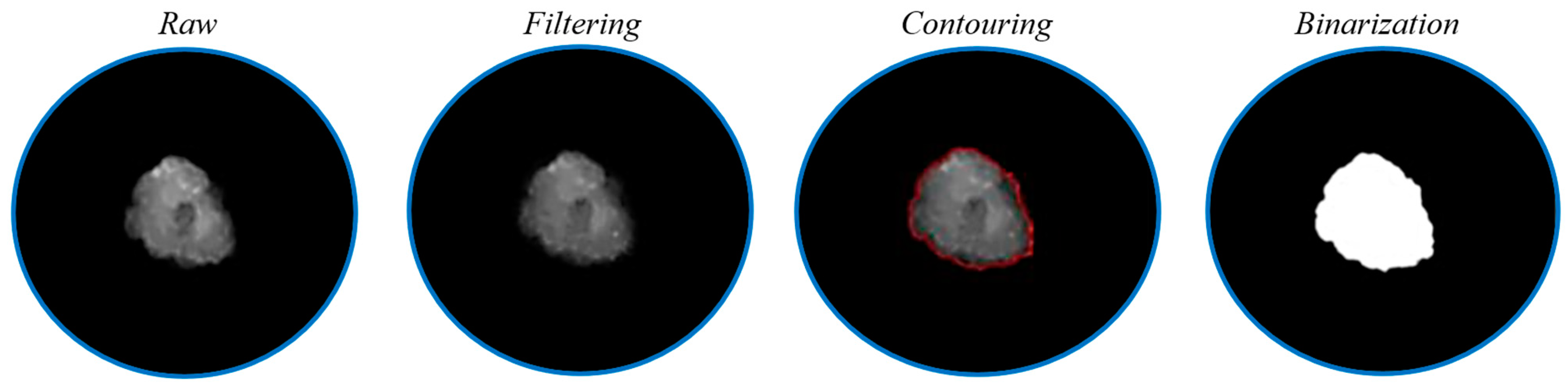
The binarization process following the autoencoder outperforms alternative post-processing methods in flame front evolution detection due to its ability to exploit the learned representations within the autoencoder’s latent space. This process effectively translates the extracted features into a clearer and more distinct delineation of the flame front, resulting in enhanced precision and accuracy compared to other algorithms that might not leverage such learned representations.

Consequently, this approach does not require specific threshold exploration, which can be laborious. For instance, unlike the BR case that necessitates semi-automatic threshold searches, the AE case employs a standard binarization algorithm.

This independence from user intervention results in reduced workload, as the AE process is entirely automated. Further, as evident from the results, this method exhibits greater reliability in its output.

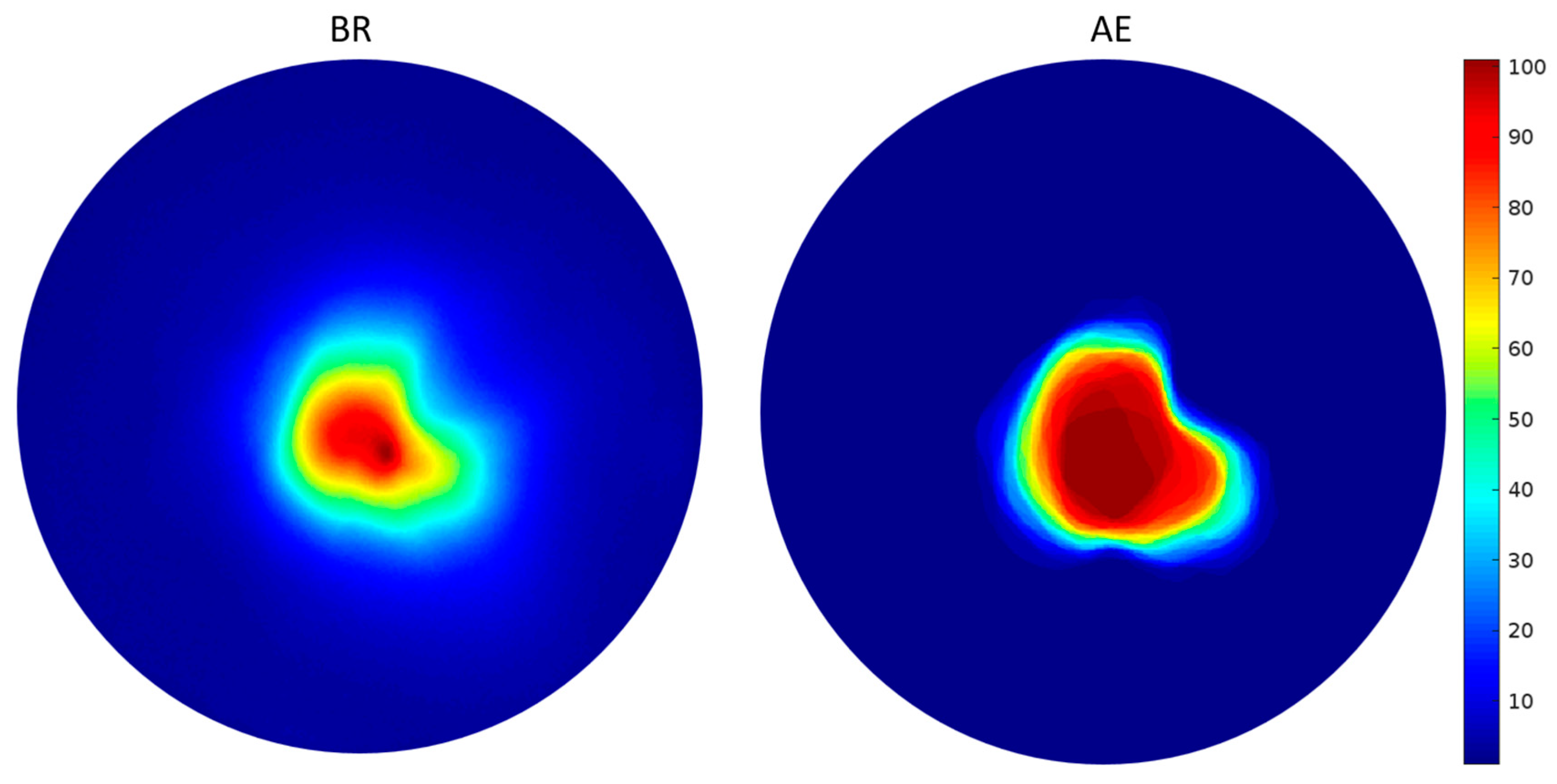
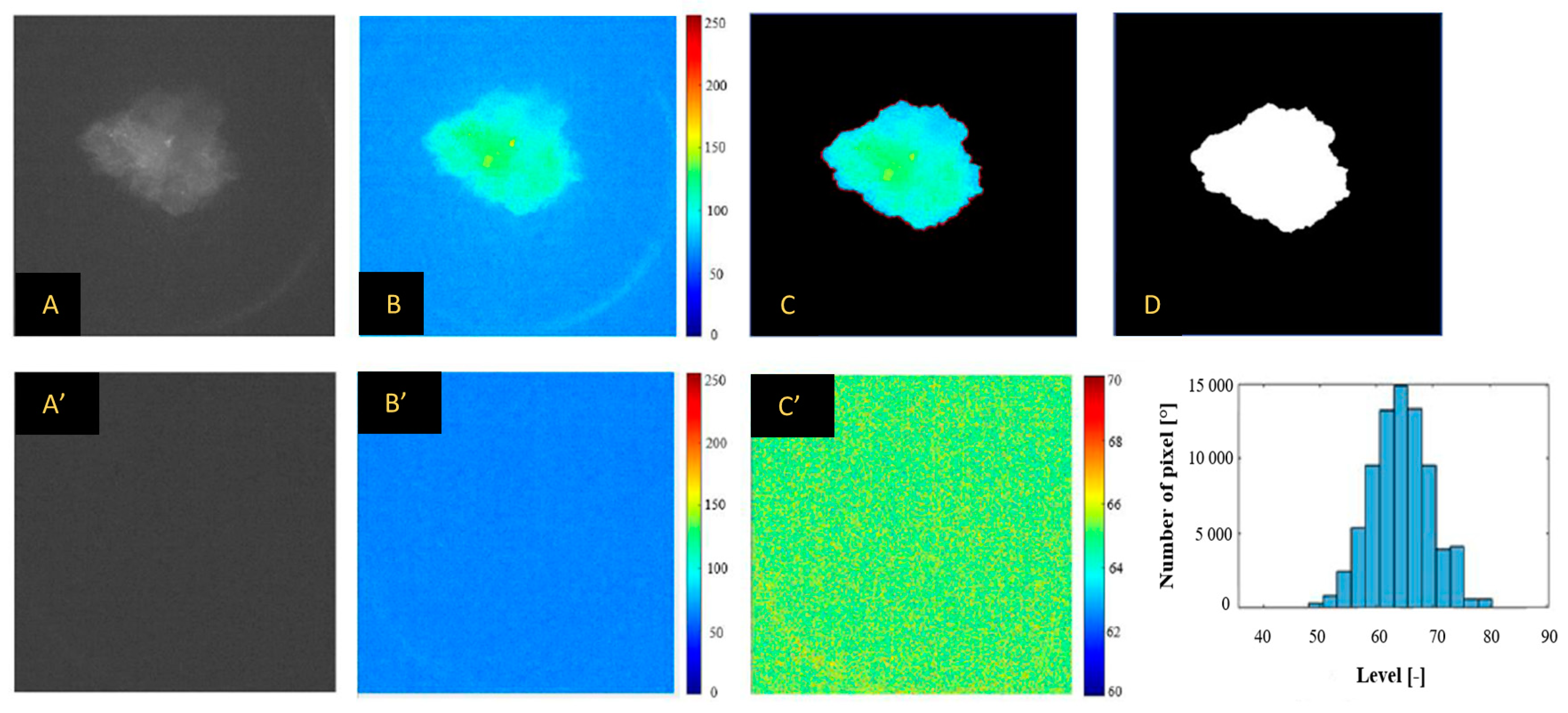
To better emphasize the obtained outcomes, Figure 13 reports the early flame spatial repeatability when Req = 9 mm. The image is obtained by averaging the luminosity levels of the 63 consecutive values, i.e., by means of the flame probability presence when the mean equivalent flame radius is equal to 9 mm [21]. The autoencoder effectively eliminates noise, evidenced by the near absence of gradients beyond the flame front boundary and reduced internal gradients. This precision is notable in the high-probability flame zone, which is distinctly clearer if compared to the BR approach. This underscores two crucial points, i.e., AE aligns with the evaluation of CoV_IMEP from the indicated analysis, where a larger flame area corresponds to greater stability, consistent with the λ = 1.0 scenario, and, moreover, it demonstrates a stronger ability to detect the initial flame development if compared to the BR method. In summary, the autoencoder achieves superior precision in flame front segmentation, aligning with the indicated analysis’s stability assessment and outperforming the BR method in early flame evolution detection.

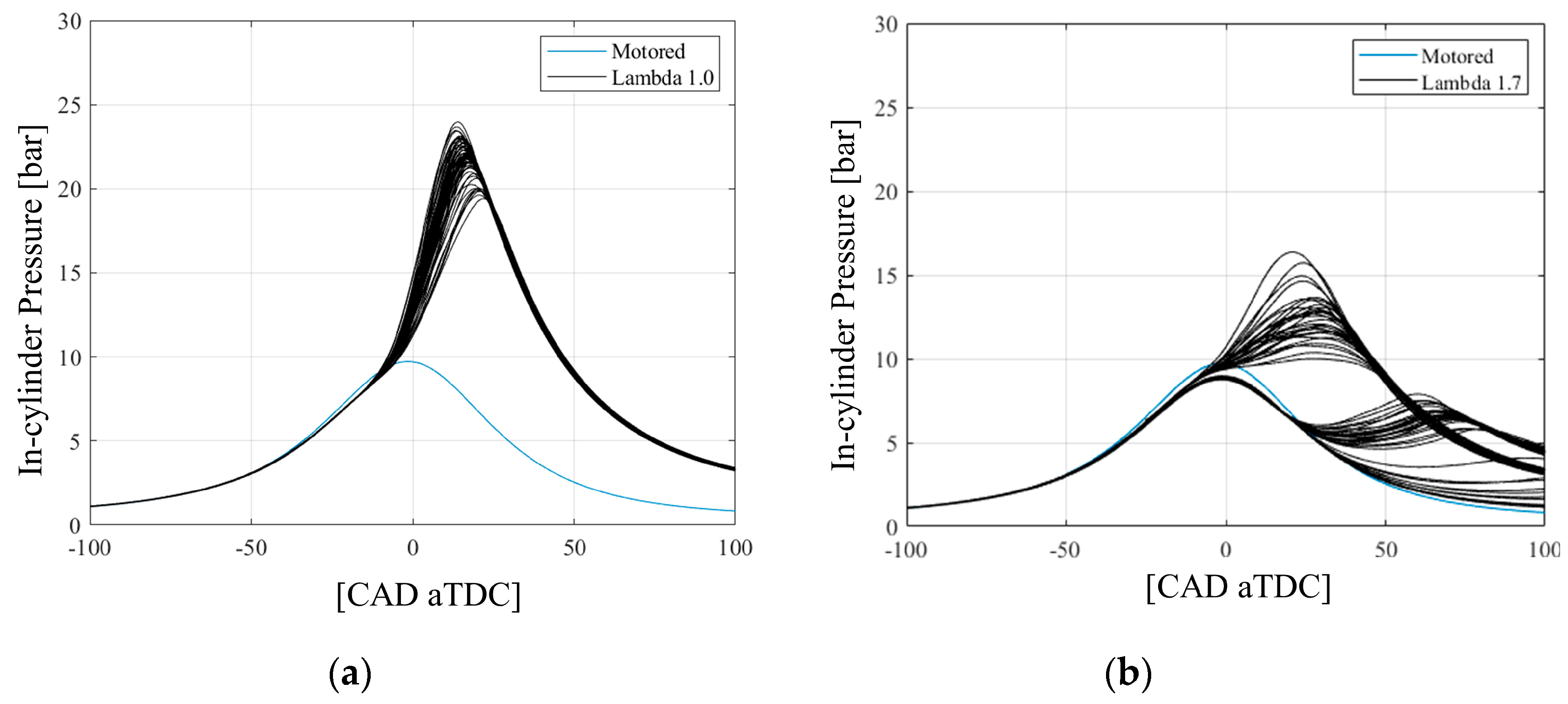
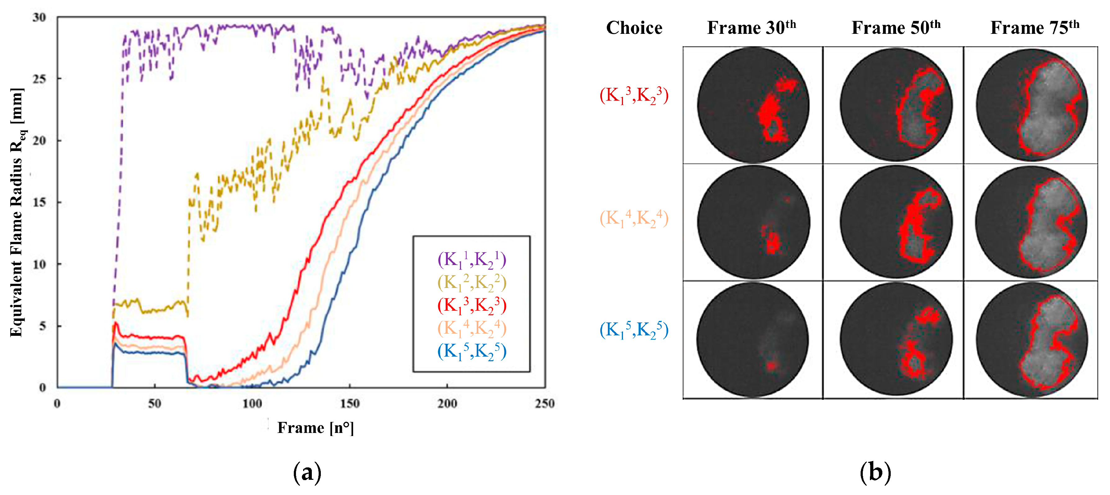
By examining Figure 2b, three distinct behaviors can be identified summarily. The first relates to the curve exhibiting the highest-pressure level, the second is associated with combustion featuring delayed ignitions, and the third set of curves highlights abnormal combustion occurrences such as misfires. Following an evaluation of the proposed ANN structure in this study at a specific setting (λ = 1.0), a combustion event was selected for each of the abovementioned groups to gauge the autoencoder’s performance against BR under critical conditions (λ = 1.7). 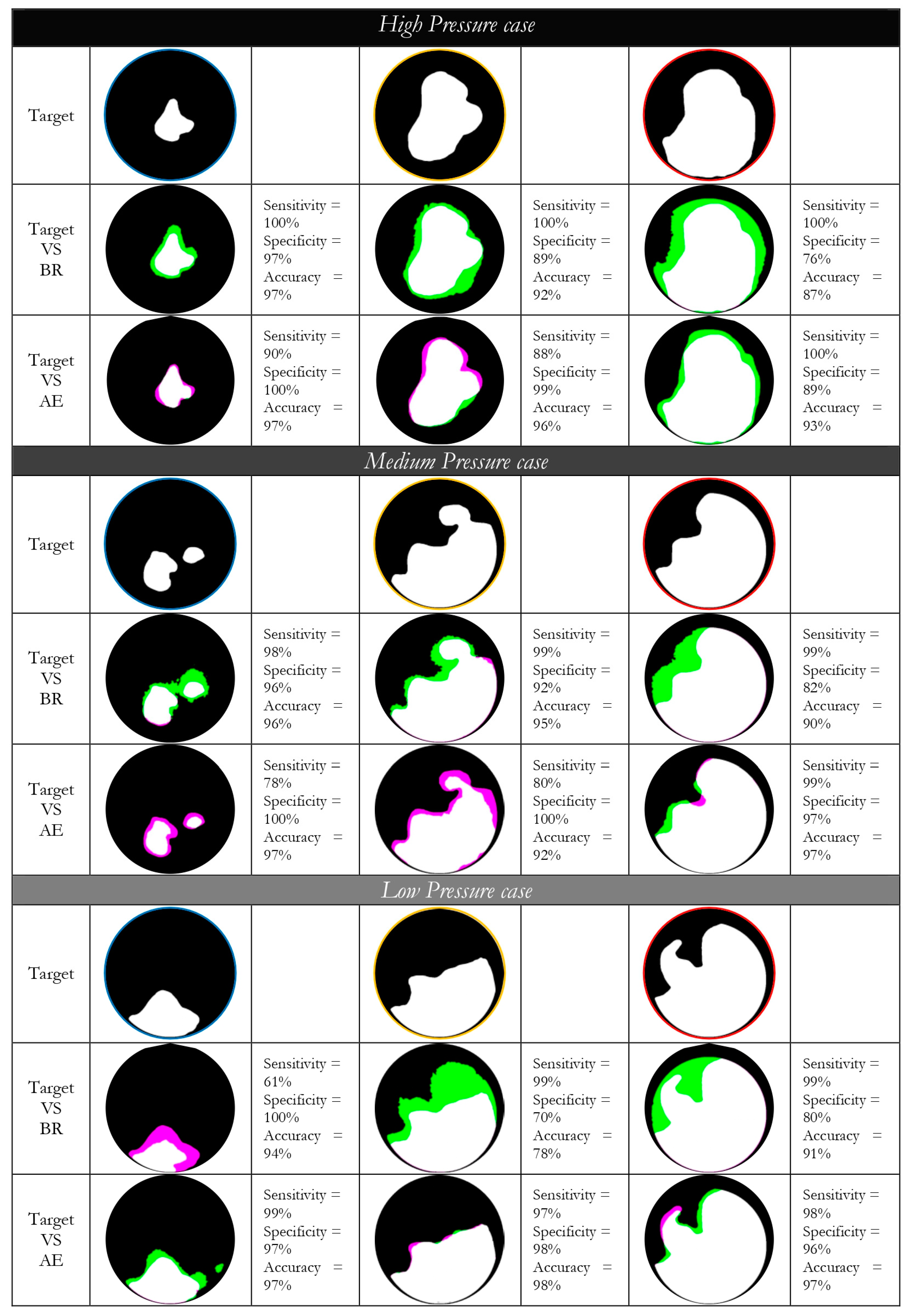As previously demonstrated at λ = 1.0 in Figure 1, similar assessments have been conducted, and the corresponding outcomes are presented in Figure 14.

Starting with the ‘High Pressure’ combustion events, in Frame 1, both methods exhibit promising results. BR achieves a perfect sensitivity of 100%, indicating its ability to correctly identify all positive cases. However, its specificity is at 97%, suggesting the possibility of some false positives. The overall accuracy stands at 97%. On the other hand, AE maintains a sensitivity of 90%, with no false positives (specificity of 100%). Despite sacrificing a small part of sensitivity, it achieves a higher specificity, and accuracy remains at 97%. Moving to Frame 2, BR sustains a high sensitivity of 100%, but its specificity decreases to 89%, implying a higher likelihood of false positives. The accuracy in this frame is 92%. AE exhibits a sensitivity of 88%, a slight reduction compared to BR. However, its specificity significantly improves to 99%, indicating greater precision in negative cases. The accuracy is 96%. In Frame 3, BR maintains a sensitivity of 100%, but both specificity and accuracy decrease to 76% and 87%, respectively. AE sustains a sensitivity of 100%, and its specificity is at 89%, with an accuracy of 93%. Once again, AE maintains higher specificity compared to BR.

Moving on to the scenario of ‘Medium Pressure’, in Frame 1, BR demonstrates a sensitivity of 98%, meaning it can accurately identify 98% of positive cases. The specificity is at 96%, suggesting a relatively low rate of false positives, and the overall accuracy is 96%. In comparison, AE exhibits a sensitivity of 78%, indicating a lower ability to correctly identify positive cases. However, it compensates with a perfect specificity of 100%, resulting in an accuracy of 97%. Moving to Frame 2, BR achieves a sensitivity of 99% with a specificity of 92% and an accuracy of 95%. The high sensitivity suggests the effective identification of positive cases, but the lower specificity implies a higher likelihood of false positives. AE, on the other hand, maintains a sensitivity of 80% and a perfect specificity of 100%, resulting in an accuracy of 92%. In Frame 3, BR maintains a high sensitivity of 99%, but both specificity and accuracy decrease to 82% and 90%, respectively. In contrast, AE sustains a sensitivity of 99% with a specificity of 97%, leading to an accuracy of 97%.

Lastly, addressing the circumstances involving ‘Low Pressure’, in Frame 1, BR displays a sensitivity of 61%, indicating its ability to correctly identify 61% of positive cases. The specificity is at 100%, implying an absence of false positives, and the overall accuracy is 94%. On the other hand, AE achieves a higher sensitivity of 99%, coupled with a specificity of 97%, resulting in an accuracy of 97%. In Frame 2, BR attains a sensitivity of 99%, suggesting the effective identification of positive cases. However, the specificity is lower at 70%, leading to a higher likelihood of false positives, and the accuracy is 78%. AE, in contrast, maintains a sensitivity of 97% and a higher specificity of 98%, resulting in an accuracy of 98%. Moving to Frame 3, BR maintains a high sensitivity of 99%, but both specificity and accuracy decrease to 80% and 91%, respectively. AE sustains a sensitivity of 98%, a specificity of 96%, and an accuracy of 97%. The comparisons between the equivalent flame radius confirm the superiority of AE in comparison to BR in reproducing the Req target.

In summary, AE tends to demonstrate a more balanced and consistent performance across various scenarios, especially excelling in specificity and precision. BR, while achieving high sensitivity, may encounter challenges in maintaining specificity, impacting its ability to avoid false positives. Considering these outcomes, it is correct to conclude that there is a noticeable decrease in BR’s performance and an increase in AE’s performance across the frames. This gradual difference in performance suggests that AE is more suitable for lean combustions, showing increased and consistent performance, especially in anomalous combustion scenarios, making it superior to BR. In summary, the observations align with the idea that AE is better suited for the scenarios presented, offering improved performance over BR, especially in terms of specificity and the ability to handle ultra-lean and anomalous combustions.

4. Conclusions

The present study presents a comprehensive analysis and comparison between the base reference method (BR) and the proposed autoencoder (AE) for flame front evolution detection in combustion processes.

4.1. Obtained Findings

Through a meticulous evaluation and comparative analysis, it is evident that AE, leveraging its autoencoder architecture, surpasses BR in several aspects.

The evaluation metrics employed for performance assessment, including sensitivity, specificity, and accuracy, affirm the superior performance of AE over BR. Notably, AE demonstrates higher sensitivity levels, indicating its superior capability in accurately identifying pixels outside the flame edge, resulting in lower overestimations. Additionally, AE showcases improved accuracy, accurately delineating both edge and non-edge pixels, which is vital in accurately representing the combustion evolution.

The AE’s robustness and reliability are further accentuated by its independence from specific threshold exploration, which is a notable requirement in the BR methodology. By employing a standard binarization algorithm and leveraging learned representations within its latent space, AE achieves enhanced precision and accuracy in delineating the flame front evolution without laborious threshold searches.

Furthermore, the comparison with the manually obtained binarized image and the target, as well as the analysis of early flame development, consistently highlights AE’s ability to align with CoV_IMEP from the indicated analysis and its superior performance in early flame evolution detection compared to the BR method.

Overall, the results underscore the efficacy of AE in accurately reproducing and delineating the combustion evolution compared to the established BR method. AE’s advanced capabilities, automated processing, and superior performance metrics position it as a promising methodology for accurate flame front evolution detection in combustion processes. Building on this observation, the comprehensive study underscores AE’s superiority over BR in flame front evolution detection in combustion processes. The evaluation metrics, including sensitivity, specificity, and accuracy, consistently highlight AE’s enhanced performance. AE’s ability to achieve higher sensitivity and improved accuracy, along with its independence from specific threshold exploration, positions it as a promising methodology for accurate flame front evolution detection in combustion processes. The results emphasize AE’s advanced capabilities, automated processing, and superior performance metrics, affirming its potential as a reliable and effective alternative to the established BR method especially when operating with ultra-lean or anomalous combustion events.

4.2. Potential Challenges and Limitations of the Autoencoder Approach

One primary challenge is connected to the computational efficiency and scalability of the proposed approach. While the presented outcomes showed promising results, the applicability of the autoencoder approach for large-scale industrial engines may be limited. In fact, in the present work, the proposed architecture was trained on an image of one operational scenario and applied to all other cases. However, in real-engine applications, when dealing with different engines and varied operating conditions, the method still requires training on a high amount of data for generalizability, leading to increased time and resource expenditure.

4.3. Future Works

Considering the abovementioned challenges, future research will be focused on addressing practical limitations with the aim of enhancing both applicability and robustness of the autoencoder approach in real-engine testing and industrial applications. The target is to evaluate the integration of an autoencoder into industrial practices, thereby unlocking its full potential in optimizing engine performance and emissions control. Future works will therefore be focused on applying the proposed method at various operating conditions, by varying, for instance, the engine speed, lambda condition, type of fuel, and load condition to generalize the proposed approach.

References

1. Wijeyakulasuriya, S.; Kim, J.; Probst, D.; Srivastava, K.; Yang, P.; Scarcelli, R.; Senecal, P.K. Enabling powertrain technologies for Euro 7/VII vehicles with computational fluid dynamics. Transp. Eng. 2022, 9, 100127. [Google Scholar] [CrossRef]
2. Petrucci, L.; Ricci, F.; Mariani, F.; Mariani, A. From real to virtual sensors, an artificial intelligence approach for the industrial phase of end-of-line quality control of GDI pumps. Measurement 2022, 199, 111583. [Google Scholar] [CrossRef]
3. Petrucci, L.; Ricci, F.; Mariani, F.; Cruccolini, V.; Violi, M. Engine Knock Evaluation Using a Machine Learning Approach (No. 2020-24-0005); SAE International: Warrendale, PA, USA, 2020. [Google Scholar]
4. Chen, L.; Wei, H.; Zhang, R.; Pan, J.; Zhou, L.; Feng, D. Effects of spark plug type and ignition energy on combustion performance in an optical SI engine fueled with methane. Appl. Therm. Eng. 2019, 148, 188–195. [Google Scholar] [CrossRef]
5. Uddeen, K.; Tang, Q.; Shi, H.; Magnotti, G.; Turner, J. A novel multiple spark ignition strategy to achieve pure ammonia combustion in an optical spark-ignition engine. Fuel 2023, 349, 128741. [Google Scholar] [CrossRef]
6. Dahham, R.Y.; Wei, H.; Pan, J. Improving thermal efficiency of internal combustion engines: Recent progress and remaining challenges. Energies 2022, 15, 6222. [Google Scholar] [CrossRef]
7. Zembi, J.; Ricci, F.; Grimaldi, C.; Battistoni, M. Numerical Simulation of the Early Flame Development Produced by a Barrier Discharge Igniter in an Optical Access Engine (No. 2021-24-0011); SAE Technical Paper; SAE International: Warrendale, PA, USA, 2021. [Google Scholar]
8. Lu, Y.; Morris, S.; Kook, S. Effects of injection pressure on the flame front growth in an optical direct injection spark ignition engine. Appl. Therm. Eng. 2022, 214, 118848. [Google Scholar] [CrossRef]
9. Aliramezani, M.; Koch, C.R.; Shahbakhti, M. Modeling, diagnostics, optimization, and control of internal combustion engines via modern machine learning techniques: A review and future directions. Prog. Energy Combust. Sci. 2022, 88, 100967. [Google Scholar] [CrossRef]
10. Russo, A.; Lax, G. Using artificial intelligence for space challenges: A survey. Appl. Sci. 2022, 12, 5106. [Google Scholar] [CrossRef]
11. Ineza Havugimana, L.F.; Liu, B.; Liu, F.; Zhang, J.; Li, B.; Wan, P. Review of Artificial Intelligent Algorithms for Engine Performance, Control, and Diagnosis. Energies 2023, 16, 1206. [Google Scholar] [CrossRef]
12. Olugbade, S.; Ojo, S.; Imoize, A.L.; Isabona, J.; Alaba, M.O. A review of artificial intelligence and machine learning for incident detectors in road transport systems. Math. Comput. Appl. 2022, 27, 77. [Google Scholar] [CrossRef]
13. Rani, S.; Ghai, D.; Kumar, S. Object detection and recognition using contour based edge detection and fast R-CNN. Multimed. Tools Appl. 2022, 81, 42183–42207. [Google Scholar] [CrossRef]
14. Li, Y.; Chai, G.; Wang, Y.; Lei, L.; Zhang, X. Ace r-cnn: An attention complementary and edge detection-based instance segmentation algorithm for individual tree species identification using uav rgb images and lidar data. Remote Sens. 2022, 14, 3035. [Google Scholar] [CrossRef]
15. Petrucci, L.; Ricci, F.; Martinelli, R.; Mariani, F. Detecting the Flame Front Evolution in Spark-Ignition Engine under Lean Condition Using the Mask R-CNN Approach. Vehicles 2022, 4, 978–995. [Google Scholar] [CrossRef]
16. Shawal, S.; Goschutz, M.; Schild, M.; Kaiser, S.; Neurohr, M.; Pfeil, J.; Koch, T. High-speed imaging of early flame growth in spark-ignited engines using different imaging systems via endoscopic and full optical access. SAE Int. J. Engines 2016, 9, 704–718. [Google Scholar] [CrossRef]
17. Heydarian, M.; Doyle, T.E.; Samavi, R. MLCM: Multi-label confusion matrix. IEEE Access 2022, 10, 19083–19095. [Google Scholar] [CrossRef]
18. Zheng, Q.; Zheng, L.; Deng, J.; Li, Y.; Shang, C.; Shen, Q. Transformer-based hierarchical dynamic decoders for salient object detection. Knowl.-Based Syst. 2023, 282, 111075. [Google Scholar] [CrossRef]
19. Xing, Y.; Zhong, L.; Zhong, X. An encoder-decoder network based FCN architecture for semantic segmentation. Wirel. Commun. Mob. Comput. 2020, 2020, 8861886. [Google Scholar] [CrossRef]
20. Stahlberg, F. Neural machine translation: A review. J. Artif. Intell. Res. 2020, 69, 343–418. [Google Scholar] [CrossRef]
21. Bank, D.; Koenigstein, N.; Giryes, R. Autoencoders. In Machine Learning for Data Science Handbook: Data Mining and Knowledge Discovery Handbook; Springer: Berlin/Heidelberg, Germany, 2023; pp. 353–374. [Google Scholar]
22. Karimpouli, S.; Tahmasebi, P. Segmentation of digital rock images using deep convolutional autoencoder networks. Comput. Geosci. 2019, 126, 142–150. [Google Scholar] [CrossRef]
23. Cheng, Z.; Sun, H.; Takeuchi, M.; Katto, J. Deep convolutional autoencoder-based lossy image compression. In Proceedings of the 2018 Picture Coding Symposium (PCS), San Francisco, CA, USA, 24–27 June 2018; pp. 253–257. [Google Scholar]
24. Posch, S.; Gößnitzer, C.; Ofner, A.B.; Pirker, G.; Wimmer, A. Modeling cycle-to-cycle variations of a spark-ignited gas engine using artificial flow fields generated by a variational autoencoder. Energies 2022, 157, 2325. [Google Scholar] [CrossRef]
25. Heywood, J.B. Internal Combustion Engine Fundamentals; McGraw-Hill: New York, NY, USA, 1988. [Google Scholar]
26. Martinelli, R.; Ricci, F.; Zembi, J.; Battistoni, M.; Grimaldi, C.; Papi, S. Lean Combustion Analysis of a Plasma-Assisted Ignition System in a Single Cylinder Engine Fueled with E85 (No. 2022-24-0034); SAE Technical Paper; SAE International: Warrendale, PA, USA, 2022. [Google Scholar]
27. Islam, M.Z.; Islam, M.M.; Asraf, A. A combined deep CNN-LSTM network for the detection of novel coronavirus (COVID-19) using X-ray images. Inform. Med. Unlocked 2020, 20, 100412. [Google Scholar] [CrossRef] [PubMed]
28. Vincent, P.; Larochelle, H.; Bengio, Y.; Manzagol, P.-A. Extracting and composing robust features with denoising autoencoders. In Proceedings of the 25th International Conference on Machine Learning, Helsinki, Finland, 5–9 July 2008; ACM: New York, NY, USA, 2008; pp. 1096–1103. [Google Scholar]
29. Choi, H.; Kim, M.; Lee, G.; Kim, W. Unsupervised learning approach for network intrusion detection system using autoencoders. J. Supercomput. 2019, 75, 5597–5621. [Google Scholar] [CrossRef]
30. Shen, Q.; Wang, G.; Wang, Y.; Zeng, B.; Yu, X.; He, S. Prediction Model for Transient NOx Emission of Diesel Engine Based on CNN-LSTM Network. Energies 2023, 16, 5347. [Google Scholar] [CrossRef]
31. SAE J1832 Low Pressure Gasoline Fuel Injector; SAE International: Warrendale, PA, USA, 2001.
Figure 1. (a) Single-cylinder research engine and (b) schematic representation of optical access.
Energies 17 01759 g001
Figure 2. Comparison between the in-cylinder pressures for each operating condition (black lines), at (a) λ = 1.0 and (b) λ = 1.7 against the motored case (blue line) averaged over the 63 recorded cycles.
Energies 17 01759 g002
Figure 3. Variation in flame front brightness with λ: the images illustrate flame front changes across different λ conditions. Increasing λ values showcase consistent flame sizes alongside decreasing brightness. Additionally, critical condition images highlight reduced luminosity and quartz fouling due to incomplete combustion phenomena.
Energies 17 01759 g003
Figure 4. Representation of the main post-processing steps applied to the original image.
Energies 17 01759 g004
Figure 5. (a) Some instances of Req that fail to accurately depict the flame radius’s progressive growth during combustion development, contrasted with Req (solid lines) that appear promising for replicating this physical phenomenon in combustion. (b) On the right-hand side, an illustration of the contouring process applied to the potentially suitable cases, assessing the base reference algorithm’s ability to reproduce the original images’ flame fronts. The selection of (K13, K23) enhances flame front reproduction, suggesting it as the optimal choice.
Energies 17 01759 g005
Figure 6. Simplified representation of a stacked denoising autoencoder.
Energies 17 01759 g006
Figure 7. (A) The main steps to create the target image for comparison with the proposed algorithm’s output involve several key processes. (B) The definition of the noise level to be subtracted from image (B) in order to derive image (C) is crucial. Image (A′) represents an image with no flame occurring, utilized as a reference to establish the noise level. Meanwhile, figure (B′) visually represents image (A′) in false colors. On the other hand, (C′) highlights the average level of (A′) across the entire spectrum, ranging from the minimum to the maximum level. The histogram presented on the right-hand side illustrates the distribution of pixel levels in (C′). Lastly, image (D) showcases the outcome of the binarization process, presumably after the aforementioned steps have been executed. This final image serves as a product of the preceding processes, presumably depicting the desired target for comparison with the output generated by the proposed algorithm. The histogram on the right side shows the level distribution of the pixels of (C′).
Energies 17 01759 g007
Figure 8. Architecture of the optimized proposed autoencoder.
Energies 17 01759 g008
Figure 9. Output of the autoencoder in the preliminary analysis aimed to assess the performance of the proposed architecture and comparison with the binarized image of the flame front manually obtained and used as the target. A is the original image while the other ones are the images post-processed according to the procedures reported in the Section 2.3.2.
Energies 17 01759 g009
Figure 10. (a) Comparison among the target equivalent radius (black line), obtained through the manual binarization of images as explained in Section 4.1; the one obtained through BR as per Section 4.1 (green line); and that obtained from AE, according to Section 4.2 (red line). (b) Comparison among the binarized images using the three aforementioned methodologies conducted at three different CAD values indicated in (a) by green (4 CAD aIT), yellow (12 CAD aIT), and red (20 CAD aIT) circles with their respective confusion matrix values.
Energies 17 01759 g010
Figure 11. Variation of equivalent flame radius for 63 combustion cases at λ = 1.0. Narrow BR and AE curves indicate low dispersion, suggesting high repeatability. Dispersion is compared in CAD at 9 (blue), 15 (yellow), and 20 (red) mm of the equivalent front radius to determine fidelity to the indicating analysis.
Energies 17 01759 g011
Figure 12. (a) displays the trend of CA05 observed across 63 cycles (represented by black markers) compared to estimations derived from Req values by both algorithms (BR in red and AE in green). (b) showcases the absolute relative difference %Err between the CAD aIT estimations for the appearance of MFB50 by the compared algorithm and the target.
Energies 17 01759 g012
Figure 13. The probability of the presence of an early flame for Req = 9 mm. The red area indicates 100% of probability of finding the discharge or the flame while the blue one indicates 0% probability.
Energies 17 01759 g013
Figure 14. Comparative performance analysis of the burner recognition (BR) and autoencoder (AE) in various combustion scenarios at λ = 1.7. Each column represents three distinct instances of flame development, which depict the beginning, middle, and end of the combustion event. In low-pressure cases, flame development progresses slower compared to high-pressure cases. Therefore, the same column does not refer to the same CAD but rather to the same stage of combustion evolution. BR exhibits high sensitivity but varying specificity across frames, while AE demonstrates consistent and balanced performance, excelling in specificity and precision. The results suggest AE’s superiority, particularly in lean and anomalous combustion scenarios.
Energies 17 01759 g014