Breathing Planet Earth: Analysis of Keeling’s Data on CO₂ and O₂ with Respiratory Quotient (RQ), Part II: Energy-Based Global RQ and CO₂ Budget

Abstract

For breathing humans, the respiratory quotient (RQ = CO₂ moles released/O₂ mols consumed) ranges from 0.7 to 1.0. In Part I, the literature on the RQ was reviewed and Keeling’s data on atmospheric CO₂ and O₂ concentrations (1991–2018) were used in the estimation of the global RQ as 0.47. A new interpretation of RQ_Glob is provided in Part II by treating the planet as a “Hypothetical Biological system (HBS)”. The CO₂ and O₂ balance equations are adopted for estimating (i) energy-based RQ_Glob(En) and (ii) the CO₂ distribution in GT/year and % of CO₂ captured by the atmosphere, land, and ocean. The key findings are as follows: (i) The RQ_Glob(En) is estimated as 0.35 and is relatively constant from 1991 to 2020. The use of RQ_Glob(En) enables the estimation of CO₂ added to the atmosphere from the knowledge of annual fossil fuel (FF) energy data; (ii) The RQ method for the CO₂ budget is validated by comparing the annual CO₂ distribution results with results from more detailed models; (iii) Explicit relations are presented for CO₂ sink in the atmosphere, land, and ocean biomasses, and storage in ocean water from the knowledge of curve fit constants of Keeling’s curves and the RQ of FF and biomasses; (iv) The rate of global average temperature rise (0.27 °C/decade) is predicted using RQ_Glob,(En) and the annual energy release rate and compared with the literature data; and (v) Earth’s mass loss in GT and O₂ in the atmosphere are predicted by extrapolating the curve fit to the year 3700. The effect of RQ_Glob and RQ_FF on the econometry and policy issues is briefly discussed.

1. Introduction

Atmospheric oxygen production on Earth started about 3.2 billion years ago. The total O₂ produced was estimated at 5.63 × 10⁵ Peta moles with 0.375 × 10⁵ Peta moles as free oxygen in the atmosphere, 310 Peta moles as dissolved oxygen in the ocean, and the remainder stored in oxidized form (CH₂O, SiO₂, H₂O, CaCO₃, etc.) as terrestrial and oceanic compounds [1]. Thanks to abundant oxygen, biological species which consume oxygen evolved on Earth. Generally, the biological systems (BSs) include humans, plants and trees, phytoplankton (PP), etc. The plants, trees and PP are generally referred to as biomasses and perform both (i) respiration, which consumes almost 50% of C(s) produced via the photosynthesis process [2], and (ii) production of oxygen. But humans perform only respiration without the production of oxygen. In biology, the respiratory quotient (RQ) is defined as the ratio of CO₂ moles released to the moles of oxygen consumed. The RQ estimated via nasal intake and vented exhaust is called the Apparent Respiration Quotient (ARQ) [3], which could be different from the values of RQ estimated with a chemical formula of nutrients used for metabolism.

The CO₂ growth rate in the atmosphere is affected by CO₂ released from the combustion of FF and by natural CO₂ sinks in the ocean and the land in the carbon cycle. The energy demand is driven by the choice by consumers, level of industrialization and urbanization, climate and environmental policies of the nation, and available technology. There are three reservoirs for storing anthropogenic CO₂ over several decades: atmosphere, land (terrestrial biosphere), and oceans {about 93% of C(s)} [4]. The O₂ concentration in the atmosphere is affected by the consumption of O₂ by FF and O₂ production. Hence, Keeling’s data on CO₂ and O₂ in the atmosphere (1991–2021) are affected by human activities and the distribution of CO₂ sink by land and ocean, revealing the inverse relation between CO₂ and O₂ in a periodic saw tooth pattern within each year.

While part I dealt with review of RQ and estimation of global RQ, the RQ concept, along with CO₂ and O₂ balance equations, is used in Part II to (i) estimate global CO₂ sink and O₂ production by land and ocean biomasses, (ii) determine storage of CO₂ by the oceans, (iii) establish the control groups that affect the CO₂ growth in the atmosphere, and (iv) present the fossil energy-based RQ_Glob,(En) relation, which enables a ready estimation of CO₂ added to the atmosphere from the data on annual fossil energy consumption.

2. Literature Review

The global carbon cycle is affected by the release of CO₂ from FF and the exchange of O₂ and CO₂ between the atmosphere–land and atmosphere–ocean interfaces [5]. A detailed review of CO₂ sources and sinks and O₂ sinks and sources, and a comparison of terminologies between photosynthesis, engineering, and biology literature are presented in Part I. A brief literature review pertinent to Part II is presented here: (i) effects of CO₂ sources other than those from FF and land use (LU) on the estimation of RQ based on annual CO₂ and energy data, (ii) controversy on % O₂ contribution by ocean biomass to the atmosphere, and (iii) the relation between global warming or “planet fever,” and the Paris agreement to limit temperature rise and the annual energy release rate.

2.1. CO₂ Sources and O₂ Sinks

The development of modern industrialized nations across the globe resulted in an increase in CO₂ from a pre-industrial level of 285 ppm (1850) to 380 ppm in 2006 and 414 ppm in 2020 [6]. In addition to CO₂, the greenhouse gases (GHG) include CH₄, N₂O, O₃, etc. Even though the ozone is a GHG, the beneficial effect of stratospheric ozone is more important than its contribution to global warming. An average person in the USA releases 16 tons of CO₂e (which includes all GHG), while the global average per person is 4 tons. The US EPA report presents the % GHG distribution from the transportation and energy industry, constituting almost 50% of total GHG (Excel table in [7]). CO₂ from land use (LU) accounted for 33% around 1750 [8], while currently, FF: 87%, and LU: 13%. In addition to CO₂ sources from the combustion of FF in thermal power systems and LU, cement production results in additional CO₂ release. About 50% of cement CO₂ is produced by the following process:

CaCO₃ → CaO (lime) + CO₂

while 40% is obtained from the CCP (Coal Combustion Product). The net CO₂ released in 2021 for cement is estimated to be 2.4 GT while FF energy is 36.3 GT, and hence, the cement CO₂ is about 6.6%. Thus, RQ based on global CO₂ and annual energy consumption data yields RQ_{FF+LU++cement} due to the addition of cement CO₂ [9]. There is no O₂ sink in cement manufacturing, while there is an O₂ sink in the oxidation of fuels to CO₂. Deforestation also causes deoxygenation. The oxygen sinks cause decreasing O₂ concentration in the atmosphere [10,11]. Based on the parabolic model [11,12] for O₂ concentration in the atmosphere, Martin et al. found that the O₂ in the atmosphere will decrease by 50% (i.e., O₂ concentration: 10.5%) by the year 3600. The atmospheric hypoxia will result in human extinction. This result is in close agreement with results from Part I which state that the O₂ concentration will reach 16.5% by the year 3700 when a quadratic curve fit (also known as a parabolic fit) is used for Keeling’s data on O₂ concentration in the atmosphere.

2.2. CO₂ Sinks and O₂ Sources

Between 1991 and 2020, CO₂ increased by 17% (from 354 ppm in 1991 to 41 ppm in 2020), and photosynthesis grew by 12% from 1982 to 2020 [13] due to CO₂ fertilization and is expected to increase by 52% in the 21st century. However, the increased global temperature has a negative effect on photosynthesis. Just like biomass growth requires the consumption of C, growing humans from 3.2 kg (7 lb.) to 34 kg (75 lb.) also requires the storage of C, which becomes fossilized if buried or results in release of CO₂ if cremated. Assuming the mass % of C in the human body is at about 18.5% (wet human: 60% moisture and 40% dry mass, dry UCF: CH₂.₁₀N₀.₁₅O₀.₄₈ Ca₀.₀₂₄ P₀.₀₂₁; see Part I) [14], the C storage rate within humans (about 1.5 million tons/year assuming human mass of 75 kg, life span of 75 years and world population of 8 billions) is negligible compared to the C storage in biomass (order of GT/year).

2.3. Ocean CO₂ Sinks and Ocean O₂ Sources

The oceans occupy 70% of Earth’s area but only 1% of the biomass, whereas land occupies 30% of Earth’s area but contains 86% of the biomass. About 80% of the ocean water biomass is composed of animals, protists, and bacteria [15]. About 78% of global animals live in the ocean. Though the C in phytoplankton in the oceans amounts to only 〜1–2% of the total global biomass carbon, they serve as a C sink of 30–40% of total C [16,17].

The ocean CO₂ sink works two ways. The CO₂ from high Pa_CO2 in the atmosphere diffuses to water, dissolves, and is transported to deep water (physical process, shorter time scale). The second way is to use CO₂ near the ocean surface to grow PP since sunlight is available (chemical process, longer time scale) [18]. With a net global production of 50 GT of O₂/year, RQ = 1, it accounts for 50% of the oxygen, though it is only ~1% of global plant biomass [19]. Blue C populations (seaweed, green, red, and brown algae) are almost nine times that of land plants. Phytoplankton consume about 36.5 GT of CO₂ (or 10 GT of C(s)/year) annually. The PP also serves as an aquatic food web (e.g., zooplankton, including bacteria, fungi, etc., along with dead plants and other animal material; they are consumed by fish). The energy needs of marine animals result in the consumption of most O₂ produced by ocean biomass and the release of CO₂.

However, there is controversy about the net amount of O₂ transferred from the ocean to the atmosphere after marine organic matter (MOM) consumption. The oxygen concentration of 0.001% of the current level has existed for almost two billion years. Then, the photosynthesis by phytoplankton (plants and microscopic ocean bacteria) and trees and plants on land resulted in 21% oxygen today. The marine organisms also require oxygen for respiration/metabolism to convert food to energy, so they consume oxygen produced by PP. The dead PP falls like “marine snow” to the sea floor. This “biological carbon pump” transfers about 10 GT of C/year from the atmosphere to the deep ocean [20]. The dead plants are also oxidized due to deep water circulation. Even though the oceans contributed about 50% of oxygen to the atmosphere over hundreds of millions of years, 50% of the oxygen the BS breathes in does not come from the oceans, since most of the oxygen from the oceans is consumed by MOM. Further, the excess nutrients discharged to lakes and rivers (eutrophication) cause excessive algae boom and low oxygen water [21,22]. Thus, only 1.5 GT /year is outgassed from the oceans [23,24]. The global oxygen balance studies by Huang et al. [25] state that only 1.74 GT/year of oxygen enters the atmosphere from the ocean, while the land biomass produces 16.01 GT/year [25]. A detailed report on ocean deoxygenation cites about 0.8 GT/year as of 2017 but −1.8 GT/year as of 2011 [26].

It is noted that the annual ocean CO₂ storage in Refs. [27,28] deals only with (i) the formation of bicarbonates without the production of O₂ and (ii) dissolved CO₂ [29]. The CO₂ sink by ocean biomass is omitted in the balance equation (Equation (3) of Ref. [27]), presumably assuming the CO₂ sink by phytoplankton is compensated for by CO₂ production from the oxidation of dead plants within the oceans.

The PP concentration varies depending on the latitude, time of year [30], and depth where they grow. Thus, CO₂, O₂, and concentrations are affected by ocean circulation.

Table 1. Fraction of N₂, O₂, CO₂ in air and ocean compartments.

	Air	Ocean Surface	Total Ocean
N2	0.78	0.48	0.11
O2	0.21	0.36	0.06
CO2	0.0004	0.15	0.83

(adopted from [1]) shows that the total distributions of CO₂, N₂, and O₂ differ from the surface distributions.

2.4. Global Warming and Temperature

Earth’s atmosphere is increasingly becoming warmer due to activities of “dust to dust” human transients undergoing several cycles of life and death [31]; see Ref. [32]. NASA collected data from more than 32,000 weather stations, land, weather balloons, oceans, ships, and buoys [33]. The rate of global temperature rise was 0.08 °C per decade till 1981, and jumped to 0.19 °C per decade for the period 1981–2014 [34,35] and 0.25 °C per decade from 2014 to 2021. Heating occurs due to the greenhouse effects of human-driven processes and waste heat from the long-term use of fossil energy, called the “deep warming” problem [36]. The global temperature is determined by conducting an energy balance between solar energy transmitted via the atmosphere loaded with GHG, energy absorbed by Earth, and heat loss via radiation and reflection into space. All these processes drive Earth’s heat sources and sinks out of balance. The waste heat from Earth accumulated 381 ZJ with a heating rate of 0.48 W/m², and 89%, 6%, and 1% of thermal energy is stored in the oceans, land, and the atmosphere, respectively [36]. The imbalance rate has recently increased to 0.76 W/m². The average temperature is now 0.9 °C (1971–2020) higher, and sea surface temperatures (SST) along the eastern coast of North America were found to be “13.8 °C or 24.8 °F higher than the 1981–2011 average” [37,38].

The Sustainable Development Goals (SDGs) were enacted by the United Nations in 2015 (i) to fill the needs of the present without harming the needs of future generations; (ii) to take actions to protect the environment, planet, and natural resources and end poverty by 2030 [39]; and (iii) to mitigate global warming by following the Paris Agreement, which dictates that global warming temperature rise must be limited to 2 °C, or preferably 1.5 °C [37]. The Intergovernmental Panel on Climate Change (IPCC) reports [40] and the Forbes website with a “cartoonist” depiction of climate explain the difference between the consequences faced by humans as a result of 1.5 °C and 2 °C rises. However, even if the temperature rise is limited to pre-industrial levels, nature may not restore the climate due to the hysteresis effect [41]. The increased global temperature causes plants to mature more quickly, thus reducing the period of photosynthesis and affecting the photosynthesis process in ocean biomasses. The warming effect resulted in the decrease in the phytoplankton population by 30% compared to the 1980s. The rising global temperature of Earth due to increasing CO₂ (See Figure 2 of Part I for temperature anomaly, Figure 3 of Part I for global average temperature, [9]) may also reduce the amount of C from the photosynthesis process. Hence, by 2040, CO₂ sink due to biomass growth will be reduced by almost 50% [42]. The higher the ocean temperature, more the dissolved CO₂ and O₂ are released from the ocean, resulting in less oxygen for marine life, the expansion of water, and a higher sea level. It is estimated that the dissolved O₂% in the ocean will decrease by 1 to 7% of the current level by 2100 [43].

2.5. Research Gap

While the RQ of humans is important for nutritional therapy on adjusting CO₂, the RQ of FFs provides an avenue for “FF” therapy to reduce CO₂ release from power plants. The budget analysis using “stand-alone” ocean-biochemical and terrestrial-eco system models for C sink [44] involves extensive computational tools and requires an approximate solution as the initial guess for faster convergence. The RQ-based carbon budget analysis is needed to (i) obtain explicit solutions for CO₂ distribution to the atmosphere, land, and ocean biomasses and storage by the oceans in terms of the curve fit constants of Keeling’s data on CO₂ and O₂, and RQ of FF and biomass, and (ii) present control groups affecting the CO₂ budget. Further, there is wide variation in the contribution of oxygen to the atmosphere by ocean biomasses (ranging from 10 to 80%) due to conflicts in the terminology used, for example, total O₂ produced by the ocean vs. net O₂ contributed by the ocean to the atmosphere. Further, most of the earlier literature data do not present CO₂ sink via ocean water biomass (OWBM), but only CO₂ storage by ocean water as dissolved gas and carbonate, presuming that there is no net O₂ transfer from the ocean to the atmosphere, or CO₂ sink by OWBM, while the current work estimates such a contribution. It is desirable to obtain a simple, albeit approximate, relation relating the rate of temperature rise with global RQ obtained from Keeling’s data on CO₂ and O₂ and the annual energy release rate. Currently there is no such relation, probably due to the complexities involved in Earth’s energy balance.

2.6. Overview of Part I

A brief overview of results from Part I is presented below:

(i)

Respiratory Quotient (RQ):

For the CO₂ source and O₂ sinks, the respiratory quotient (RQ) is defined as

$${RQ}_{FF}=\frac{{\dot{N}}_{CO2,FF}}{{\dot{N}}_{O2,FF}} or R{Q}_{FFLU}=\frac{{\dot{N}}_{CO2,FFLU}}{{\dot{N}}_{O2,FFLU}}.$$

(1)

For CO₂ sinks and O₂ sources, the quotient (RQ) (which is the inverse of the photosynthetic quotient, PQ) is defined as follows:

$$R{Q}_{BM}=\frac{1}{P{Q}_{BM}}=\frac{{\dot{N}}_{CO2,LOWBM}}{{\dot{N}}_{O2,LOWBM}}$$

(2)

where ${\dot{N}}_{CO2,FF}$ represents the CO₂ release rate by FF and ${\dot{N}}_{CO2,FFLU}$ represents the CO₂ release rate by both FF and LU.

(ii)

The literature on RQ and its relation to various terminologies in the photosynthesis literature were reviewed.

(iii)

RQ values were presented in tabular form for several FFs and BMs in Part I [9]. They are summarized in graphical form in Figure 1 and plotted as a function of the atom ratio H/C with O/H as a parameter.

(iv)

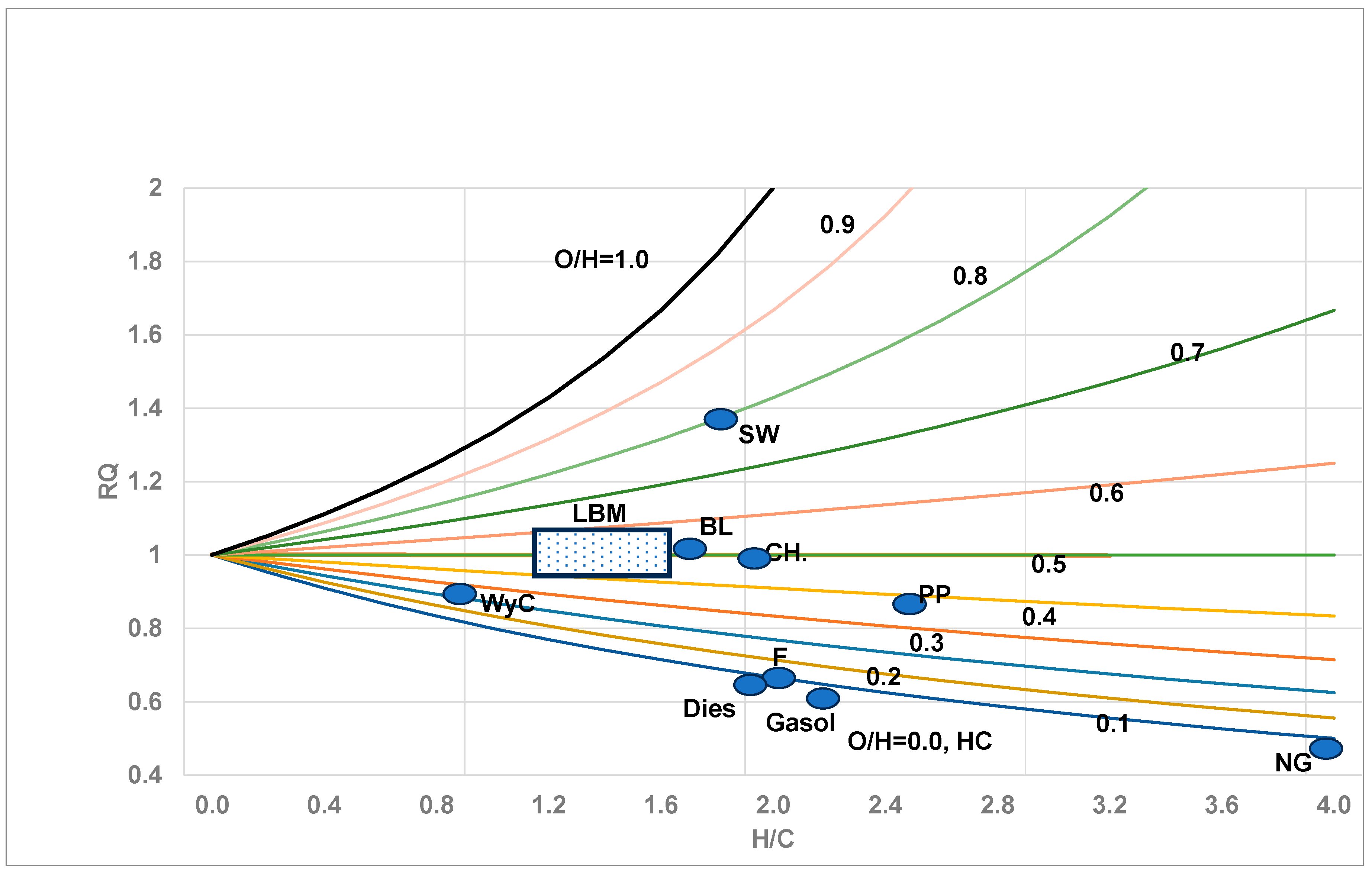
The RQ concept was applied to fossil fuels (FFs) fired for power plants [45], and the relation between RQ and CO₂ released in GT per Exa J was presented:

$$C{O}_2,\left(\frac{GT}{ExaJ}\right)=\frac{M_{CO2}}{HH{V}_{O2}}RQ={ \mathrm{F}}_{CO2EJ}\ast RQ ,{\mathrm{F}}_{CO2EJ}=\frac{M_{CO2}}{HH{V}_{O2}}\approx 0.1$$

(3)

where HHV_O2 = 448 Exa J/Peta mole of O₂, and M_CO2 = 44.01 g/mole or 44.01 GT per Peta mole of CO₂.

(v)

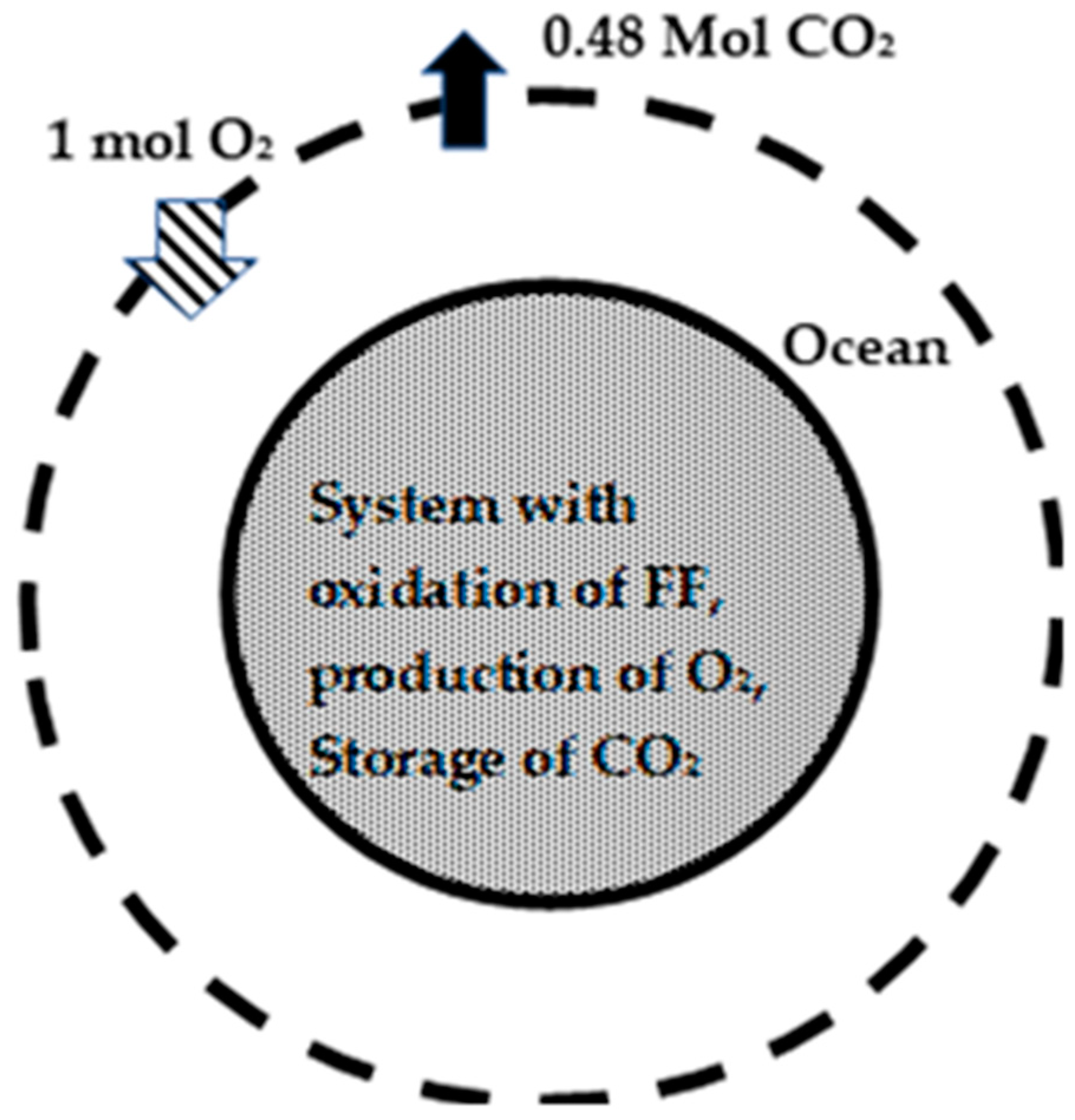
The Keeling’s data [46] on CO₂ and O₂ were used to obtain curve fit constants using linear and quadratic fits and present RQ_Glob as 0.47 (=d(CO₂)/dt) in the atmosphere/ |d(O₂)/dt| in the atmosphere), which is similar to ARQ in biology. Planet Earth behaves like a large BS, releasing 0.47 moles of CO₂ to the atmosphere for every mole of O₂ depleted from the atmosphere. The RQ_Glob is much less than the RQ of FFs due to CO₂ sink by biomass and CO₂ storage in the oceans.

(vi)

It was shown that the global RQ_Glob is a measure of the acidity of the oceans [9]. The lower the RQ_Glob is and the larger the difference between RQ_FF and RQ_Glob, the greater the acidity of the oceans.

Figure 1. Variation in RQ (CH_hO_o fuel or nutrients with (h = H/C, o = O/C), with O/H as parameter. Generally, RQ = 1/ (1 + h/4 − o/2) or 1/ [1 + (h/4) * {1 − 2 * (O/H)}] At O/H = 0.5, RQ = 1. Figure adopted from [47] and modified. Symbols denote RQ estimated from chemical formula of many fuels and nutrients. Most land biomasses have O/H varying from 0.4 (Table A.1 in Appendix of Part I) to 0.57 with an average of 0.49 (see rectangular box labelled LBM), while RQ _LBM varies from 0.94 to 1.05 with an average of around 1 due to O/H = 0.5; see horizontal line. It appears as though H₂O molecule is chemically attached to C atom in the BM when O/H = 0.5 and hence, during oxidation, H₂O is detached, O₂ is needed to oxidize only C, and as such, RQ = 1; during growth of biomass, C is separated from CO₂ and again RQ_LBM = 1.

Figure 1. Variation in RQ (CH_hO_o fuel or nutrients with (h = H/C, o = O/C), with O/H as parameter. Generally, RQ = 1/ (1 + h/4 − o/2) or 1/ [1 + (h/4) * {1 − 2 * (O/H)}] At O/H = 0.5, RQ = 1. Figure adopted from [47] and modified. Symbols denote RQ estimated from chemical formula of many fuels and nutrients. Most land biomasses have O/H varying from 0.4 (Table A.1 in Appendix of Part I) to 0.57 with an average of 0.49 (see rectangular box labelled LBM), while RQ _LBM varies from 0.94 to 1.05 with an average of around 1 due to O/H = 0.5; see horizontal line. It appears as though H₂O molecule is chemically attached to C atom in the BM when O/H = 0.5 and hence, during oxidation, H₂O is detached, O₂ is needed to oxidize only C, and as such, RQ = 1; during growth of biomass, C is separated from CO₂ and again RQ_LBM = 1.

2.7. Objectives of Part II

The objectives of Part II are as follows: (i) Present CO₂ (or C) and O₂ balance equations, (ii) obtain solutions for global O₂ production by land and ocean-based biomasses and CO₂ storage by the ocean, (iii) define energy-based RQ_Glob(En) and estimate it using the curve fit constants for Keeling’s curve (linear and quadratic curve fits), (iv) provide explicit formulae for the CO₂ distribution in GT/year and % contribution amongst the atmosphere, land biomass (LBM), and ocean water biomass (OWBM) and the amount stored in ocean water (St, Ocn), (v) validate the results from the RQ method by comparing them with the literature results obtained from more detailed numerical models, which are presented in Global Carbon Project (GCP) reports, and (vi) relate the rate of global temperature rise in terms of RQ_Glob(En) and annual energy release rate from FFLU.

3. Materials and Methods

3.1. Assumptions

• Humans and land and ocean-based animals consume renewable energy (not coal, oil, or fossil fuels), which presumes that the CO₂ produced and O₂ consumed by humans and animals is approximately equal to the CO₂ sink and O₂ production in growing “nutrient-crops”; they operate on “closed C” loop.
• Biomass includes terrestrial (land) and ocean water-based or marine biomass and micro-organisms.
• CO₂ is released during calcination (cement making without using oxygen), and CO₂ is used in limestone formations in the ocean (without the use of O₂). It can be accounted for through the definition of an effective RQ_OWBM. Note that the C(s) from calcination (cement carbonation) is only 0.2 GT of C/year, while the CO₂ storage in the ocean is 90 GT of C/year.
• While CO₂ is stored, there is no net O₂ storage in the oceans; there was only a 2% drop in ocean’s oxygen levels over the last 50 years [48], and hence, O₂ storage in OW is neglected compared to CO₂ since O₂ in the atmosphere is at much higher concentrations and the ocean is nearly saturated with O₂ due to much higher concentrations of O₂ in the atmosphere compared to CO₂ (note: solubility CO₂: 0.0116 mL per L per mm Hg, O₂: 0.00565 mL/L per mm Hg; typically, O₂ saturation level in OW is about 7–8 mg/L, CO₂ 0.44–0.66 mg for warm to cold water; O₂ saturation level is high due to the high concentration of O₂ in the atmosphere}).
• Changes in O₂ and CO₂ storage due to changes in the temperature of ocean water are ignored in CO₂ and O₂ balance equations.

Additional assumptions, if any, are stated as the governing equations are presented.

3.2. CO₂ and O₂ Balance Equations and Solutions for CO₂ Distribution amongst Atmosphere, Land, and Ocean

(i)

CO₂ Balance Equations

The C emissions are from fossil fuels via CO₂ (CE_FF), and cement production and land use (CE_LU), and C sinks are in land biomass (CS_LBM) due to the fertilization of plants on land and ocean biomasses (CS _OWBM), storage of CO₂ in the atm [44] (CS_ATM), and storage in the ocean water (CS_St,_Ocn, i.e., without O₂ production) as dissolved gas and as carbonate.

The C atom balance equation is written as follows:

$$\mathrm{Catom}:\left\{{(\mathrm{C}\mathrm{E})}_{\mathrm{F}\mathrm{F}}+{(\mathrm{C}\mathrm{E})}_{\mathrm{L}\mathrm{U}}\right\}=\left\{{(\mathrm{C}\mathrm{S})}_{\mathrm{A}\mathrm{t}\mathrm{m}}+{(\mathrm{C}\mathrm{S})}_{\mathrm{L}\mathrm{B}\mathrm{M}}+{(\mathrm{C}\mathrm{S})}_{\mathrm{O}\mathrm{W}\mathrm{B}\mathrm{M}}+{(\mathrm{C}\mathrm{S})}_{\mathrm{S}\mathrm{t},\mathrm{O}\mathrm{c}\mathrm{n}}\right\}$$

(4)

which can be equally applied to CO₂ since 1 mole of CO₂ contains 1 mole of carbon. Replacing C with CO₂ in Equation (4) and solving for the CO₂ storage rate in the atmosphere yields the following:

$${\left\{\frac{d\left[C{O}_2\right]}{dt}\right\}}_{atm}\ast {10}^{-06}\ast N_{air}\approx \left\{{\dot{N}}_{CO2,FFLU}-{\dot{N}}_{CO2,LOWBM}-{\dot{N}}_{CO2,st,Ocn}\right\}$$

(5)

where ${\dot{N}}_{CO2,FFLU}={\dot{N}}_{CO2,FF}+{\dot{N}}_{CO2,LU},{\dot{N}}_{CO2,LOWBM}={\dot{N}}_{CO2,LBM}+{\dot{N}}_{CO2,OWBM}$, ${\left\{\frac{d\left[C{O}_2\right]}{dt}\right\}}_{atm}$ is the accumulation rate of CO₂ in the atmosphere, ppm/year, N_air is the atmosphere air, in Peta moles, ${\dot{N}}_{CO2,FF}$ and ${\dot{N}}_{CO2,LU}$ are the annual CO₂ release rates by FFs and LU, ${\dot{N}}_{CO2,FFLU}$ is the combined CO₂ from FFs and LU, ${\dot{N}}_{CO2,LBM}$ is the CO₂ sink via land biomass, ${\dot{N}}_{CO2,OWBM}$ is the CO₂ sink via ocean water-based biomass, ${\dot{N}}_{CO2,LOWBM}$ is the combined CO₂ sink via land and ocean water-based biomasses and ${\dot{N}}_{CO2,st,Ocn}$ is the CO₂ storage by the oceans, and all rates are in Peta moles/year. Appendix A shows the conversion from ppm of species per year to GT per year.

(ii)

O₂ Balance Equation: see Huang et al. [25]:

$$\begin{array}{l}{\left\{\frac{d[O_2]}{dt}\right\}}_{atm}\ast {10}^{-6}{N}_{air}\approx -{\dot{N}}_{O2,FFLU}+{\dot{N}}_{O2,LOWBM}\\ {\dot{N}}_{O2,FFLU}={\dot{N}}_{O2,FF}+{\dot{N}}_{O2,LU},{\dot{N}}_{O2,LOWBM}={\dot{N}}_{O2,LBM}+{\dot{N}}_{O2,OWBM},{\dot{N}}_{O2,FFLU}=\frac{{\dot{E}}_{FFLU}}{HHVO2}\end{array}$$

(6)

where ${\left\{\frac{d\left[O_2\right]}{dt}\right\}}_{atm}$ is the yearly depletion rate of O₂ in the atmosphere, in ppm/year, ${\dot{N}}_{O2,FF}$, and ${\dot{N}}_{O2,LU}$ are the annual O₂ consumption rates by FFs and LU, ${\dot{N}}_{O2,FFLU}$ is the combined O₂ consumed by FFs and LU and is estimated from annual data on energy released by FF and LU, {${\dot{E}}_{FFLU}$}, ${\dot{N}}_{O2,LBM}$ is the O₂ production rate via land biomass, ${\dot{N}}_{O2,OWBM}$ is the O₂ production rate via ocean water-based biomass (e.g., PP), ${\dot{N}}_{O2,LOWBM}$ is the combined O₂ production rate via land and ocean water biomasses after accounting for the cost of respiration by plants and microbial decomposition. It is noted that the oxygen consumed by FFLU ${\dot{N}}_{O2,FFLU}$ is proportional to energy released by FFLU by various fuel types and as such, % oxygen consumed by each fuel type is the same as % energy released by each fuel type; thus, the energy % (2022) or O₂% consumed by gas, coal, and oil is 28.7%, 32.7%, and 38.6% [49].

(iii)

CO₂ Source/Sink in Atmosphere in terms of RQ

Using the definition of RQ, the CO₂ balance Equation (5) becomes

$$\begin{array}{l}{\left\{\frac{d\left[C{O}_2\right]}{dt}\right\}}_{atm}\ast {10}^{-06}\ast N_{air}\approx \left\{R{Q}_{FFLU}{\dot{N}}_{O2,FFLU}-R{Q}_{LOWBM}{\dot{N}}_{O2,LOWBM}-{\dot{N}}_{CO2,st,Ocn}\right\}\\ R{Q}_{FFLU}{\dot{N}}_{O2,FFLU}=R{Q}_{FF}{\dot{N}}_{CO2,FF}+R{Q}_{LU}{\dot{N}}_{O2,LU},R{Q}_{LOWBM}{\dot{N}}_{O2,LOWBM}=R{Q}_{LBM}{\dot{N}}_{O2,LBM}+R{Q}_{OWBM}{\dot{N}}_{O2,OWBM}\end{array}$$

(7)

Dividing by ${\dot{N}}_{O2,FFLU}$, and defining the energy-based RQ_Glob(En) as

$$R{Q}_{Glob(En)}=\frac{{\left\{\frac{d(\left[C{O}_2\right]}{dt}\right\}}_{atm}\left({10}^{-6}\ast N_{air}\right)}{{\dot{N}}_{O2,FFLU}}=\frac{{\left\{\frac{d\left[C{O}_2\right]}{dt}\right\}}_{atm}\ast F_{Bal}}{{\dot{E}}_{FFLU}}$$

(8)

the dimensionless form of Equation (7) is written as

$$R{Q}_{Glob(En)}=\left\{\frac{{\left\{\frac{d\left[C{O}_2\right]}{dt}\right\}}_{atm}}{{\dot{N}}_{O2FFLU}}\right\}\ast N_{air}\ast {10}^{-6}=R{Q}_{FFLU}-x\ast R{Q}_{LOWBM}-y$$

(9)

or

$$R{Q}_{Glob(En)}=\left\{\frac{{\left\{\frac{d\left[C{O}_2\right]}{dt}\right\}}_{atm}}{{\dot{E}}_{FFLU}}\right\}\ast F_{Bal}=R{Q}_{FFLU}-x\ast R{Q}_{LOWBM}-y,F_{Bal}=HH{V}_{O2}\ast N_{air}\ast {10}^{-6}=79.3$$

(10)

where R_Glob(en) definition is presented in column 2 and row (6a), of Table 2 and typical values for RQ_FF, RQ_LU, etc. are presented in Table 3. The definition for F_Bal along with their values are presented in Table 4.

$$x=\frac{{\dot{N}}_{O2,LOWBM}}{{\dot{N}}_{O2,FFLU}}$$

(11)

$$y=\frac{{\dot{N}}_{CO2,st,ocn}}{{\dot{N}}_{O2,FFLU}}=R{Q}_{FFLU}\frac{{\dot{N}}_{CO2,st,ocn}}{{\dot{N}}_{CO2,FFLU}}$$

(12)

$$R{Q}_{FFLU}=R{Q}_{FF}\ast E{F}_{FF}+R{Q}_{LU}\ast E{F}_{LU},E{F}_{FF}=\frac{{\dot{N}}_{O2,FF}}{{\dot{N}}_{O2,FFLU}},E{F}_{LU}=\frac{{\dot{N}}_{O2,LU}}{{\dot{N}}_{O2,FFLU}}$$

(13)

Further,

$$R{Q}_{LOWBM}=\frac{{\dot{N}}_{CO2,LOWBM}}{{\dot{N}}_{O2,LOWBM}}=R{Q}_{LBM}\ast (1-z)+R{Q}_{OWBM}\ast z$$

(14)

where

$$z=\frac{{\dot{N}}_{O2,OWBM}}{{\dot{N}}_{O2,LOWBM}},1-z=\frac{{\dot{N}}_{O2,LBM}}{{\dot{N}}_{O2,LOWBM}}$$

(15)

where EF, the Energy fraction contribution by FFs, LU, and z, is a measure of the fraction of oxygen contributed by OWBM to the atm. More discussion on the values of “z” will be given later in Section 4.4.1.

Note that soil absorbs roughly 25% of anthropogenic emissions each year and is stored in peatland or permafrost without a well-defined release of O₂; this can be accounted for by altering RQ_LBM and RQ_OWBM; see Refs. [27,28].

3.3. Solutions for O₂ Production, CO₂ Storage in Ocean, and Carbon Budget

Solutions for O₂ Production and CO₂ Storage in Ocean

The CO₂ and O₂ balance equations indicate that the atmospheric O₂ and CO₂ in the Keeling curve are affected by O₂ consumption and CO₂ production via FFLU, O₂ production, and CO₂ sink by land and ocean biomasses and ocean storage. Thus, the two equations (Equations (6) and (7)) can be solved for two unknowns: O₂ production by biomass, ${\dot{N}}_{O2,LOWBM}$, and CO₂ storage by ocean, ${\dot{N}}_{CO2,st,Ocn}$. Appendix B presents the normalization of Equations (9) and (10) and describes the solution procedure. The solutions for the non-dimensional form of O₂ production rate (x) and CO₂ storage rate (y) are obtained and presented in Rows 7 and 10 of Table 2. It also lists a summary of all the solutions. Note that “y” is not RQ even though both are ratios of CO₂ to O₂.

Rows 1 and 2: Curve Fit Constants for CO₂ and O₂.

Rows 3a and 3b: Slopes of CO₂ in ppm/year and GT/year.

Rows 4a and 4b: Slopes of O₂ in ppm/year and GT/year.

Rows 7 and 10: Solutions for “x” and “y”.

The net O₂ moles transferred by ocean and land biomasses to the atmosphere per unit of O₂ consumed by FFLU are given as

$$\frac{{\dot{N}}_{O_2,OWBM}}{{\dot{N}}_{O_2,FFLU}}=z\ast x$$

(16)

$$\frac{{\dot{N}}_{O_2,LBM}}{{\dot{N}}_{O_2,FFLU}}=(1-z)\ast x,$$

(17)

See Rows 8 and 9 in Table 2 for the O₂ contribution by ocean and land biomasses.

3.4. Global RQ_Glob and Energy-Based RQ_Glob(En)

Global RQ: Part I [9] defined RQ _Glob as follows (Column 2, Row 5 of Table 2):

$$R{Q}_{Glob}=\frac{{\left\{\frac{d\left[C{O}_2\right]}{dt}\right\}}_{atm}}{{\left|\frac{d\left[O_2\right]}{dt}\right|}_{atm}}$$

(18)

where d[CO₂]/dt is the addition rate of CO₂ to the atmosphere. Both CO₂ and O₂ slopes are known from Keeling’s data and in terms of curve fit constants.

Energy-based RQ_Glob(En): Definition is given in Equations (8) and (10). If energy data are not available for the year of interest (i.e., 2006) and instead, C data are available in GT/year, then C in Peta Moles per year = {C(s) in GT per year/12.01}, which is the same as CO₂ in Peta Moles/year. Then the required O₂ in Peta moles is given as {CO₂ in Peta moles per year/ RQ_FFLU}.

Table 2. List of formulae for estimation of global respiratory quotient of planet, CO₂ distribution amongst the atmosphere, land biomass (LBM), ocean water biomass (OWBM), and ocean water storage (St, On). For list of “F” values in many relations, see Table 4. For data on constants a₀, a₁… j₀, j₁, see Section 3.4.2. Unless otherwise stated, most of the results on CO₂ budget are energy-based. For the year 2006, the quantitative numbers generated by the current method are in curly brackets { }, while the reported data are in square brackets [ ]. Unless otherwise stated, the GT per year denotes GT of CO₂ per year.

#	Variable	Linear Fit Numbers for 2006 in Parenthesis {}	Quadratic Fit (Also Called Parabolic Fit) Numbers for 2006 in Parenthesis { }
	Curve Fit Constants and Slopes of Keeling’s curves on CO2 and O2
1	Linear Fit of Keeling’s curve: CO2 in atmosphere, ppm	a1 * years + a0, linear fit {Est. CO2 for year 2006 = 381.7 ppm} [Keeling’s data 382.1 ppm]	c2 * years2 + c1 * years + c0, {CO2 for year 2006 = 380.5 ppm} [Keeling’s data 382.1 ppm]
2	O2 in atmosphere ppm	b1 * years + b0 {Est O2 for year 2006 = 209421.4 ppm} [Keeling’s data: 209,423 ppm]	d2 * years2 + d1 * years + d0,d2 = −0.0435 ppm/year2, d1 = −3.0332 ppm/year, {Est O2 for year 2006 = 209,424.6 ppm} [Keeling’s data: 209,423]
3a	d[CO2]/d(year) = CO2 change per year, ppm in atmosphere /year	a1 {2.081 ppm/year, constant, independent of year}	2 * c2 * years + c1 {2.04 ppm/year in 2006}
3b	d (CO2)/d(year), GT/year 1 ppm of CO2 in atmosphere = 7.79 GT	7.79 * a1 {16.2 in 2006, independent of year} [13.7 in 2006, 7% imbalance]	7.79 * 2 * c2 * years + c1 {15.9 in 2006} [13.7 in 2006, 7% imbalance]
4a	d[O2]/d(year), ppm/year 1 ppm of O2 in atmosphere = 5.66 GT	b1, negative {−4.44 ppm/year, constant, independent of year}	2 * d2 * years + d1 {−4.34 ppm/year in 2006}
4b	d(O2)/d(year)dO2/dt, GT removed from atmosphere/year	5.66 |b1|, b1 in ppm/year {25.12 GT/year, constant and independent of year}	$\left|\left(15.58\ast d_2\ast year+7.79\ast d_1\right)\right|$ {24.59 GT/year in 2006}
Global RQ
5	$R{Q}_{Glob}=\frac{{\left(\frac{d\left[C{O}_2\right]}{dt}\right)}_{atm}}{\left|{\left(\frac{d\left[O_2\right]}{dt}\right)}_{atm}\right|}$	$\frac{{\mathrm{a}}_1}{\left|{\mathrm{b}}_1\right|}$, constant {0.468 constant, independent of year}	$\left(\frac{2\ast {\mathrm{c}}_2\ast \mathrm{y}\mathrm{e}\mathrm{a}\mathrm{r}+{\mathrm{c}}_1}{\left|2\ast {\mathrm{d}}_2\ast \mathrm{y}\mathrm{e}\mathrm{a}\mathrm{r}+{ \mathrm{d}}_1\right|}\right)$, decreases slightly with years, {0.470 in 2006}
6a	$R{Q}_{Glob(En)}=\frac{{\left(\frac{d\left[C{O}_2\right]}{dt}\right)}_{atm}\ast \left({10}^{-6}\ast N_{air}\right)}{{\dot{N}}_{O2,FFLU}}$ With Energy data, {d[CO2]/dt}, ppm/year	$\frac{F_{Bal}\ast a_1}{{\dot{E}}_{FFLU}}=R{Q}_{Glob,}\ast \left\{\frac{F_{Bal}\ast b_1}{{\dot{E}}_{FFLU}}\right\},$ ${\dot{E}}_{FFLU}$ in Exa J/Year, a1, b1, ppm/year, FBal = 79.3 (see Table 4 for FBal relation) {0.358 in 2006}	$\begin{array}{l}\frac{F_{Bal}\ast \left(2\ast c_2\ast year+c_1\right)}{{\dot{E}}_{FFLU}},\\ R{Q}_{Glob,}\ast \left\{\frac{F_{Bal}\ast \left|\left(2\ast d_2\ast years+d_1\right)\right|}{{\dot{E}}_{FFLU}}\right\}\end{array}$ ${\dot{E}}_{FFLU}$ in Exa J/Year, a1, b1, ppm/year {0.352 in 2006}
6b	$R{Q}_{Glob(En)}=\frac{{\left(\frac{d\left[C{O}_2\right]}{dt}\right)}_{atm}\ast \left({10}^{-6}\ast N_{air}\right)}{{\dot{N}}_{O2,FFLU}}$ With C data in GT/year, {d[CO2]/dt}, ppm/year	$\frac{F_{CGt}\ast a_1}{\left({\dot{C}}_{FFLU}/R{Q}_{FFLU}\right)}=R{Q}_{Glob,}\ast \left\{\frac{F_{CGt}\ast b_1}{{\dot{E}}_{FFLU}}\right\}$ (see Table 4 for FCGt relation) FCGt = 2.13, in GT/Year, a1, b1, ppm/year, {0.36 in 2006}	$\begin{array}{l}\frac{F_{CGt}\ast \left(2\ast c_2\ast year+c_1\right)\ast R{Q}_{FFLU}}{{\dot{C}}_{FFLU}},\\ R{Q}_{Glob,}\ast \left\{\frac{F_{CGt}\ast \left|\left(2\ast d_2\ast years+d_1\right)\right|\ast R{Q}_{FFLU}}{{\dot{C}}_{FFLU}}\right\}\end{array}$ ${\dot{C}}_{FFLU}$ in GT/Year, a1, b1, ppm/year, {0.36 in 2006}
6c	$R{Q}_{Glob(En)}=\frac{{\left(\frac{d\left[C{O}_2\right]}{dt}\right)}_{atm}\ast \left({10}^{-6}\ast N_{air}\right)}{{\dot{N}}_{O2,FFLU}}$ {d[CO2]/dt}, ppm/year	$\frac{{\left(\frac{d\left[CO2\right]}{dt}\right)}_{atm}}{F_{CO2}{\dot{E}}_{FFLU}}$, $F_{CO2}=0.0126$	$\frac{{\left(\frac{d\left[CO2\right]}{dt}\right)}_{atm}}{F_{CO2}{\dot{E}}_{FFLU}}$ FCO2 = 0.0126
Non-Dimensional Solutions for O2 Production and CO2 Storage in Ocean
7a	$x=\frac{{\dot{N}}_{O2,LOWBM}}{{\dot{N}}_{O2,FFLU}},$	$\left\{1-\frac{F_{Bal}\ast \left|b_1\right|}{{\dot{E}}_{FFLU}}\right\}$, FBal = 79.3 {0.24 in year 2006 with FFLU Energy/year =460.1 Exa J/year}	$\left\{1-\frac{F_{Bal}\ast \left|\left(2\ast d_2\ast years+d_1\right)\right|}{{\dot{E}}_{FFLU}}\right\}$ {0.25 in year 2006}
7b	$x=\frac{{\dot{N}}_{O2,LOWBM}}{{\dot{N}}_{O2,FFLU}},$ With C data	$x=1-\left\{\frac{F_{CGt}\ast \left|b_1\right|\ast R{Q}_{FFLU}}{{\dot{C}}_{FFLU}}\right\},F_{CGt}=2.13$ ${\dot{C}}_{FFLU}$, carbon output GT/year by FFLU {0.24 with C data of 9.71 GT/year in 2006}	$x=1-\left\{\frac{F_{CGt}\ast \left|\left(2\ast d_2\ast years+d_1\right)\right|\ast R{Q}_{FFLU}}{{\dot{C}}_{FFLU}}\right\},F_{CGt}=2.13$ {0.26 in 2006}
7c	Total O2 prod GT/year, LOWBM Combined Ocean and land biomasses	FO2BM * x * ${\dot{E}}_{FFLU}$ FO2BM = 0.0714 {7.72 GT/year in 2006 with x = 0.235}	FO2BM * x * ${\dot{E}}_{FFLU}$, FO2BM = 0.0714 {8.25 GT/year in 2006 with x = 0.2516}
8	Ocean BM Contrib. O2 $\frac{{\dot{N}}_{O2,OWBM}}{{\dot{N}}_{O2,FFLU}}$	z * x, where x for linear fit {0.024 in 2006 with z = 0.1}	z * x, where x for quadratic fit {0.025 in 2006 with z = 0.1}
9	Land BM Contrib. O2 $\frac{{\dot{N}}_{O2,LBM}}{{\dot{N}}_{O2,FFLU}}$	(1 − z) * x {0.21 in 2006 with z = 0.1}	(1 − z) * x, where x for quadratic fit {0.23 in 2006 with z = 0.1}
10	CO2 storage $y=\frac{{\dot{N}}_{CO2,st,Ocn}}{{\dot{N}}_{O2,FFLU}}$	$y=R{Q}_{FFLU}-R{Q}_{LOWBM}\ast x-R{Q}_{Glob(En)}$ Or $R{Q}_{FFLU}-R{Q}_{LOWBM}+\frac{\left|b_1\right|\ast F_{Bal}\ast \left\{R{Q}_{LOWBM}-R{Q}_{Glob}\right\}}{{\dot{E}}_{FFLU}}$ {0.187}	$y=R{Q}_{FFLU}-R{Q}_{LOWBM}\ast x-R{Q}_{Glob(En)}$ Or $R{Q}_{FFLU}-R{Q}_{LOWBM}+\frac{\left|\left(2\ast d_2\ast years+d_1\right)\right|\ast F_{Bal}\ast \left\{R{Q}_{LOWBM}-R{Q}_{Glob}\right\}}{{\dot{E}}_{FFLU}}$ {0.178}
CO2 Budget Amongst Atmosphere, Land, and Ocean
11	$CO{2}_{Fr,atm}=\frac{{\dot{N}}_{CO2,atm}}{{\dot{N}}_{CO2,FFLU}}$	$\frac{a_1\ast F_{Bal}}{{\dot{E}}_{FFLU}\ast R{Q}_{FFLU}}or\frac{R{Q}_{Glob(En)}}{R{Q}_{FFLU}}$ {0.46 in 2006}	$\frac{F_{Bal}\ast \left(2\ast c_2\ast year+c_1\right)}{{\dot{E}}_{FFLU}\ast R{Q}_{FFLU}}$ {0.45 in 2006 }
12	$CO{2}_{Fr,LOWBM}=\frac{{\dot{N}}_{CO2,LOWBM}}{{\dot{N}}_{CO2,FFLU}}$	$\frac{R{Q}_{LO1WBM}\ast x}{R{Q}_{FFLU}}$ {0.30 in 2006}	$\frac{R{Q}_{LO1WBM}\ast x}{R{Q}_{FFLU}}$ {0.32 in 2006 }
13	$CO{2}_{Fr,St,Ocn}=\frac{{\dot{N}}_{CO2,St,Ocn}}{{\dot{N}}_{CO2,FFLU}}$	$1-x\frac{R{Q}_{LOWBM}}{R{Q}_{FFLU}}-\left\{\frac{F_{Bal}\ast a_1}{R{Q}_{FFLU}\ast {\dot{E}}_{FFLU}}\right\}$, $\frac{y}{R{Q}_{FFLU}}$ {0.24 in 2006 with Energy data}	$1-x\frac{R{Q}_{LOWBM}}{R{Q}_{FFLU}}-\left\{\frac{F_{Bal}\ast \left(2\ast c_2\ast years+c_1\right)}{R{Q}_{FFLU}\ast {\dot{E}}_{FFLU}}\right\}$ {0.23 in 2006 with Energy data}
14	CO2 sink Fr via Ocean Biomass $\frac{{\dot{N}}_{CO2,OWBM}}{{\dot{N}}_{CO2,FFLU}}$	$\left(\frac{R{Q}_{OWBM}}{R{Q}_{FFLU}}\right)\ast z\ast x$, {0.030 in 2006}	$\left(\frac{R{Q}_{OWBM}}{R{Q}_{FFLU}}\right)z\ast x$ {0.032 in 2006 with z = −0.1}
15	CO2 sink Fr Ocean Total $\frac{{\dot{N}}_{CO2,StOcn}+{\dot{N}}_{CO2,OWBM}}{{\dot{N}}_{CO2,FFLU}}$	$\frac{y}{R{Q}_{FFLU}}+\left(\frac{R{Q}_{OWBM}}{R{Q}_{FFLU}}\right)\ast z\ast x$ or $1-\frac{R{Q}_{Glob(En)}}{R{Q}_{FFLU}}$ {0.27 in 2006 with z = 0.1} [0.25 in 2006]	$\frac{y}{R{Q}_{FFLU}}+\left(\frac{R{Q}_{OWBM}}{R{Q}_{FFLU}}\right)\ast z\ast x$ {0.26 in 2006 with z = −0.1} [0.25 in 2006]
16	CO2 sink Fr LBM $\frac{{\dot{N}}_{CO2LBM}}{{\dot{N}}_{CO2,FFLU}}$	$\left(\frac{R{Q}_{LBM}}{R{Q}_{FFLU}}\right)(1-z)\ast x$ {0.27 in 2006 with z = 0.1} [0.33 in 2006 from data]	$\left(\frac{R{Q}_{LBM}}{R{Q}_{FFLU}}\right)\ast (1-z)\ast x$ {0.29 in 2006 with z = 0.1} [0.33 in 2006 from data]
17	CO2 sink by land and ocean biomasses, GT/year	$R{Q}_{LOWBM}\ast M_{CO2}\ast \left\{\frac{{\dot{E}}_{FFLU}}{HH{V}_{O2}}-F_{ppm}\ast \left|b_1\right|\right\}$ {10.5 GT/year in 2006}	$R{Q}_{LOWBM}\ast M_{CO2}\ast \left\{\frac{{\dot{E}}_{FFLU}}{HH{V}_{O2}}-F_{ppm}\ast \left(\left|2\ast d_2\ast year+d_1\right|\right)\right\}$ {11.2 GT/year in 2006}
18	CO2 sink by ocean biomass, GT/year	z * CO2 sink by land and ocean biomasses in GT/year {1.05 GT/year in 2006 with z = −0.1} No previous data to compare	z * CO2 sink by land and ocean biomasses in GT/year {1.12 GT/year in 2006 with z = −0.1} No previous data to compare
19	CO2 sink by land biomass, GT/year	(1 − z) * CO2 sink by land and ocean biomasses in GT/year {9.45 GT/year in 2006 with z = −0.1} [11.06 GT/year in 2006] [28]	(1 − z) * CO2 sink by land and ocean biomasses in GT/year {10.08 GT/year in 2006 with z = −0.1} [11.06 GT/year in 2006] [28]
20	CO2 storage by ocean, GT/year	FCO2EJ * y * ${\dot{E}}_{FFLU}$, FCO2EJ = MCO2/HHVO2 = 0.1 {8.63 GT/year in 2006} [8.36 GT/year in 2006] [50]	FCO2EJ * y * ${\dot{E}}_{FFLU}$, FCO2EJ = MCO2/HHVO2 = 0.1 {8.21 GT/year} [8.36 (GT/year in 2006] [50]
Global Temperature and Earth’s Mass Loss
21a	Global Temperature, °C vs. year	g1 * (year − 1991) + g0.	-
21b	Global Temperature rise $\Delta T ,°\mathrm{C}$ vs. CO2 of atmosphere in ppm.	${ \mathrm{h}}_1 \left(\frac{[C{O}_2]}{{[C{O}_2]}_{0,atm}}\right)+{\mathrm{h}}_0 ,$ ${[C{O}_2]}_{0,atm}$= 355 ppm in 1991 {2006, T in °C = 12.17; Data 12.06 °C}	$\begin{array}{l}\Delta T ,°C={ \mathrm{h}}_1 \left(\frac{[C{O}_2]}{[C{O}_{2,0}]}\right)+{\mathrm{h}}_0 ,\\ {\mathrm{h}}_1=4.0,{\mathrm{h}}_0=-4.10,[C{O}_{2,0}]=354ppm,\end{array}$
22a	Rate of Temperature rise per year, dT/d(year) in terms of Keeling’s data $\frac{dT}{dt}=\frac{{\mathrm{h}}_1}{[C{O}_{2,0}]} {\left(\frac{d[C{O}_2]}{dt}\right)}_{atm}$ {d[CO2]/dt}, ppm/year, [CO2,0], ppm	$\frac{{\mathrm{h}}_1{a}_1}{[C{O}_{2,0}]} ,{\mathrm{h}}_1=4.0$ 4 * (a1/a0) {1995 to 2022), dT/year = 0.024 °C /year}	$\frac{{\mathrm{h}}_1\left(2\ast c_2\ast years+c_1\right)}{[C{O}_{2,0}]}$ Years = Year of interest—1991 {1995 to 2022, dT/year = 0.023 °C/year }
22b	Rate of Temperature rise per year, dT/d (year) Energy data	$F_{dTdt}\ast R{Q}_{Glob(En)}\ast {\dot{E}}_{FFLU},F_{dTdt}=1.44\times {10}^{-4}$	$F_{dTdt}\ast R{Q}_{Glob(En)}\ast {\dot{E}}_{FFLU},F_{dTdt}=1.44\times {10}^{-4}$
23	Earth’s mass Loss Rate, GT/year	FCGTE * RQGlob(En) * ${\dot{E}}_{FFLU}$, Alternate: FCGT * (d[CO2]/dt)qtm {4.42 GT/year, 2006}	FCGTE * RQGlob(En) * ${\dot{E}}_{FFLU}$, Alternate: FCGT * (d[CO2]/dt)qtm {4.34 GT/year, 2006}

Table 2. List of formulae for estimation of global respiratory quotient of planet, CO₂ distribution amongst the atmosphere, land biomass (LBM), ocean water biomass (OWBM), and ocean water storage (St, On). For list of “F” values in many relations, see Table 4. For data on constants a₀, a₁… j₀, j₁, see Section 3.4.2. Unless otherwise stated, most of the results on CO₂ budget are energy-based. For the year 2006, the quantitative numbers generated by the current method are in curly brackets { }, while the reported data are in square brackets [ ]. Unless otherwise stated, the GT per year denotes GT of CO₂ per year.

#	Variable	Linear Fit Numbers for 2006 in Parenthesis {}	Quadratic Fit (Also Called Parabolic Fit) Numbers for 2006 in Parenthesis { }
	Curve Fit Constants and Slopes of Keeling’s curves on CO2 and O2
1	Linear Fit of Keeling’s curve: CO2 in atmosphere, ppm	a1 * years + a0, linear fit {Est. CO2 for year 2006 = 381.7 ppm} [Keeling’s data 382.1 ppm]	c2 * years2 + c1 * years + c0, {CO2 for year 2006 = 380.5 ppm} [Keeling’s data 382.1 ppm]
2	O2 in atmosphere ppm	b1 * years + b0 {Est O2 for year 2006 = 209421.4 ppm} [Keeling’s data: 209,423 ppm]	d2 * years2 + d1 * years + d0,d2 = −0.0435 ppm/year2, d1 = −3.0332 ppm/year, {Est O2 for year 2006 = 209,424.6 ppm} [Keeling’s data: 209,423]
3a	d[CO2]/d(year) = CO2 change per year, ppm in atmosphere /year	a1 {2.081 ppm/year, constant, independent of year}	2 * c2 * years + c1 {2.04 ppm/year in 2006}
3b	d (CO2)/d(year), GT/year 1 ppm of CO2 in atmosphere = 7.79 GT	7.79 * a1 {16.2 in 2006, independent of year} [13.7 in 2006, 7% imbalance]	7.79 * 2 * c2 * years + c1 {15.9 in 2006} [13.7 in 2006, 7% imbalance]
4a	d[O2]/d(year), ppm/year 1 ppm of O2 in atmosphere = 5.66 GT	b1, negative {−4.44 ppm/year, constant, independent of year}	2 * d2 * years + d1 {−4.34 ppm/year in 2006}
4b	d(O2)/d(year)dO2/dt, GT removed from atmosphere/year	5.66 |b1|, b1 in ppm/year {25.12 GT/year, constant and independent of year}	$\left|\left(15.58\ast d_2\ast year+7.79\ast d_1\right)\right|$ {24.59 GT/year in 2006}
Global RQ
5	$R{Q}_{Glob}=\frac{{\left(\frac{d\left[C{O}_2\right]}{dt}\right)}_{atm}}{\left|{\left(\frac{d\left[O_2\right]}{dt}\right)}_{atm}\right|}$	$\frac{{\mathrm{a}}_1}{\left|{\mathrm{b}}_1\right|}$, constant {0.468 constant, independent of year}	$\left(\frac{2\ast {\mathrm{c}}_2\ast \mathrm{y}\mathrm{e}\mathrm{a}\mathrm{r}+{\mathrm{c}}_1}{\left|2\ast {\mathrm{d}}_2\ast \mathrm{y}\mathrm{e}\mathrm{a}\mathrm{r}+{ \mathrm{d}}_1\right|}\right)$, decreases slightly with years, {0.470 in 2006}
6a	$R{Q}_{Glob(En)}=\frac{{\left(\frac{d\left[C{O}_2\right]}{dt}\right)}_{atm}\ast \left({10}^{-6}\ast N_{air}\right)}{{\dot{N}}_{O2,FFLU}}$ With Energy data, {d[CO2]/dt}, ppm/year	$\frac{F_{Bal}\ast a_1}{{\dot{E}}_{FFLU}}=R{Q}_{Glob,}\ast \left\{\frac{F_{Bal}\ast b_1}{{\dot{E}}_{FFLU}}\right\},$ ${\dot{E}}_{FFLU}$ in Exa J/Year, a1, b1, ppm/year, FBal = 79.3 (see Table 4 for FBal relation) {0.358 in 2006}	$\begin{array}{l}\frac{F_{Bal}\ast \left(2\ast c_2\ast year+c_1\right)}{{\dot{E}}_{FFLU}},\\ R{Q}_{Glob,}\ast \left\{\frac{F_{Bal}\ast \left|\left(2\ast d_2\ast years+d_1\right)\right|}{{\dot{E}}_{FFLU}}\right\}\end{array}$ ${\dot{E}}_{FFLU}$ in Exa J/Year, a1, b1, ppm/year {0.352 in 2006}
6b	$R{Q}_{Glob(En)}=\frac{{\left(\frac{d\left[C{O}_2\right]}{dt}\right)}_{atm}\ast \left({10}^{-6}\ast N_{air}\right)}{{\dot{N}}_{O2,FFLU}}$ With C data in GT/year, {d[CO2]/dt}, ppm/year	$\frac{F_{CGt}\ast a_1}{\left({\dot{C}}_{FFLU}/R{Q}_{FFLU}\right)}=R{Q}_{Glob,}\ast \left\{\frac{F_{CGt}\ast b_1}{{\dot{E}}_{FFLU}}\right\}$ (see Table 4 for FCGt relation) FCGt = 2.13, in GT/Year, a1, b1, ppm/year, {0.36 in 2006}	$\begin{array}{l}\frac{F_{CGt}\ast \left(2\ast c_2\ast year+c_1\right)\ast R{Q}_{FFLU}}{{\dot{C}}_{FFLU}},\\ R{Q}_{Glob,}\ast \left\{\frac{F_{CGt}\ast \left|\left(2\ast d_2\ast years+d_1\right)\right|\ast R{Q}_{FFLU}}{{\dot{C}}_{FFLU}}\right\}\end{array}$ ${\dot{C}}_{FFLU}$ in GT/Year, a1, b1, ppm/year, {0.36 in 2006}
6c	$R{Q}_{Glob(En)}=\frac{{\left(\frac{d\left[C{O}_2\right]}{dt}\right)}_{atm}\ast \left({10}^{-6}\ast N_{air}\right)}{{\dot{N}}_{O2,FFLU}}$ {d[CO2]/dt}, ppm/year	$\frac{{\left(\frac{d\left[CO2\right]}{dt}\right)}_{atm}}{F_{CO2}{\dot{E}}_{FFLU}}$, $F_{CO2}=0.0126$	$\frac{{\left(\frac{d\left[CO2\right]}{dt}\right)}_{atm}}{F_{CO2}{\dot{E}}_{FFLU}}$ FCO2 = 0.0126
Non-Dimensional Solutions for O2 Production and CO2 Storage in Ocean
7a	$x=\frac{{\dot{N}}_{O2,LOWBM}}{{\dot{N}}_{O2,FFLU}},$	$\left\{1-\frac{F_{Bal}\ast \left|b_1\right|}{{\dot{E}}_{FFLU}}\right\}$, FBal = 79.3 {0.24 in year 2006 with FFLU Energy/year =460.1 Exa J/year}	$\left\{1-\frac{F_{Bal}\ast \left|\left(2\ast d_2\ast years+d_1\right)\right|}{{\dot{E}}_{FFLU}}\right\}$ {0.25 in year 2006}
7b	$x=\frac{{\dot{N}}_{O2,LOWBM}}{{\dot{N}}_{O2,FFLU}},$ With C data	$x=1-\left\{\frac{F_{CGt}\ast \left|b_1\right|\ast R{Q}_{FFLU}}{{\dot{C}}_{FFLU}}\right\},F_{CGt}=2.13$ ${\dot{C}}_{FFLU}$, carbon output GT/year by FFLU {0.24 with C data of 9.71 GT/year in 2006}	$x=1-\left\{\frac{F_{CGt}\ast \left|\left(2\ast d_2\ast years+d_1\right)\right|\ast R{Q}_{FFLU}}{{\dot{C}}_{FFLU}}\right\},F_{CGt}=2.13$ {0.26 in 2006}
7c	Total O2 prod GT/year, LOWBM Combined Ocean and land biomasses	FO2BM * x * ${\dot{E}}_{FFLU}$ FO2BM = 0.0714 {7.72 GT/year in 2006 with x = 0.235}	FO2BM * x * ${\dot{E}}_{FFLU}$, FO2BM = 0.0714 {8.25 GT/year in 2006 with x = 0.2516}
8	Ocean BM Contrib. O2 $\frac{{\dot{N}}_{O2,OWBM}}{{\dot{N}}_{O2,FFLU}}$	z * x, where x for linear fit {0.024 in 2006 with z = 0.1}	z * x, where x for quadratic fit {0.025 in 2006 with z = 0.1}
9	Land BM Contrib. O2 $\frac{{\dot{N}}_{O2,LBM}}{{\dot{N}}_{O2,FFLU}}$	(1 − z) * x {0.21 in 2006 with z = 0.1}	(1 − z) * x, where x for quadratic fit {0.23 in 2006 with z = 0.1}
10	CO2 storage $y=\frac{{\dot{N}}_{CO2,st,Ocn}}{{\dot{N}}_{O2,FFLU}}$	$y=R{Q}_{FFLU}-R{Q}_{LOWBM}\ast x-R{Q}_{Glob(En)}$ Or $R{Q}_{FFLU}-R{Q}_{LOWBM}+\frac{\left|b_1\right|\ast F_{Bal}\ast \left\{R{Q}_{LOWBM}-R{Q}_{Glob}\right\}}{{\dot{E}}_{FFLU}}$ {0.187}	$y=R{Q}_{FFLU}-R{Q}_{LOWBM}\ast x-R{Q}_{Glob(En)}$ Or $R{Q}_{FFLU}-R{Q}_{LOWBM}+\frac{\left|\left(2\ast d_2\ast years+d_1\right)\right|\ast F_{Bal}\ast \left\{R{Q}_{LOWBM}-R{Q}_{Glob}\right\}}{{\dot{E}}_{FFLU}}$ {0.178}
CO2 Budget Amongst Atmosphere, Land, and Ocean
11	$CO{2}_{Fr,atm}=\frac{{\dot{N}}_{CO2,atm}}{{\dot{N}}_{CO2,FFLU}}$	$\frac{a_1\ast F_{Bal}}{{\dot{E}}_{FFLU}\ast R{Q}_{FFLU}}or\frac{R{Q}_{Glob(En)}}{R{Q}_{FFLU}}$ {0.46 in 2006}	$\frac{F_{Bal}\ast \left(2\ast c_2\ast year+c_1\right)}{{\dot{E}}_{FFLU}\ast R{Q}_{FFLU}}$ {0.45 in 2006 }
12	$CO{2}_{Fr,LOWBM}=\frac{{\dot{N}}_{CO2,LOWBM}}{{\dot{N}}_{CO2,FFLU}}$	$\frac{R{Q}_{LO1WBM}\ast x}{R{Q}_{FFLU}}$ {0.30 in 2006}	$\frac{R{Q}_{LO1WBM}\ast x}{R{Q}_{FFLU}}$ {0.32 in 2006 }
13	$CO{2}_{Fr,St,Ocn}=\frac{{\dot{N}}_{CO2,St,Ocn}}{{\dot{N}}_{CO2,FFLU}}$	$1-x\frac{R{Q}_{LOWBM}}{R{Q}_{FFLU}}-\left\{\frac{F_{Bal}\ast a_1}{R{Q}_{FFLU}\ast {\dot{E}}_{FFLU}}\right\}$, $\frac{y}{R{Q}_{FFLU}}$ {0.24 in 2006 with Energy data}	$1-x\frac{R{Q}_{LOWBM}}{R{Q}_{FFLU}}-\left\{\frac{F_{Bal}\ast \left(2\ast c_2\ast years+c_1\right)}{R{Q}_{FFLU}\ast {\dot{E}}_{FFLU}}\right\}$ {0.23 in 2006 with Energy data}
14	CO2 sink Fr via Ocean Biomass $\frac{{\dot{N}}_{CO2,OWBM}}{{\dot{N}}_{CO2,FFLU}}$	$\left(\frac{R{Q}_{OWBM}}{R{Q}_{FFLU}}\right)\ast z\ast x$, {0.030 in 2006}	$\left(\frac{R{Q}_{OWBM}}{R{Q}_{FFLU}}\right)z\ast x$ {0.032 in 2006 with z = −0.1}
15	CO2 sink Fr Ocean Total $\frac{{\dot{N}}_{CO2,StOcn}+{\dot{N}}_{CO2,OWBM}}{{\dot{N}}_{CO2,FFLU}}$	$\frac{y}{R{Q}_{FFLU}}+\left(\frac{R{Q}_{OWBM}}{R{Q}_{FFLU}}\right)\ast z\ast x$ or $1-\frac{R{Q}_{Glob(En)}}{R{Q}_{FFLU}}$ {0.27 in 2006 with z = 0.1} [0.25 in 2006]	$\frac{y}{R{Q}_{FFLU}}+\left(\frac{R{Q}_{OWBM}}{R{Q}_{FFLU}}\right)\ast z\ast x$ {0.26 in 2006 with z = −0.1} [0.25 in 2006]
16	CO2 sink Fr LBM $\frac{{\dot{N}}_{CO2LBM}}{{\dot{N}}_{CO2,FFLU}}$	$\left(\frac{R{Q}_{LBM}}{R{Q}_{FFLU}}\right)(1-z)\ast x$ {0.27 in 2006 with z = 0.1} [0.33 in 2006 from data]	$\left(\frac{R{Q}_{LBM}}{R{Q}_{FFLU}}\right)\ast (1-z)\ast x$ {0.29 in 2006 with z = 0.1} [0.33 in 2006 from data]
17	CO2 sink by land and ocean biomasses, GT/year	$R{Q}_{LOWBM}\ast M_{CO2}\ast \left\{\frac{{\dot{E}}_{FFLU}}{HH{V}_{O2}}-F_{ppm}\ast \left|b_1\right|\right\}$ {10.5 GT/year in 2006}	$R{Q}_{LOWBM}\ast M_{CO2}\ast \left\{\frac{{\dot{E}}_{FFLU}}{HH{V}_{O2}}-F_{ppm}\ast \left(\left|2\ast d_2\ast year+d_1\right|\right)\right\}$ {11.2 GT/year in 2006}
18	CO2 sink by ocean biomass, GT/year	z * CO2 sink by land and ocean biomasses in GT/year {1.05 GT/year in 2006 with z = −0.1} No previous data to compare	z * CO2 sink by land and ocean biomasses in GT/year {1.12 GT/year in 2006 with z = −0.1} No previous data to compare
19	CO2 sink by land biomass, GT/year	(1 − z) * CO2 sink by land and ocean biomasses in GT/year {9.45 GT/year in 2006 with z = −0.1} [11.06 GT/year in 2006] [28]	(1 − z) * CO2 sink by land and ocean biomasses in GT/year {10.08 GT/year in 2006 with z = −0.1} [11.06 GT/year in 2006] [28]
20	CO2 storage by ocean, GT/year	FCO2EJ * y * ${\dot{E}}_{FFLU}$, FCO2EJ = MCO2/HHVO2 = 0.1 {8.63 GT/year in 2006} [8.36 GT/year in 2006] [50]	FCO2EJ * y * ${\dot{E}}_{FFLU}$, FCO2EJ = MCO2/HHVO2 = 0.1 {8.21 GT/year} [8.36 (GT/year in 2006] [50]
Global Temperature and Earth’s Mass Loss
21a	Global Temperature, °C vs. year	g1 * (year − 1991) + g0.	-
21b	Global Temperature rise $\Delta T ,°\mathrm{C}$ vs. CO2 of atmosphere in ppm.	${ \mathrm{h}}_1 \left(\frac{[C{O}_2]}{{[C{O}_2]}_{0,atm}}\right)+{\mathrm{h}}_0 ,$ ${[C{O}_2]}_{0,atm}$= 355 ppm in 1991 {2006, T in °C = 12.17; Data 12.06 °C}	$\begin{array}{l}\Delta T ,°C={ \mathrm{h}}_1 \left(\frac{[C{O}_2]}{[C{O}_{2,0}]}\right)+{\mathrm{h}}_0 ,\\ {\mathrm{h}}_1=4.0,{\mathrm{h}}_0=-4.10,[C{O}_{2,0}]=354ppm,\end{array}$
22a	Rate of Temperature rise per year, dT/d(year) in terms of Keeling’s data $\frac{dT}{dt}=\frac{{\mathrm{h}}_1}{[C{O}_{2,0}]} {\left(\frac{d[C{O}_2]}{dt}\right)}_{atm}$ {d[CO2]/dt}, ppm/year, [CO2,0], ppm	$\frac{{\mathrm{h}}_1{a}_1}{[C{O}_{2,0}]} ,{\mathrm{h}}_1=4.0$ 4 * (a1/a0) {1995 to 2022), dT/year = 0.024 °C /year}	$\frac{{\mathrm{h}}_1\left(2\ast c_2\ast years+c_1\right)}{[C{O}_{2,0}]}$ Years = Year of interest—1991 {1995 to 2022, dT/year = 0.023 °C/year }
22b	Rate of Temperature rise per year, dT/d (year) Energy data	$F_{dTdt}\ast R{Q}_{Glob(En)}\ast {\dot{E}}_{FFLU},F_{dTdt}=1.44\times {10}^{-4}$	$F_{dTdt}\ast R{Q}_{Glob(En)}\ast {\dot{E}}_{FFLU},F_{dTdt}=1.44\times {10}^{-4}$
23	Earth’s mass Loss Rate, GT/year	FCGTE * RQGlob(En) * ${\dot{E}}_{FFLU}$, Alternate: FCGT * (d[CO2]/dt)qtm {4.42 GT/year, 2006}	FCGTE * RQGlob(En) * ${\dot{E}}_{FFLU}$, Alternate: FCGT * (d[CO2]/dt)qtm {4.34 GT/year, 2006}

Table 3. RQ values selected for quantitative results.

Source or Sink of Interest	RQ
Fossil Fuels, FFs	0.75
Land Use, LU	1.0
Combined FFs and LU	EFFF * RQFF + EFLU * RQLU = 0.778
Land Biomass, LBM	1.0
Ocean water-based biomass, OWBM	0.87
Com Combined LBM + OWBM;	(1 − z) * RQLBM + (1 − z) * RQOWBM = 0.987 With z = 0.1

Table 3. RQ values selected for quantitative results.

Source or Sink of Interest	RQ
Fossil Fuels, FFs	0.75
Land Use, LU	1.0
Combined FFs and LU	EFFF * RQFF + EFLU * RQLU = 0.778
Land Biomass, LBM	1.0
Ocean water-based biomass, OWBM	0.87
Com Combined LBM + OWBM;	(1 − z) * RQLBM + (1 − z) * RQOWBM = 0.987 With z = 0.1

Table 4. The constants F: Relations and values. The subscripts for F indicate the “relations” where they were used, e.g., F_dTdt represents constants in the relation for dT/dt, etc.

Constants F	Relation	Value
FBal (item 6a, Table 2)	10−6 * Nair * HHVO2	79.3
FCGT (item 6b, Table 2)	FCGT = 10−6 * Nair * MC	2.13
FCEJ (item 7c, Table 2)	(MC/HHVO2)	0.0268
FCO2	$\left(\frac{{10}^6}{N_{air}\ast HH{V}_{O2}}\right)=\frac{1}{F_{Bal}}$	0.0126
FCO2EJ (item 20, Table 2)	$\frac{M_{CO2}}{HH{V}_{O2}}$	0.1
FO2BM (item 7c, Table 2)	$\frac{M_{O2}}{HH{V}_{O2}}$	0.0714
Fppm (item 17, Table 2)	10−6 * Nair	0.177
FdTdt (Equation (36))	$\left\{\frac{h_1\ast F_{CO2}}{\left[C{O}_{2,0}\right]}\right\}$	$1.44\times {10}^{-4}$, h1 = 4

Table 4. The constants F: Relations and values. The subscripts for F indicate the “relations” where they were used, e.g., F_dTdt represents constants in the relation for dT/dt, etc.

Constants F	Relation	Value
FBal (item 6a, Table 2)	10−6 * Nair * HHVO2	79.3
FCGT (item 6b, Table 2)	FCGT = 10−6 * Nair * MC	2.13
FCEJ (item 7c, Table 2)	(MC/HHVO2)	0.0268
FCO2	$\left(\frac{{10}^6}{N_{air}\ast HH{V}_{O2}}\right)=\frac{1}{F_{Bal}}$	0.0126
FCO2EJ (item 20, Table 2)	$\frac{M_{CO2}}{HH{V}_{O2}}$	0.1
FO2BM (item 7c, Table 2)	$\frac{M_{O2}}{HH{V}_{O2}}$	0.0714
Fppm (item 17, Table 2)	10−6 * Nair	0.177
FdTdt (Equation (36))	$\left\{\frac{h_1\ast F_{CO2}}{\left[C{O}_{2,0}\right]}\right\}$	$1.44\times {10}^{-4}$, h1 = 4

3.4.1. CO₂ Budget amongst Atmosphere, Land, and Ocean Biomasses and Ocean Storage

The solutions for CO₂ stored in the atmosphere, CO₂ sink by biomass, and CO₂ storage are presented in Appendix B. Appendix B provides the details of derivations.

Rows 11, 12, and 13: CO₂ stored in the atmosphere, CO₂ sink by biomass, and CO₂ storage in the ocean.

Rows 14 and 16: CO₂ stored in land biomass and ocean biomass.

Row 15: Combined CO₂ storage in the ocean and ocean biomass CO₂ stored in land biomass, ocean biomass.

Row 16: CO₂ fraction by land biomass.

Row 4b, and Rows 17–20 in GT/year for CO₂ sink in the atmosphere, combines land and ocean biomasses, ocean biomass, land biomass, and CO₂ stored in the ocean.

3.4.2. Data Used in Calculations

Input Data:

Curve fit constants.

Linear Fit [9]: d[CO₂]/dt = a₁ * years + a₀, d[O₂]/dt = b₁ * years + b₀, years = current year − 1991, linear fit a₀ = 350.5 ppm, a₁ = 2.081 ppm/year, R² = 0.97, and O₂ data, b₀ = 209488 ppm, b₁ = −4.438 ppm/year R² = 0.98.

Quadratic Fit [9]: d[CO₂]/dt = c₂ * years² + c₁ * years + c₀, d[O₂]/dt = d₂ * years² + d₁ * years + d₀, c₂ = 0.01892, c₁ = 1.473, c₀ = 354.1, R² = 0.98: O₂ data, d₀ = 209,480 ppm, d₁ = −3.0332 ppm/year, d₂ = −0.0435 ppm/year², R² = 0.99.

Global Average Temp vs. year, See Equation (31) and Row 21a of Table 2, g₀ = 13.7, g₁ = −5.281 * 10⁻³, g₂ = 9.114 * 10⁻⁵, R² = 0.90, years from 1880 to 2023.

Global Temp. See Equation (33) and Row 21b of Table 2, ΔT = T − T_0,91 vs. [CO₂]/[CO_2,0], h₁ = 4.0, h₀ = −4.10, R² = 0.86, [CO_2,0] = 355 ppm with 1991 data.

Global $\frac{{\dot{E}}_{FFLU}}{{\dot{E}}_{FFLU,0}}$ vs. $\frac{[C{O}_2]}{{[C{O}_2]}_0}$, See Equation (37) i₁ = 4.14, i₀ = −3.16, R² = 0.98.

Global $\frac{[C{O}_2]}{{[C{O}_2]}_0}$ vs. $\frac{{\dot{E}}_{FFLU}}{{\dot{E}}_{FFLU,0}}$. See Equation (37), j₁ = 0.24, j₀ = 0.76, R² = 0.98.

RQ’s: RQ_OWBM = 0.84, which is close to 0.86, suggested in [51].

RQ_FFLU = 0.78; compare with values in Ref. [52]: PQ = 1.1 or RQ_LBM = 0.91 for terrestrial plants [9].

O₂ Moles Consumed from FFLU Energy: $\left\{{\dot{N}}_{O2,FFLU}\right\}$ from energy data = $\frac{{\dot{E}}_{FFLU}}{HH{V}_{O2}}$

Atmosphere Properties:

Nair = 1.77 × 10⁵ Peta mol, Oxygen Concentration: 0.21 or 210,000 ppm.

One ppm of CO added to the atmosphere = 0.177 Peta moles of CO₂ added, 7.79 GT of CO₂ added to the atmosphere, or 2.12 GT of Carbon added to the atmosphere.

One ppm of O₂ removed from the atmosphere, 1 ppm = 0.177 Peta moles removed, or 5.66 GT of O₂ removed from the atmosphere.

C Imbalance % in literature data: 100 * {CO₂ source from FFLU − CO₂ sink in (atmosphere + land + ocean)}/FFLU CO₂

Adjustable parameter “z” (O₂ transferred from ocean to atmosphere/Total O₂ produced by LBM and OWBM.

2006 Data

$\left\{{\dot{E}}_{FFLU}\right\}$ = 408.25 (FF) + 51.96 (LU) = 460.21 Exa J; ${\dot{C}}_{FFLU}$ = 9.71 GT/year

LU energy = 11.3% of total energy from LU or 12.7% of FF energy

C (from FFLU) data in 2006: 9.71 GT/year or CO₂ data: 35.6 GT of CO₂ /year

$\left\{{\dot{N}}_{O2,FFLU}\right\}$ = 1.027 Peta moles /year.

3.4.3. Literature Results on CO₂ in Atmosphere, Land, and Ocean

Fossil and LU based CO₂ and energy data are from Ref. [50]. Atmosphere CO₂ data are from [53]. Ocean sink data are estimated from the average of several global ocean biogeochemistry models [44] and the ocean sink uncertainty of ±0.5 GT C/year. Land sink data are from the average of dynamic global vegetation models and uncertainty of ±0.9 GT C/year.

The C or CO₂ budget in literature is based on several “stand-alone” land and detailed ocean circulation models. The Global Carbon Budget (GCB) is published by the Global Carbon Project; a summary of various models is provided in [44]. The land sink for C is based on the average of global vegetation models [54]. The estimates on ocean storage are based on global ocean-atmosphere CO₂ flux using ocean surface CO₂ concentration gradients, satellite data, and an average of several global ocean biochemistry models.

4. Results and Discussion

Table 2 contains all necessary formulae for all the important results required in obtaining CO₂ distribution amongst the atmosphere, land, and ocean. The Supplemental Materials titled “Supp Step by Step CO₂ budget” describe the step-by-step procedure for obtaining the quantitative results for the year 2006 shown in Table 2 and most of the results presented in Section 4.1, Section 4.2, Section 4.3, Section 4.4 and Section 4.5. An Excel-based program was developed with input data from Section 3.4.2 and an output containing all the results for the variables is listed in Table 2. For 2006, computed numbers generated by the current method are shown in curly brackets {}, while the previous literature data obtained with more detailed models are presented within square brackets [ ] as the last line of each row in the third and fourth columns of Table 2.

(i) The results for the global respiratory quotients (RQ_Glob, RQ_Glob(En)), normalized O₂ production (“x”) and CO₂ storage (“y”), and energy released by FFLU vs. year will be presented first. (ii) The year 2006 was then selected for parametric studies since it was somewhere within the median year for data reported in 1991–2020 (30-year period), for which period the curve fits on Keeling’s data were obtained. (iii) The CO₂ in GT/year and % contributed by the atmosphere, land, and ocean storage will be f compared with previous data for 2006 with z as a parameter, and a suitable z value will be selected. For the year 2006, FFLU energy is reported as 460.2 Exa J and CO₂ emission is reported as 35.6 GT of CO₂ by FFLU. The RQ_FFLU is estimated at 0.78 (Part I) [9]. Typically, the more oxygen in FFs, the lesser the stoichiometric oxygen, the higher the RQ, and the higher the CO₂ emission per Exa J (Equation (3)). (iv) Then, using the selected z value, the annual RQ-based results on CO₂ distribution in the atmosphere, land, and ocean storage in GT/year and % vs. year for the years 1991 to 2018 will be compared with the previous data. (v) Based on current analysis, various methods of freezing CO₂ growth in atmosphere will be presented followed by presentation of relations between global temperature, rate of heating, Energy, and global CO₂ Concentration.

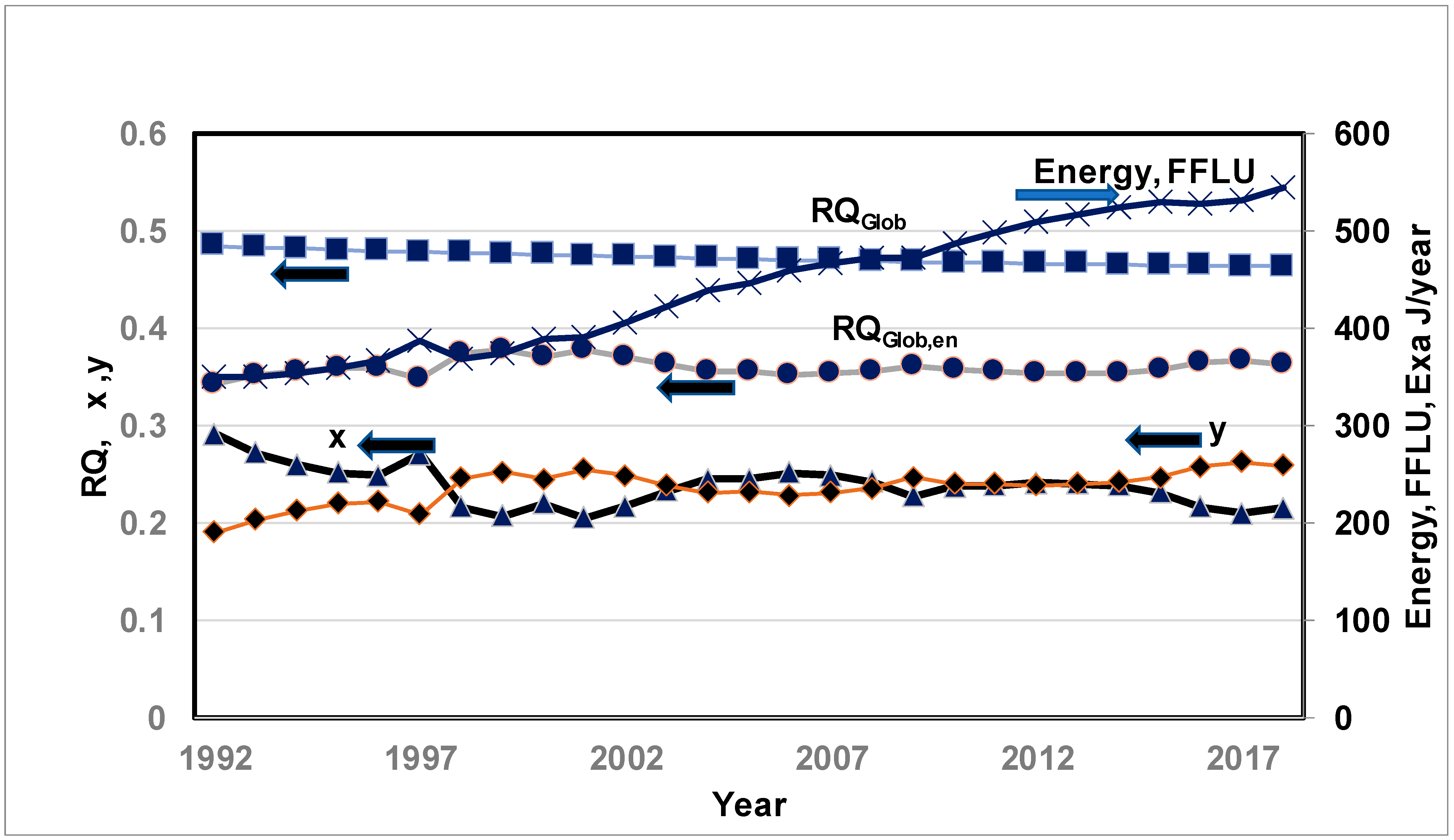
4.1. Global Respiratory Quotients (RQ_Glob, RQ_Glob(En))

Part I dealt with RQ_Glob, estimated as 0.47 using Keeling’s data (Row 5, Table 2) and remaining constant with linear fit. RQ_Glob decreases from 0.48 to 0.46 (1991–2020) for quadratic fit {part I, [9]} and RQ_Glob = 0.47 in 2006. It appears that Earth behaves like a large “Hypothetical Biological System (HBS)” (or “barren Earth” without chlorophyll and oceans) to sustain the lifelong activities of humans on Earth with the net effect of increasing CO₂ at the cost of decreasing O₂ in the atmosphere. For a linear fit on CO₂ data, the rate of increase in CO₂ is constant at 2.08 ppm/year, and the intercept on the Y-axis, i.e., CO₂ concentration in ppm in 1991, is 355 ppm; but for quadratic curve fits, the intercept is 354 ppm (CO₂ concentration in 1991), d(CO₂/dt) starts at 1.47 ppm/year in 1991, and increases to 2.04 ppm/year in 2006, and 2.57 ppm/year in 2020, indicating the faster growth rate of CO₂ concentration in the atmosphere. According to data posted by the Mauna Loa Observatory (MLO), d(CO₂)/dt = 2.04 ppm/year and 2.43 ppm/year for 2001–2010 and 2011–2020, respectively [55]. Later, it was shown that the rate of global average temperature is closely coupled to the rate of increase in CO₂ concentration in the atmosphere {Section 4.6}.

Figure 2 depicts a large hypothetical biological system (HBS) and the caption has a brief explanation of the figure. This HBS within the dashed boundary includes the land and ocean, while the atmosphere is outside the dashed boundary. The Earth’s RQ_Glob of 0.47 indicates the release of 0.47 moles of CO₂ into the atmosphere (which is outside the dashed boundary) for every 1 mol of O₂ depleted from the atmosphere. How does Earth’s RQ_Glob compare with the RQ of humans? Consider a normal human (NH) born with a mass of 3 kg and grown to a mass of 70 kg with the intake of food, broken down into three components: Carbohydrates (CH), Fats (F), and Protein (P). The oxygen moles breathed in from the atmosphere are used for the oxidation of CH and F for the energy needs of the warm human body and the production of CO₂, which is breathed out into the atmosphere. The “P” increases the body mass to almost 70 kg during the period of life. The RQ of NH is about 0.8, indicating that 0.8 moles of CO₂ are breathed out into the atmosphere for every mol of O₂ used for oxidation. The “fuel” or “nutrient” oxidized is a mix of CH and F, 67% CH and 33% F on a mole basis (or 58% of CH and 42% of F on a mass basis) oxidized to CO₂ and H₂O at an RQ of NH = 0.8 [56]. The liver stores excess “fuel” as glycogen for delivery between meals. Note that the mass of humans increases during food intake and decreases between the meals due to the transfer of glycogen through the bloodstream and subsequent oxidation to CO₂ and H₂O. But the average weight of NH increases from birth to death.

Now consider a hypothetical human (HH) (or HBS), born with a large mass of 5.97 × 10¹² GT, which includes a mass of FFs stored within the body along with non-combustible matter, and AI-created “chlorophyll” skin. A part of FFs is stored, (unmined FF) and the remaining part (mined FF) is oxidized to CO₂ and H₂O annually for energy release to satisfy the energy needs of the HH. As opposed to NH, the HH produces O₂ from CO₂ using solar energy entering through the skin, which uses a part of the CO₂ produced via the oxidation of FFs into C(s), which adds mass to the HH. Thus, O₂ for oxidation comes from both the O₂ produced and O₂ “breathed” in from the atmosphere. Further, the blood of the HH (equivalent to oceans of Earth) has the capability of storing a part of CO₂ and, hence, breathing out the remaining CO₂ into the atmosphere. The RQ_Glob of this HH or HBS is 0.47, indicating net CO₂ moles of 0.47 (or 0.47 moles of C or 5.84 kg of C) released into the atmosphere for every 1 mol of O₂ breathed in from the atmosphere (Figure 2). Unlike an NH with increasing weight during the life cycle, the HH or HBS loses mass during its life cycle. The NH maintains a constant internal temperature (37 °C, called homeostasis), while the HH or HBS is constantly under “fever.”

Figure 2 depicts a thermodynamic description of the HBS of Earth’s mass, which includes the ocean and land (system within the dashed boundary) surrounded by the atmosphere. For planet Earth, the C loss via breathing out is the mass difference between the C mined as FF from the planet and the sum of C deposited for the growth of biomass on land and C(s) stored in the oceans (which adds weight to the land and oceans).

While RQ_Glob has a better physical meaning, the RQ_Glob(En) is convenient for obtaining results for the CO₂ budget in terms of energy release from FFLU. Figure 3 shows the variations in (i) RQ_Glob (primary axis), (ii) RQ_Glob(En) (primary axis), (iii) energy released by FFLU in Exa J/year (secondary axis), and (iv) normalized O₂ production (“x”, primary axis) and CO₂ storage (“y’’, primary axis) for the years 1991–2020. The RQ_Glob slightly decreases, revealing the increasing ocean acidity as discussed in Part I [9], but the RQ_Glob(En) remains almost flat, indicating that the CO₂ moles added to the atmosphere per Exa J energy released from FFLU energy remain constant, i.e., almost constant RQ_FFLU or constant FF mix. Also, RQ_Glob(En) < RQ_Glob since the denominator of RQ_Glob(En) depends on O₂ consumption by FFLU $\left\{{\dot{N}}_{O2,FFLU}\right\}$, which is a sum of O₂ transfer from the atmosphere to power systems $\left\{{\dot{N}}_{O2,atm}\right\}$ and O₂ production by LOWBM, ${\left\{{\dot{N}}_{O2}\right\}}_{LOWBM}$ while the denominator of RQ_Glob is $\left\{{\dot{N}}_{O2,atm}\right\}$.

Recall from Part I that the RQ_Glob represents the ratio of two slopes of Keeling data on CO₂ and O₂ and, hence, requires both CO₂ and O₂ data in the atmosphere. However, RQ_Glob(En) requires a knowledge of CO₂ data in the atmosphere and annual energy consumption. It also enables the following relations for estimating the CO₂ mass added to the atmosphere per unit energy release from FFLU.

$$C{O}_2,\left(\frac{GT}{ExaJ}\right)=F_{CO2EJ}R{Q}_{Glob(En)},F_{CO2EJ}=\frac{M_{CO2}}{HH{V}_{O2}}=0.1$$

(19)

$$C\left(\frac{GT}{ExaJ}\right)=\left\{\frac{M_C}{HH{V}_{O2}}\right\}R{Q}_{Glob(En)}=F_{CEJ}\ast R{Q}_{Glob(En)},F_{CEJ}=\left\{\frac{M_C}{HH{V}_{O2}}\right\}=0.027$$

(20)

For the year 2006, RQ_Glob(En) = 0.36 with reported energy data and with reported C data and CO₂ in GT/Exa J ≈ 0.036 (Equation (19)). Both estimations are very close to each other.

The RQ_Glob(En) of 0.36 is interpreted as the RQ of breathing, barren planet Earth (biomass and ocean free) as though it is breathing with one mole of O₂ as intake from the atmosphere for the oxidation of FFLU and releasing 0.36 moles of CO₂ into the atmosphere of Earth. See Ref. [59]. With RQ_Glob(En) ≈ 0.36, and FFLU energy of 460.2 Exa J in the year 2006, the CO₂ added to the atmosphere in 2006 was 0.1 * 0.36 * 460.2 = 16.6 GT.

4.2. Normalized O₂ Production (“x”) and CO₂ Storage (“y”)

Figure 3 shows the variations in dimensionless O₂ production (“x”) and O₂ storage (“y”) from 1991 to 2020. If the production of O₂ by biomass kept up with increased O₂ consumption by FFLU, then “x” should have remained constant, but the value of “x” decreased from 0.3 to 0.2 (i.e., 33% decrease), indicating that net O₂ from the atmosphere was depleted, indicating that biomass production could not compensate for increased oxygen consumption by FFLU. Hence, decreased “x” indicates net O₂ depletion from the atmosphere. Note that the CO₂ increased by 17% (from 354 ppm in 1991 to 414 ppm in 2020). There was increased photosynthesis and, hence, the C(s) added to biomass grew by 12% from 1982 to 2020 [13] due to CO₂ fertilization and, hence, O₂ production must have grown by 12%. In spite of increased photosynthesis, the “x” decreased. The above results of increased photosynthesis with higher CO₂ concentration are supported by lab studies at Birmingham which indicated a 33% increase in O₂ when CO₂ was artificially increased to 565 ppm (current level 415 ppm) [60]. Another avenue of maintaining “x” is to protect existing trees, which have the potential to remove 228 GT of C from the atmosphere [61] and add 607 GT of oxygen {=228 * 32/12.01) (assuming RQ_BM = 1) to the atmosphere. The increased global temperature has a negative effect on “x” since it causes the plants to mature more quickly, thus reducing the period of photosynthesis.

The FFLU data for 1991–2020 show that energy released (or consumed by FFLU) increased by 60%, and hence, O₂ consumption must have increased by 60% due to FFLU, and CO₂ released must have increased by 60% at constant RQ_FFLU. However, the CO₂ in the atmosphere increased only by 14% (=(CO₂ in 2020 − CO₂ in 1991) * 100/CO₂ in 1991), indicating that either the biomass growth served as an increased CO₂ sink and/or the ocean served as an increased CO₂ sink through storage.

Figure 3 shows that “y” has increased from 0.2 to 0.25 but “y” must remain constant if the storage rate of CO₂ increases in proportion to the increased O₂ consumption or increased CO₂ output by FFLU. Increased “y” indicates an increased uptake of CO₂ by ocean water, a lowered pH level of the ocean water, or a phenomenon known as ocean acidification. The pre-industrial level of pH was 8.2, and the current level is 8.1. Acidification affects PP, and the micro-organisms that fix carbon are less than efficient at fixing.

In order to understand the effects of CO₂ added to the atmosphere and, hence, on RQ_Glob(En), consider the following cases. The discussions can be clarified by using Equation (9) for the following cases:

Case (I): if there is no biomass which could serve as a CO₂ sink, then x = 0.

$$R{Q}_{Glob(En)}=\left\{\frac{CO2 added to atm}{O2 by FFLU}\right\}=R{Q}_{FFLU}-y$$

(21)

where RQ_FFLU = 0.78 (see Data section). Hence, the higher the ocean storage (y), the lower the RQ_Glob(En); the average y is on the order of 0.23. Thus, RQ_Glob(En) = 0.55, a reduction of 32% essentially due to storage of CO₂ by the ocean.

Case (II): if there is no ocean storage, y = 0 and from Equation (9),

$$R{Q}_{Glob(En)}=R{Q}_{FFLU}-x\ast R{Q}_{LOWBM}\approx R{Q}_{avg}\ast \left(1-x\right)$$

(22)

where RQ_avg = (RQ_FFLU + RQ_LOWBM)/2 ≈ 0.9. The more O₂ production (i.e., “x”), the less the RQ_Glob(En). The average x for the period 1991–2020 is 0.25, and hence, RQ_Glob(En) is on the order of (0.9 * 0.75) = 0.68, indicating a reduction of only 13% from RQ_FFLU. In addition, the ocean biomass does not add O₂ to the atmosphere while it acts, as more CO₂ sink as storage. In other words, ocean storage has a stronger effect on RQ_Glob(En).

4.3. Earth’s Mass Loss, Earth’s Oxygen Concentration in the Future, and Tilt Angle

When FFs are mined in the solid state (e.g., coal) and liquid state (crude oil) and converted into a gaseous state (e.g., CO₂, H₂O) after oxidation, a part of CO₂ is stored by biomass and the oceans, and the remainder enters the atmosphere. Note that H₂O is returned to Earth in the form of rain. The mass of C(s) that enter the atmosphere with CO₂ gas is responsible for the mass loss from Earth. Using Equation (20), which presents {C(s)} in GT/Exa J released by FFs,

$$\dot{C}(s),\frac{GT}{Year}={ F}_{\mathit{CEJ}} \ast R{Q}_{Glob(En)}\ast {\dot{E}}_{FFLU},F_{\mathit{CEJ}}= \left(M_C/HH{V}_{O2}\right)=0.0268$$

(23)

where ${\dot{E}}_{FFLU}$ in Exa J/year. See Row # 23, Table 2. Alternately, one can obtain a similar relation directly by determining the slope of CO₂ in Keeling’s curves:

$$\dot{C}(s),\frac{GT}{Year}=F_{CGt}\ast \left\{\frac{d[CO2]}{dt}\right\},F_{CGt}={10}^{-6}\ast N_{air}\ast M_C=2.13$$

(24)

where N_air in Peta moles, $\left\{\frac{d[CO2]}{dt}\right\}$ (ppm/year), which is known from curve fits. Equation (24) requires knowledge of the slope of CO₂ with the year, while Equation (23) relies on the knowledge of RQ_Glob(En), which is almost constant. Hence, the mass loss rate increases linearly with the annual energy consumption rate. The lower the RQ_Glob(En), the lower the mass loss of the Earth and the higher the ocean acidity due to increased ocean CO₂ storage. With an increasing FFLU energy release rate, from 460 Exa J/year in 2006 to 544 Exa J/year in 2018, there is a rise in Earth’s mass loss rate from 4.4 GT/year in 2006 to 5.2 GT/year in 2018, revealing a total mass loss of about 52 GT within 12 years. Extrapolating the quadratic curve fit of Keeling’s data on CO₂ and O₂, and estimating the O₂ depletion rate from the atmosphere and the CO₂ addition rate to the atmosphere for another 2000 years, Table 5 shows the decrease in oxygen %, physiological effects, and predicted hypoxic years with Earth’s corresponding mass loss in GT { = (CO₂ in ppm at given year − CO₂ in ppm in year 1991) * 2.13}. Under extrapolation of the fit, the rate of decrease of O₂ in atm changes from −3.2 ppm/year (i.e. magnitude of depletion 3.2 ppm/year) in 1991 to −113 ppm/year and −186 ppm/year in the year 2900 and 3700 respectively (not shown in Table 5). Note that the Earth’s initial mass is 5.97 × 10¹² GT. The first two columns are from data by OSHA [62], and the third column presents average O₂ % used in predicting the hypoxic year (within parenthesis); the fourth column on mass loss are estimated values. The estimations of hypoxic year when there is a 50% decrease in atmospheric O₂ concentration agree with predictions by Martin et al. [11], who used their extrapolation from parabolic fit to O₂ data over Canada. The recent literature on global water pumping {2150 GT, 1993–2010 with a total of 17 years, 126 GT/year} shows that Earth’s tilt of 4.4 cm/year is affected by Earth’s mass re-distribution [63,64]. Thus, the change in the moment of inertia of the Earth due to the mass loss of the Earth due to mining, particularly near the surface, which is far from the axis of rotation, may also affect the tilt angle. I

Even though Table 5 covers O₂ concentration from 21 % to 6 %, Ref. [12] warns that the decrease of O₂ from 21% to 19% is expected to cause serious health problems for BS including humans.

Table 5. Deoxygenation in atmosphere, physiological effects for humans, and predicted hypoxic year vs. O₂% and Earth’s mass loss based on extrapolation from quadratic fit to Keeling’s data.

O2, % (v)	Physiological Effects for Humans	Avg O2% (Predicted Year)	Cumulative Earth’s Mass Loss since 1991, GT (Year)
21	Normal	Avg O2% = 21, (1991)	0 (1991)
19.5	Adverse effect, Oxygen-deficient	Avg O2% = 19.5, (2600)	16,800 (2600)
16–19	Organ function fails, lack of coordination	Avg O2% = 17.5, (2900)	36,100 (2900)
12–16	tachypnea (increased breathing rates), tachycardia (accelerated heartbeat),	Avg O2% = 14.0 (3250)	67,700 (3250)
10–14	intermittent respiration, vomiting	Avg O2% = 12.0 (3400)	84,300 (3400)
6–10	Lethal level of O2 at 62 millibar {called Armstrong limit at 6% sea level pressure}. Loss of consciousness, organ damage	Avg O2% = 8.0 (3700)	123,000 (3700)

Table 5. Deoxygenation in atmosphere, physiological effects for humans, and predicted hypoxic year vs. O₂% and Earth’s mass loss based on extrapolation from quadratic fit to Keeling’s data.

O2, % (v)	Physiological Effects for Humans	Avg O2% (Predicted Year)	Cumulative Earth’s Mass Loss since 1991, GT (Year)
21	Normal	Avg O2% = 21, (1991)	0 (1991)
19.5	Adverse effect, Oxygen-deficient	Avg O2% = 19.5, (2600)	16,800 (2600)
16–19	Organ function fails, lack of coordination	Avg O2% = 17.5, (2900)	36,100 (2900)
12–16	tachypnea (increased breathing rates), tachycardia (accelerated heartbeat),	Avg O2% = 14.0 (3250)	67,700 (3250)
10–14	intermittent respiration, vomiting	Avg O2% = 12.0 (3400)	84,300 (3400)
6–10	Lethal level of O2 at 62 millibar {called Armstrong limit at 6% sea level pressure}. Loss of consciousness, organ damage	Avg O2% = 8.0 (3700)	123,000 (3700)

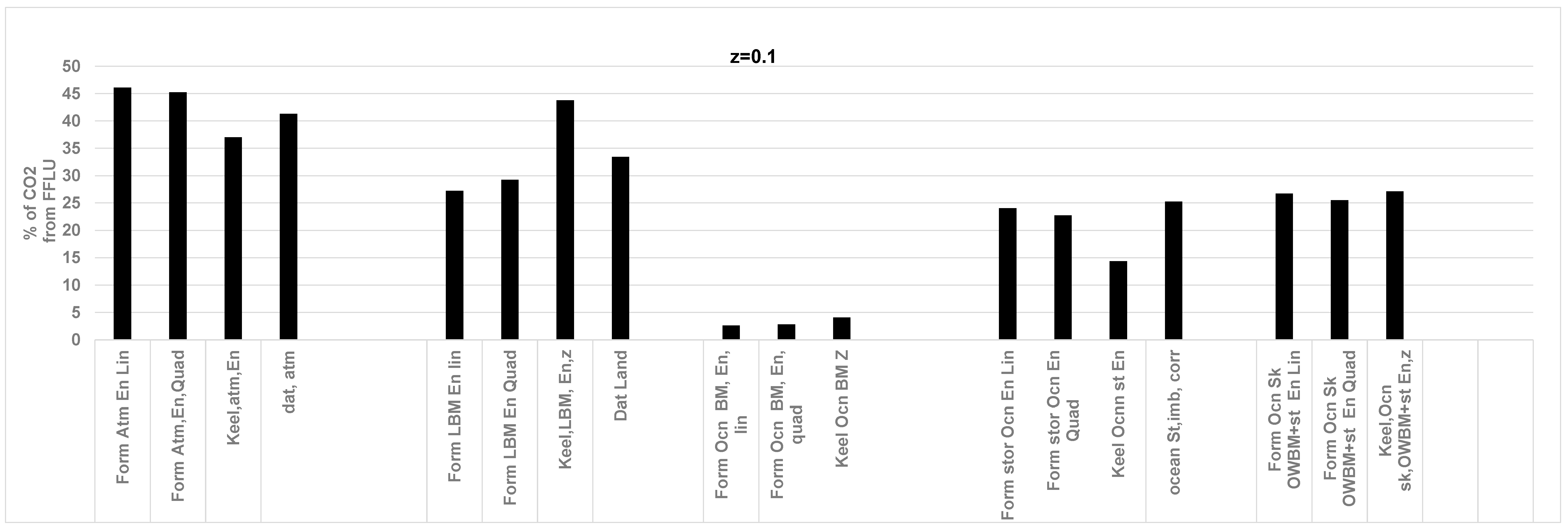
4.4. CO₂ Budget for Year 2006

Readers can skip Section 4.4, which shows the justification for assuming z = 0.1 in presenting the CO₂ budget for 2006, and move on to Section 4.5 for comparisons between the annual results for the CO₂ budget with results from rigorous models with prescribed z. The CO₂ balance via the RQ method yields solutions for CO₂ stored in the atmosphere, CO₂ sink due to LBM and OWBM, and CO₂ stored in the oceans. The relations presented in Table 2 provide the CO₂ distribution through data input from Keeling’s data on CO₂ and O₂ in the atmosphere and annual energy consumption. Only the CO₂ sink data by ocean biomass are not reported, while the current results estimate the total CO₂ sink due to both biomasses (LBM and OWBM). The CO₂ sink by LBM requires a knowledge of a split in O₂ added to the atmosphere by LBM and OWBM or a knowledge of the “z” fraction of O₂ produced by ocean biomass. A step-by-step procedure for the CO₂ budget using the RQ method is indicated in the supplement titled “Supp CO₂ budget Supp Step by Step CO₂ budget”.

4.4.1. O₂ Production by Land and Controversy on O₂ Transfer from Ocean to Atmosphere and z Factor

Ref. [65] suggests that upper ocean water is a source of oxygen. Further, there is a periodic outflow of O₂ in the atmosphere during warm SS (equivalent to 4.5–5.6 GT of C or 12–14.9 GT of O₂) and an inflow from the atmosphere to the ocean in FW [66] But controversy exists about whether the ocean serves as a net oxygen producer or consumer when performing global C and oxygen balance.

Refs. [65,67] suggest that about 50% of oxygen accumulated on Earth originates from ocean PP through photosynthesis in upper 6% of ocean volume. The UN website [68] indicates that 50% of photosynthesis occurs on land, the other 50% in the oceans, and 25% of C is absorbed by the oceans. Others cite that the O₂ produced is about 50–70% of the total O₂ generated [69]. This statement refers only to oxygen currently in the atmosphere, i.e., O₂ stocks (=0.21 * 1.77 × 10⁵ = 37,000 Peta moles of O₂), 50% of which originated from biomass in the oceans (i.e., 18,500 Peta moles). The ocean storage is about 220 Peta moles (0.6% of atmospheric O₂) of dissolved oxygen. Thus, at first glance, z ≈ 0.5 based on UN data, but this does not mean that all of the O₂ produced by OWBM is delivered to the atmosphere or that 50–70% of the air humans currently breathe in comes from the oceans. Skeptics argue [23] that the PP near the ocean surface (data at 20 m and 100 m in Ref. [24]) consumse CO₂ and produce O₂, but MOM (which includes marine microbes and animals) consumes all of this oxygen, apart from dissolved oxygen, and produces CO₂. See also Ref. [70]. So, PP serves as a renewable nutrient or “fuel” for marine life; hence, there is no net O₂ delivered to the atmosphere or net CO₂ sink due to OWBM. However, the ocean is saturated with O₂ near the surface due to a high O₂ concentration in the atmosphere (21% O₂ or 210,000 ppm; it is much higher than CO₂, which is only about 400 ppm). Then, if PP produces O₂, it must supersaturate the O₂ near the surface, and if so, the extra O₂ produced by PP near the ocean surface may enter either the atmosphere or be circulated to deeper parts of the ocean. The global oxygen balance studies by Huang et al. [25] state that only 1.74 GT/year of oxygen enters the atmosphere from the ocean, while land-based biomass generates 16.01 GT/year, indicating about 10% of total O₂ from OWBM. See Appendix C, which presents another method of estimating z from the knowledge of C sink via land biomass. For the present study, z is treated as a parameter varying from 0 to 0.5 for comparing the CO₂ budget based on the RQ method with results from the literature data generated from more detailed models for 2006 and then selecting an appropriate value for “z”.

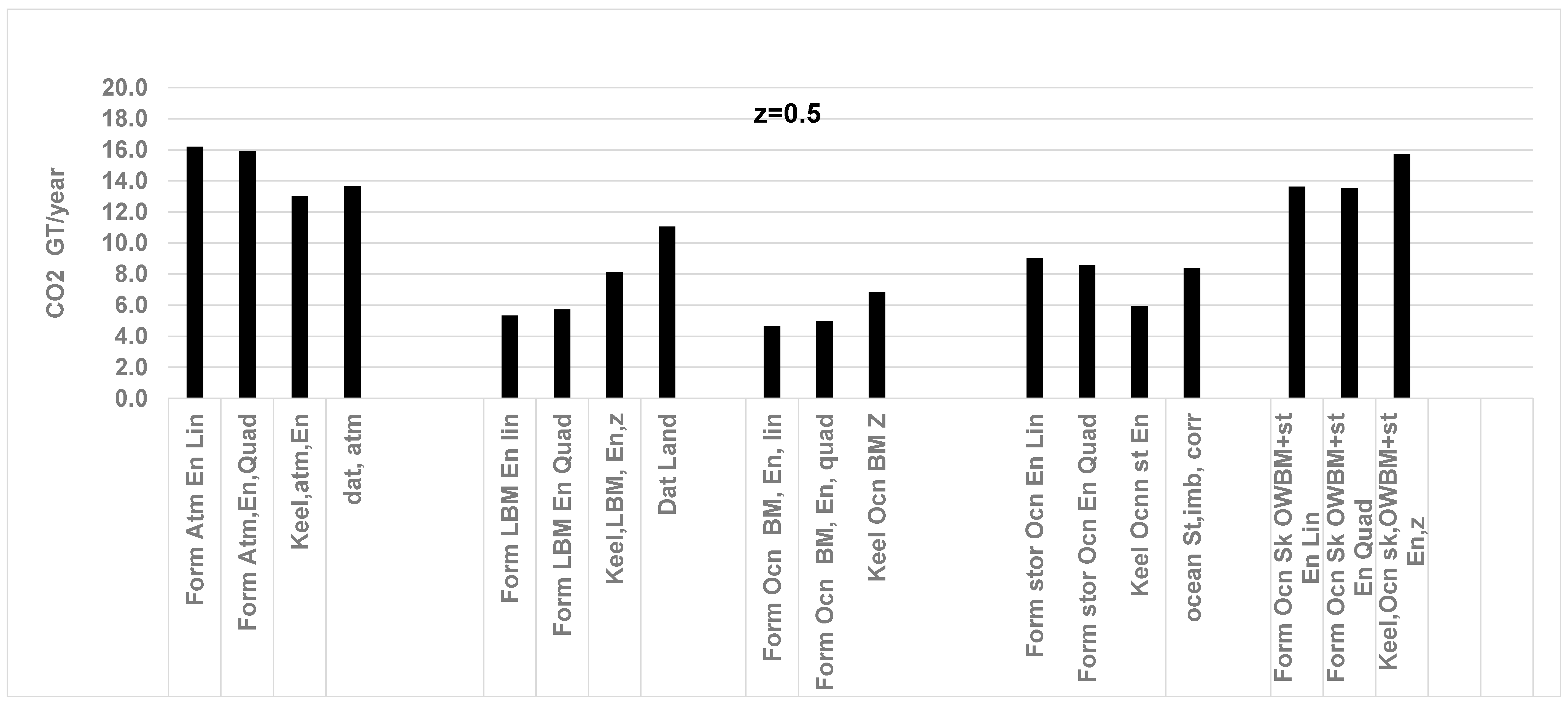
4.4.2. Effects of z on CO₂ Sink by LBM, OWBM, and Ocean Storage

It is shown that the RQ of the combined RQ for land and ocean biomasses (RQ_LOWBM) is affected by the value of “z” (Equation (14)) and, hence, depends on the energy (or O₂) fraction {z} contributed by ocean-type biomass (Equations (14) and (15)) and (1 − z) contributed by LBM. For the year 2006, the results for CO₂ distributions in GT/year and as a % of CO₂ emitted from the atmosphere, land, and ocean are shown in Figure 4 and Figure 5 for z = 0, Figure 6 and Figure 7 for z = 0.1, and Figure 8 and Figure 9 for z = 0.5.

Results in these figures are shown for the following methods: (i) Linear fit of Keeling’s data {Form.Lin} and (ii) Quadratic fits {Form.Quad} with constants summarized in data Section 3.4.2. Both of these results fall under the formula {Form} method; (iii) Keeling’s data {Keel.atm} as it is for the year 2005–2006 (no curve fits, year-to-year basis), (iv) the literature data {Dat.atm} on % and GT/year for the atmosphere, land biomass, and ocean sink/storage. The method from (iii) is based on 2005–2006 data only and is subject to more errors due to fluctuating data from year to year. Most discussions are based on curve fit constants from the quadratic method and comparison with reported data. The last two lines in the figure captions give computed GT/year (quadratic method), while previous data are presented in parentheses.

The results from Figure 4, Figure 5, Figure 6, Figure 7, Figure 8 and Figure 9 can be summarized as follows:

• The results for CO₂ sink in the atmosphere are not affected by z.
• The ocean CO₂ storage is close to the reported data literature for all z (z = 0, 0.1, 0.5) and is a weak function of “z”. The reasons are as follows: the O₂ production by biomass is the difference between O₂ consumption by FFLU and actual O₂ removed from the atmosphere. Thus, once O₂ production is determined, the RQ_LOWBM of combined biomass from the land and ocean determines the amount of CO₂ sink, which is O₂ production * RQ_LOWBM. The RQ_LOWBM of combined biomasses is a weak function of z. The CO₂ balance dictates that the CO₂ storage (= CO₂ produced by FFLU − CO₂ sinks via combined land and ocean biomass) is a weak function of z.
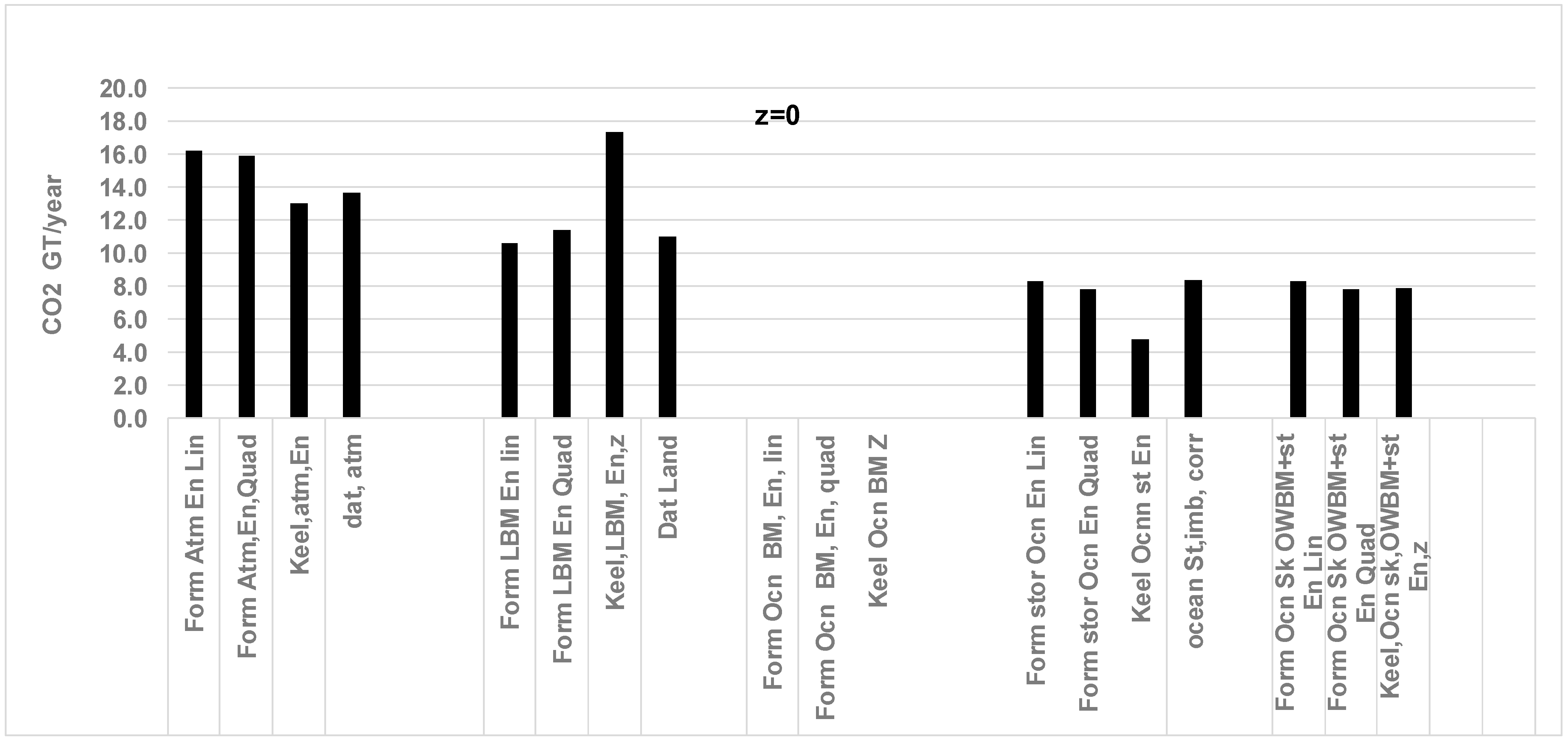
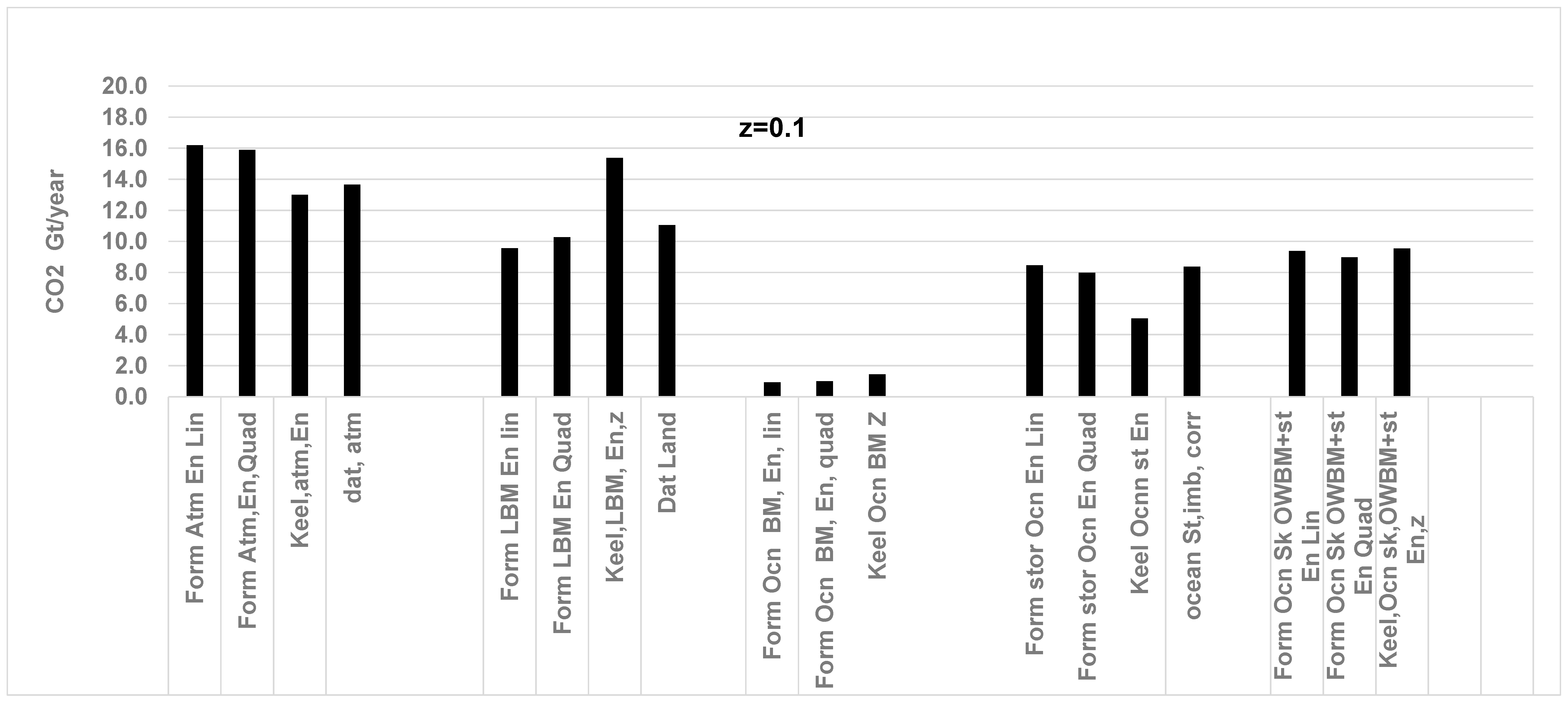
• There is a budget imbalance % in the previous literature data on C or CO₂, which is given as [(FFLU CO₂ source − CO₂ added to the atmosphere − CO₂ used by both land and ocean biomasses − CO₂ stored by ocean water) * 100/ FFLU CO₂ source]. The imbalance is about 7% [50]. For example, the CO₂ added to the atmosphere is 15.9 GT/year, while data provided by the “stand-alone” atmosphere models indicate only 13.7 GT/year. However, the current formulation with the RQ method is based on the CO₂ or C balance method, i.e., the literature data reported on CO₂ must be increased by 7%, or data for atmosphere must be increased to 14.7 GT/year when compared with results from the RQ model.
• All the numbers were cross-checked by starting from the end results and back-calculating Keeling’s data (ppm of CO₂ added to the atmosphere and ppm O₂ removed from the atmosphere) for the following cases. (i) First estimate the ppm of CO₂ added to the atmosphere and O₂ removed from the atmosphere due to FFLU alone, in case there was no biomass or ocean storage in 2006; (ii) Then, estimate the ppm of CO₂ removed and O₂ produced by land and ocean biomasses (based on results for CO₂% removed by land and ocean biomasses) and re-calculate the ppm of CO₂ added to the atmosphere and O₂ depleted from the atmosphere. (iii) Finally, estimate the ppm of CO₂ removed due to storage by ocean water (based on % CO₂ stored by ocean water) and calculate the CO₂ added to the atmosphere. (iv) Verify these numbers (ppm/year) to be the same as Keeling’s data on CO₂ and O₂.
• Using the formula listed Table 2, the CO₂ fractions in the atmosphere, land and ocean BM, and ocean storage {Rows 11, 12 and 13} and the CO₂ loading in GT/year are estimated {Rows 3b,17 and 20}. The sum of the CO₂ fraction in the atmosphere, land and ocean BM, and ocean storage was confirmed to be in unity.
• The RQ method with a quadratic fit for land CO₂ sink is estimated as 10.3 GT/year at z = 0.1, while the reported data are 11.1 GT/year. The results from the RQ method agree closely with the literature data on CO₂ sink by LBM at low values of z (0 < z < 0.1).
• Since RQ_OWBM = 0.87, RQ_LBM = 1, then for z = 0.1, RQ_LOWBM = 0.987 ≈ RQ_LBM (since 90% O₂ added to atm is assumed to come from LBM).
• When z = 0.5 (50% O₂ by ocean biomass or 50% CO₂ by land biomass), the RQ method underpredicts the CO₂ sink by land biomass since the % of O₂ production by land biomass is reduced with a corresponding reduction in CO₂ sink at a fixed RQ_LBM.
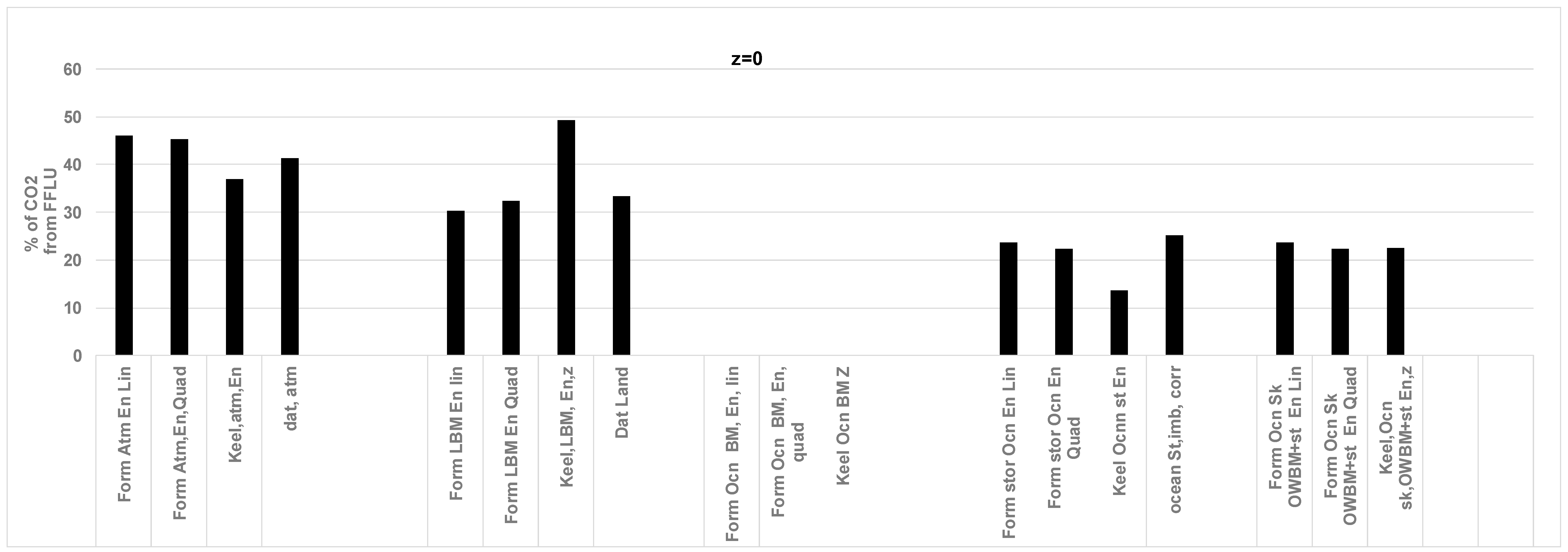
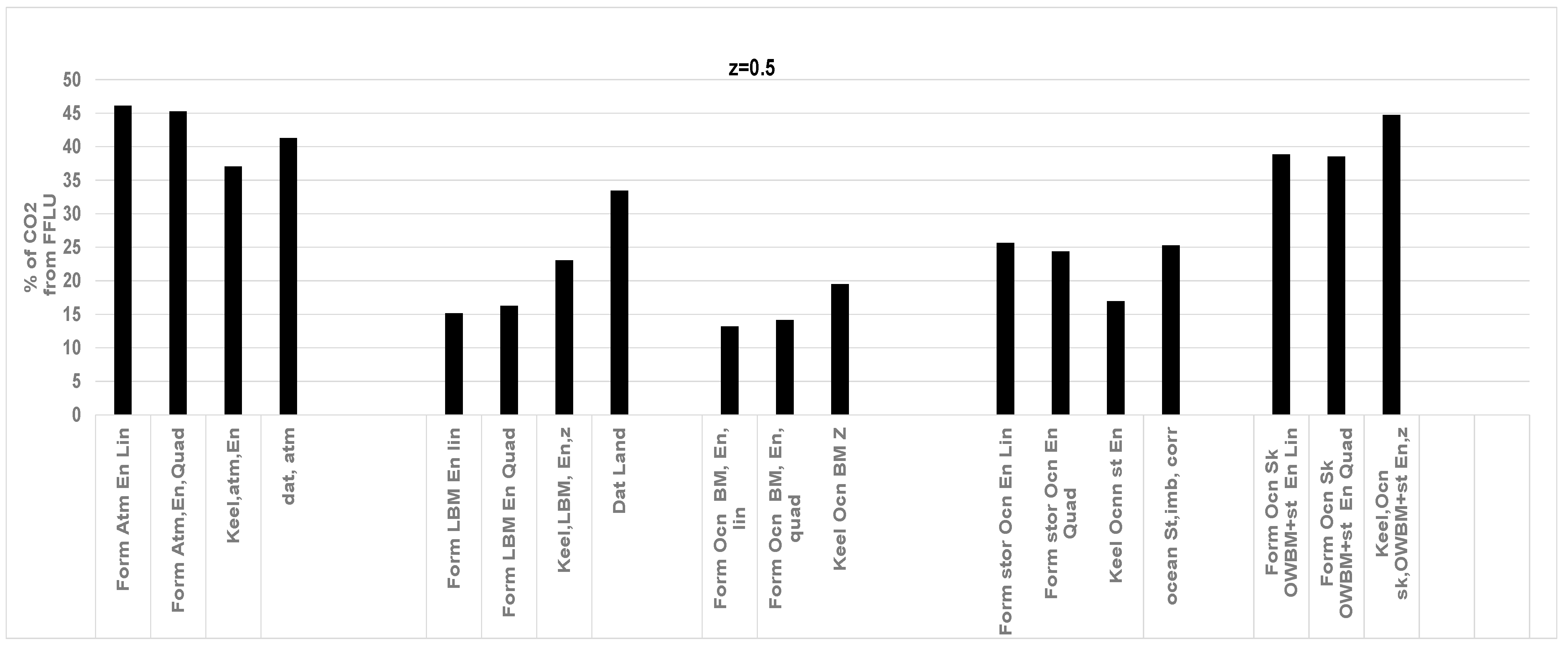
• When the explicit formula (Equation (14) to Equation (16)) was used for the year 2006 with z = 0.1, CO₂ atmosphere % =45.2 (literature: 41.3), CO₂ land BM % = 29.04 (29.2), and (Ocn st + Ocn BM), % = 25.7 (25.3).

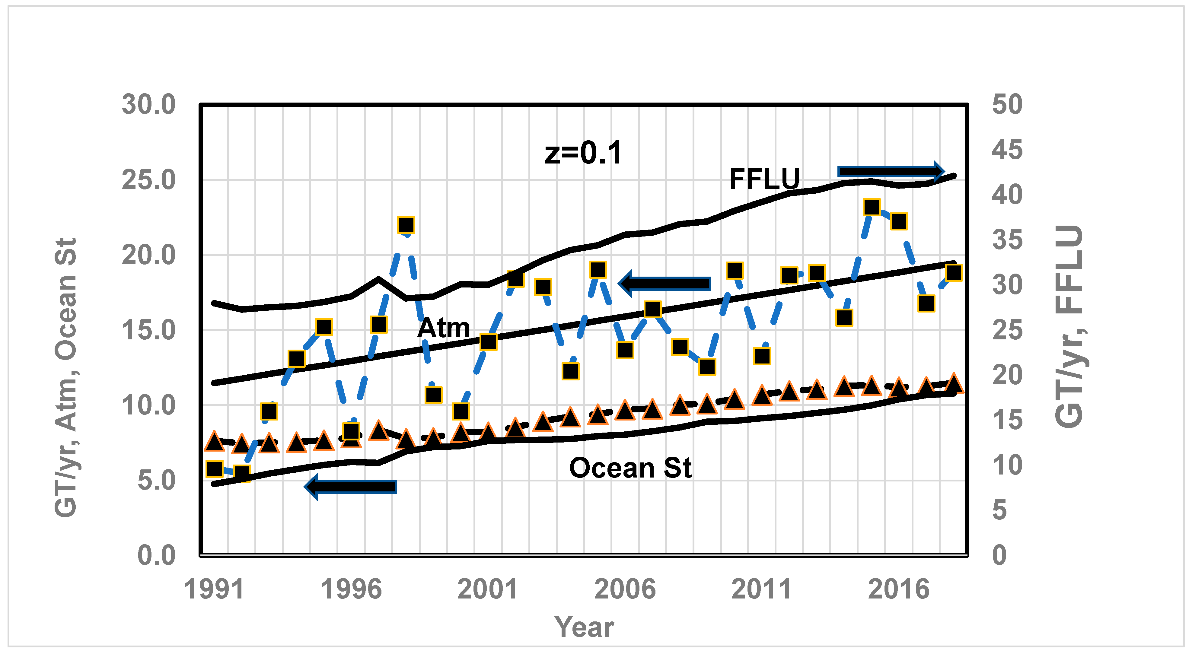
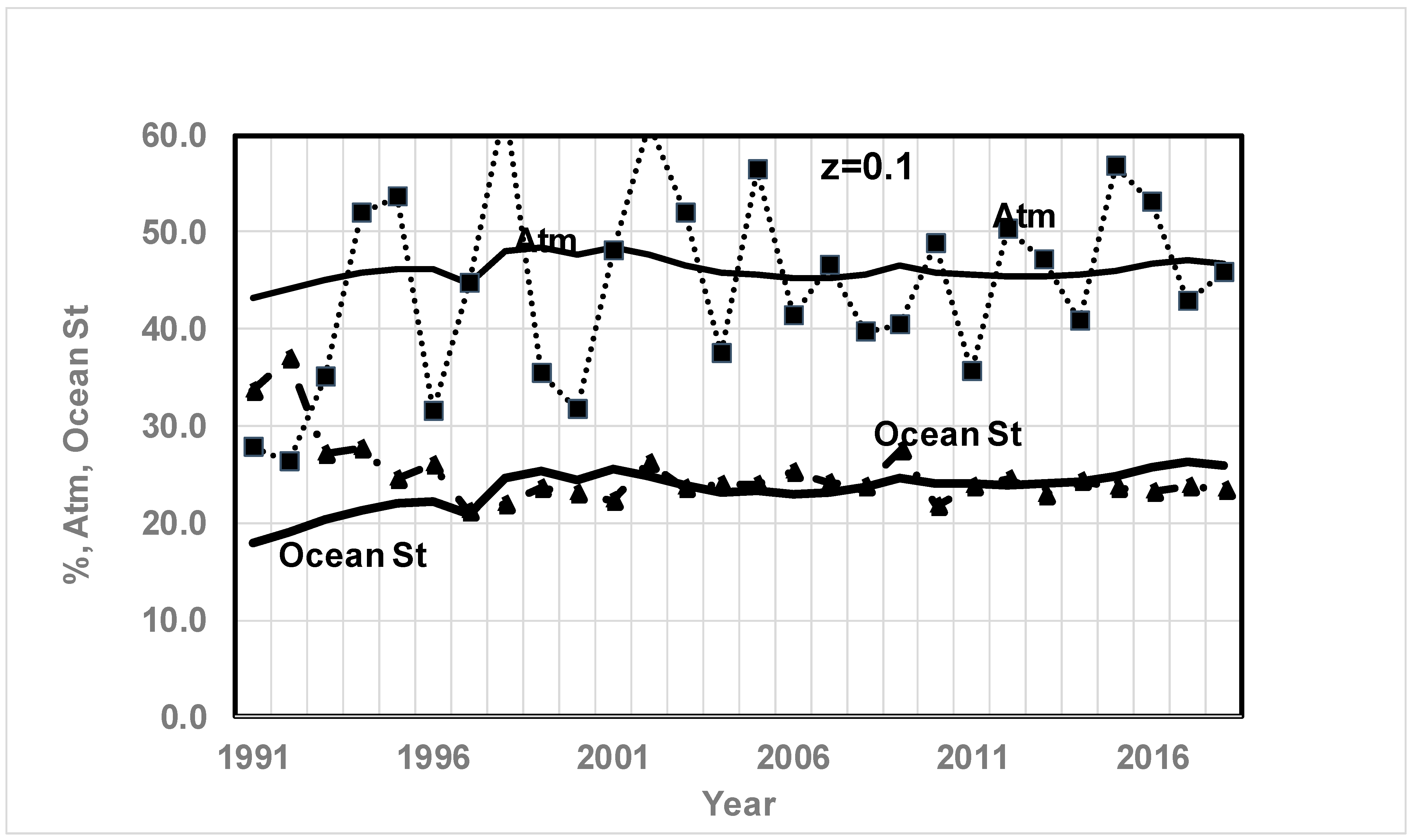
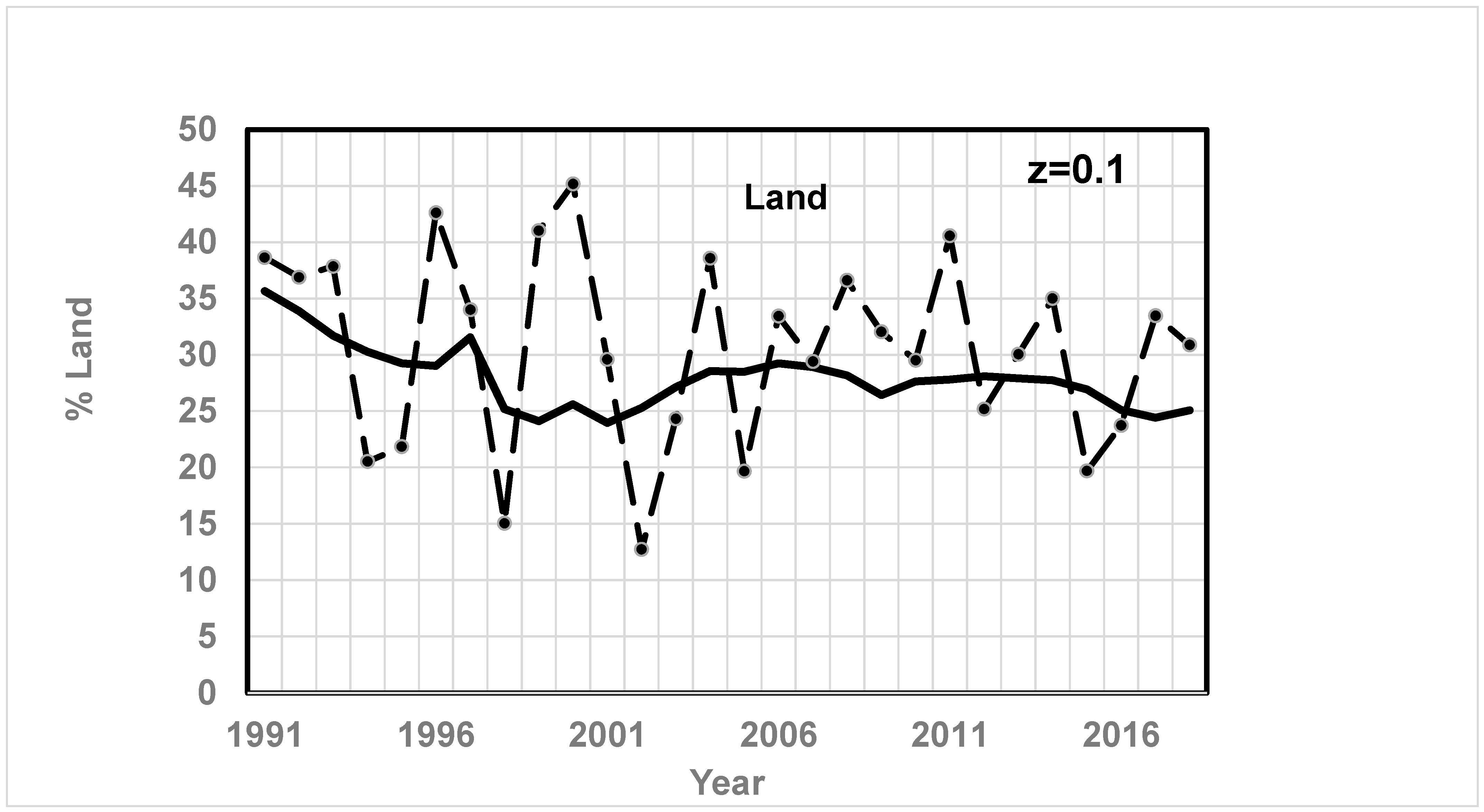
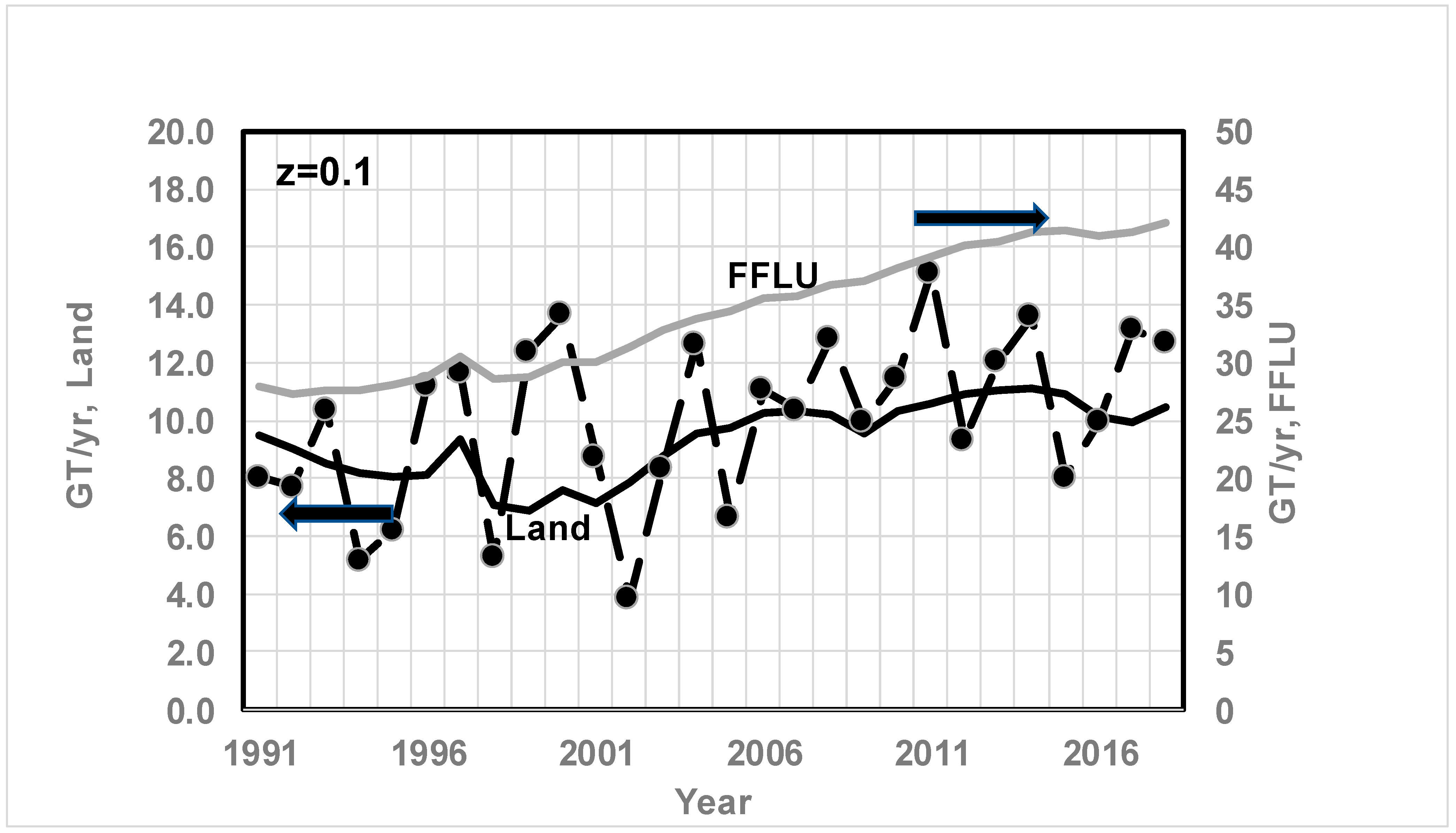
4.5. Comparison of Annual CO₂ from RQ Method with the Reported Annual Data (1991–2020)

The results for CO₂ storage in the atmosphere and ocean are very weak functions of z. Section 4.2 showed that the results on CO₂ sink via LBM were a strong function of z and when z = 0.1, the computed results agreed closely with reported data for the year 2006. In this section, RQ-based results for CO₂ sink via land, atmosphere, and ocean storage {solid lines Figure 10 (GT/year) and Figure 11 (%)} are compared with previously reported data {dashed line with marker} for atmosphere, land, and ocean storage, assuming z = 0.1. The agreement is very close. The data for the atmosphere fluctuates around the smooth curve due to year-to-year variations in wind conditions, temperature, and gradients of CO₂ between land and the atmosphere and ocean and the atmosphere. The predicted results reveal a smooth curve since the prediction is based on curve fit constants. Figure 12 (GT/year) and Figure 13 (%) show a comparison of computed CO₂ sink (solid line) by land biomass with previous data (dashed line with marker). The average C sinks from land and ocean sinks from 2000 to 2016 reported in [28] are 9.53 ±2.57 and 5.59 ± 3.30 GT of CO₂/year (or 2.6 ± 0.7 and 1.5 ± 0.9 GT of C per year), while the RQ method shows CO₂ sink via ocean storage to be 5 to 10 GT /year with an average of 7.5 GT /year and land biomass to be 10.5 GT/year from 1991 to 2018. They are within the error bounds of Tohjima et al.’s work [28]. Ref. [28] also states that their sink estimates are within 1.47 GT/year, as presented by the GCP.

4.5.1. Freezing CO₂ Growth in Atmosphere Using RQ

One can estimate the desired RQ_FFLU so that CO₂ in the atmosphere remains flat or d(CO₂)/dt = 0 in Equation (9). See Appendix B for details.

$$R{Q}_{FFLU}-R{Q}_{LOWBM}\ast x-y==\frac{\left\{\frac{d(CO2)}{dt}\right\}\left(\frac{ppm}{year}\right)\ast F_{Bal}}{{\dot{E}}_{FFLU}}=0.$$

(25)

Required RQ_FFLU: Solving for RQ_FFLU from the above equation,

$$R{Q}_{FFLU}=R{Q}_{LOWBM}x+y$$

(26)

where x is given by Row 7a, Table 2 in terms of annual energy release rate from FFLU, and Row 7b, Table 2 in terms of annual carbon release rate from FFLU and [d(O₂)/dt]_atm.

It is noted that “y” remains almost flat (Figure 3), indicating increased CO₂ storage (hence, ocean acidity) in proportion to O₂ consumption rate by FFLU or annual energy release rate from FFLU. Since CO₂ remains flat, the coefficients d₂, d₁, and d₀ for quadratic fit of O₂ data may be different; hence,

$$\frac{d\left[O_2\right]}{dt}=2\ast e_2+e_1$$

(27)

Figure 3 reveals that variations in x and y are mostly flat (x ≈ 0.3 to 0.2, y ≈ 0.2 to 0.25) compared to FFLU energy, which increases by 60%. Assuming x ≈ 0.25, y = 0.23, RQ_LOWBM = ≈1, the desired RQ_FFLU = 0.48, y = 0.23 (with ocean acidification), and RQ_FFLU = 0.25 (with no ocean acidification, y = 0). The low value of 0.25 for RQ_FFLU is difficult to achieve in practice since the lowest RQ is 0.5 for methane fuel (or natural gas).

Required RQ_LOWBM: If RQ_FFLU is fixed, one may solve for the desired RQ_LOWBM as (Equation (26))

$$R{Q}_{LOWBM}=\left\{\frac{R{Q}_{FFLU}-y}{x}\right\}$$

(28)

If NG is used as a global fossil fuel, the RQ_FFLU = 0.5, and assuming x = 0.25, y = 0.23, the desired RQ_LOWBM = 1.08. Ref. [73] reports an RQ from 1.2 to 2.0 (i.e., PQ as 0.5 to 0.85) for sea weeds. Another avenue for increasing CO₂ sink via biomass is to use AI photosynthesis and photoelectrochemical carbon sinks [74].

4.5.2. Freezing CO₂ Growth in Atmosphere by CO₂ Storage

Carbon Capture and storage: If direct air capture (DAC) technologies are adopted for extracting CO₂ directly from the atmosphere, the required underground storage of CO₂, ${\dot{N}}_{CO2,St,UG}$, is given as

$${\dot{N}}_{CO2,St,UG}={\dot{N}}_{CO2,St,atm}=\left\{\frac{d\left[C{O}_2\right]}{dt}\right\}\left(\frac{ppm}{year}\right)\ast {10}^{-6}\ast N_{air}$$

(29)

where ${\dot{N}}_{CO2,St,UG}$ in Peta moles/year. The required amount of C(s) to be sequestered in mass units is given as

$${\dot{m}}_{C(s),St,UG}={\dot{N}}_{CO2,St,UG}\ast M_C=F_{CGt}\ast {\left\{\frac{d\left[C{O}_2\right]}{dt}\right\}}_{atm}$$

(30)

$${\dot{m}}_{CO2,St,UG}={\dot{m}}_{C(s),St,UG}\frac{M_{CO2}}{M_C}={\dot{m}}_{C(s),St,UG}\ast 3.66$$

where ${\dot{m}}_{C(s),St,UG},{\dot{m}}_{CO2,St,UG}$ are the required amounts to be stored in GT of C(s) and GT of CO₂ per year in the underground (UG) storage for maintaining {d[CO₂]/dt} in the atmosphere = 0. See Row #3b, Table 2.

Several models exist for underground gas storage [75,76]. One can use depleted oil/gas reservoirs as CO₂ underground storage with the additional benefit of reducing Earth’s mass loss rate [9] since CO₂ mass, which would have escaped to the atmosphere, is returned to Earth with underground storage.

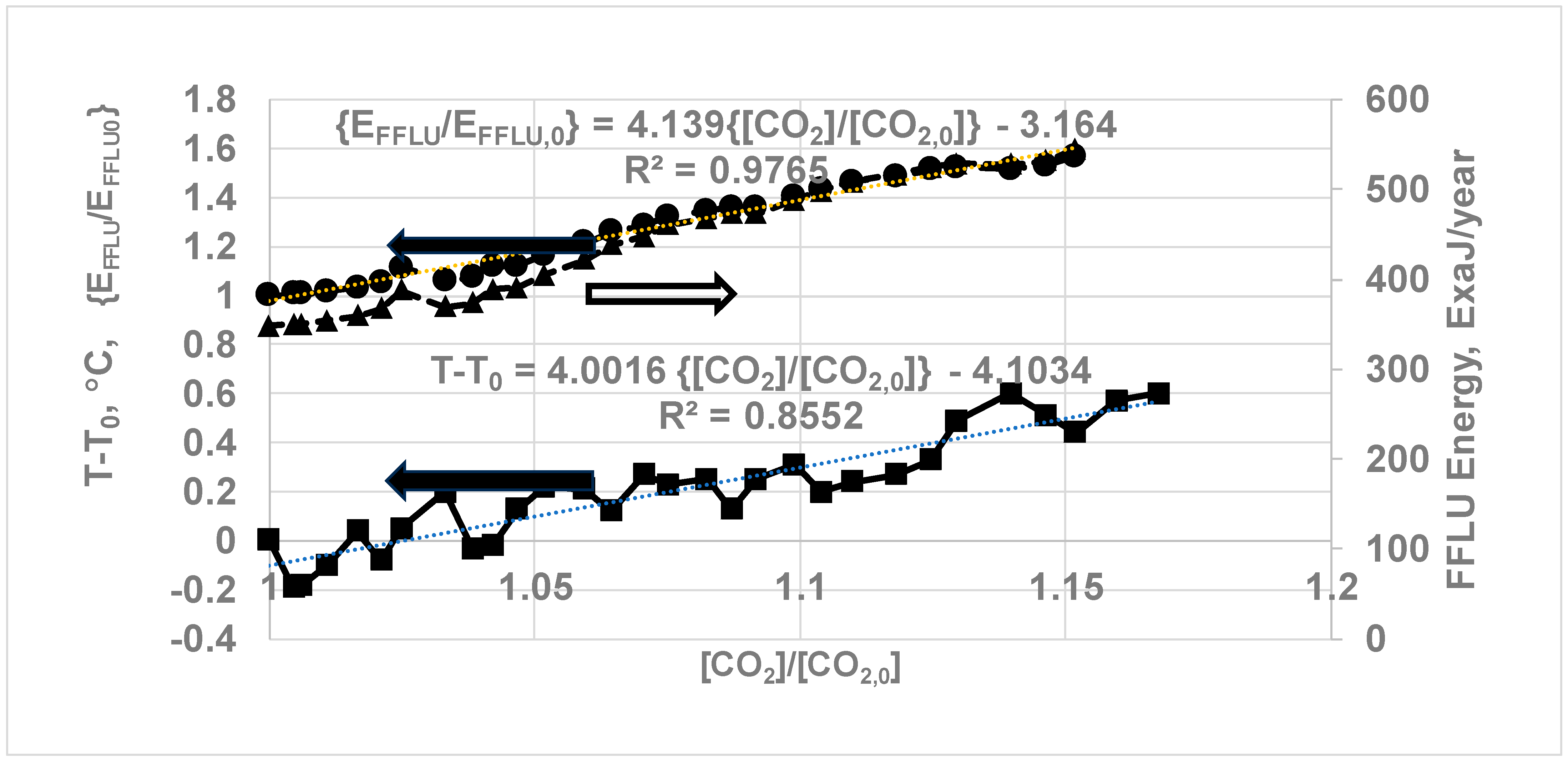
4.6. Relation between Global Temperature, Rate of Heating, Energy, and Global CO₂ Concentration

The authoritative NASA website contains data on land and sea surface temperature (SST) [32]. Most of the data are reported as temperature anomalies, defined as the difference between local temperature and average temperature or base temperature for the specific period of 30 years (1951–1980) at the same location, so the temperature anomaly is location-independent. The global average temperature for 30 years was 13.9 °C or 57 °F [77]. The 2010 global temperature was 14.7 °C, or 0.8 °C was the temperature anomaly in 2010. For additional information, see websites at NASA’s Goddard Institute for Space Studies and NOAA’s National Centers [78].

The quadratic curve fit to the global average temperature since 1880 computed from the temperature anomaly and assuming a global 30-year average (1951–1980) temperature of 13.9 °C (57 F) [79] yields the following relation:

$$T°C=g_2{t}^2+g_{1}t+g_0,R²=0.903,years:1880-2023$$

(31)

where g₂ = 9.114 * 10⁻⁵, g₁ = −5.281 * 10⁻³ t, g₀ = 13.71, t = Year of interest − 1880,

$$\frac{dT}{dt},\left(\frac{°C}{Year}\right) =2 g_2\ast t+g_1$$

(32)

Based on curve fit constants, the heating rate was 0.15 °C/decade (1981–1991), and now it has jumped to 0.22 °C/decade (2012–2022).

Since data are available for both the global average temperature vs. year and Keeling’s data on CO₂ ppm, it is of interest to plot temperature vs. CO₂ concentration, which is related to energy from FFLU. Selecting T₀ for year 1991, the ΔT was then plotted against ([CO₂]/[CO_2,0]) where [CO₂] was the CO₂ concentration in the year of interest and [CO_2,0] was the concentration of CO₂ in the year 1991 (Figure 14). The curve fits for ΔT vs. [CO₂]/ [CO_2,0]) for years 1991–2022 (Figure 14) yields

$$\Delta T ,°C={ \mathrm{h}}_1 \left(\frac{[C{O}_2]}{[C{O}_{2,0}]}\right)+{\mathrm{h}}_0 ,{\mathrm{h}}_1=4.0,{\mathrm{h}}_0=-4.10,[C{O}_{2,0}]=351ppm,R²=0.86$$

(33)

Note that the concentration ratio ([CO₂]/[CO_2,0]) is the same as the GT ratio of CO₂. Differentiating Equation (33), the rate of temperature rise is given as

$$\frac{dT}{dt}=\frac{{\mathrm{h}}_1}{[C{O}_{2,0}]} {\left(\frac{d[C{O}_2]}{dt}\right)}_{atm},{\mathrm{h}}_1=4.0$$

(34)

where {d[CO₂]/dt}_atm in ppm/year and one may use linear or quadratic fit to obtain the slope ${\left(\frac{d[C{O}_2]}{dt}\right)}_{atm}$.

Row #21a, Table 2 for global temperature rise ΔT vs. year.

Row #21b, Table 2 for global temperature rise ΔT vs. [CO₂]/[CO₂]₀.

Row #22a, Table 2 for rate of temperature rise dT/dt in terms of ${\left(\frac{d[C{O}_2]}{dt}\right)}_{atm}$.

Ref. [1] reports 0.0125 °C/year (or 0.125 °C per decade, around 1994) with a CO₂ increase of 2 ppm/year, while Equation (34) with 2.08 ppm/year (Keeling’s data, linear fit) yields 0.023 °C/year or 0.23 °C/decade. The NASA website [77] indicates 0.15–0.20 °C/decade since 1975, while the recent data in 2022 indicates 0.18 °C/decade [80].

In the following, an attempt has been made to relate the rate of heating of Earth to the annual energy release rate {${\dot{E}}_{FFLU}$, Exa J/year}, even though the processes governing the relation are complex (see Ref. [36] for balance equations). Using the definition of RQ_Glob(En), one can express d[CO₂]/dt in the atmosphere as

$${\left(\frac{d\left[CO2\right]}{dt}\right)}_{atm}=F_{CO2}\ast R{Q}_{Glob(En)}\ast {\dot{E}}_{FFLU},F_{CO2}=\left(\frac{{10}^6}{N_{air}\ast HH{V}_{O2}}\right)=0.0126$$

(35)

Figure 3 shows that RQ_Glob(En) is almost constant. Hence, the above equation suggests that the rate of CO₂ increase in the atmosphere (ppm/year) is proportional to ${\dot{E}}_{FFLU}$. Expressing Equation (35) in Equation (34), the rate of heating is given as

$$\frac{dT}{dt}=F_{dTdt}\ast R{Q}_{Glob(En)}\ast {\dot{E}}_{FFLU},F_{dTdt}=\left\{\frac{h_1\ast F_{CO2}}{\left[C{O}_{2,0}\right]}\right\}=1.44\times {10}^{-4}$$

(36)

which shows that the rate of temperature rise is proportional to the energy release rate in Exa J per year.

Row #22b, Table 2 for the rate of temperature rise dT/dt in terms of RQ_Glob(En) and energy release rate.

While the relation for dT/dt with d[CO₂]/dt has a slope of 4 (Equation (34)), Equation (36) indicates the weaker relation of dT/dt with the annual energy release rate. The cumulative energy release from 1991 to 2018 (total of 27 years) via FFLU was about 12,000 Exa J added to Earth (which is almost 40 times more than FFLU energy in 1991), while 4500 GT of CO₂ was added to the atmosphere (which is almost two times the amount present in 1991) during the same period, resulting in the greenhouse effect. Typically, the greenhouse effect is dominant compared to the waste heat/energy release effect.

With 2018 data on ${\dot{E}}_{FFLU}$ = 545 Exa J/year, RQ_Glob(En) = 0.36 from a quadratic fit, Equation (36) yields dT/dt = 0 0.027 °C/year or 0.27 °C/decade. If a linear fit is adopted, RQ_Glob(En) = 0.30, dT/dt = 0.023 °C/year or 0.23 °C/decade. The estimate obtained from the RQ method for Keeling’s curves agrees with the heating rates of 0.28 °C/decade (after 2010) and 0.18 °C per decade (1970–2010) [81], which are based on satellite remote sensing data. The same reference cites similar heating rates by the GCP.

Figure 14 yields the following additional relations:

Figure 14. Variations in global temperature difference (T − T₀) {■}, FFLU energy release rate {▲}, and normalized Energy release $\frac{{\dot{E}}_{FFLU}}{{\dot{E}}_{FFLU,0}}$ {Symbol ●}, with normalized CO₂ concentration, [CO₂]/[CO_2,0] (1991–2020); [CO₂] atmosphere. Arrows ← indicate values on primary axis and → indicate values on secondary axis. Concentration in ppm in any given year and [CO_2,0] atmosphere CO₂ concentration in 1991. Energy and CO₂ data are from Ref. [50]. Global temperature data are from [82]. See data for temperature of NY City in Ref. [83]. The energy release by FFLU (secondary axis), and normalized energy release (primary axis). There are 18% and 60% increases in energy release rate in the years 2006 and 2018, respectively, compared to year 1991.

Figure 14. Variations in global temperature difference (T − T₀) {■}, FFLU energy release rate {▲}, and normalized Energy release $\frac{{\dot{E}}_{FFLU}}{{\dot{E}}_{FFLU,0}}$ {Symbol ●}, with normalized CO₂ concentration, [CO₂]/[CO_2,0] (1991–2020); [CO₂] atmosphere. Arrows ← indicate values on primary axis and → indicate values on secondary axis. Concentration in ppm in any given year and [CO_2,0] atmosphere CO₂ concentration in 1991. Energy and CO₂ data are from Ref. [50]. Global temperature data are from [82]. See data for temperature of NY City in Ref. [83]. The energy release by FFLU (secondary axis), and normalized energy release (primary axis). There are 18% and 60% increases in energy release rate in the years 2006 and 2018, respectively, compared to year 1991.

The normalized energy release rate and hence the normalized CO₂ concentration have the following fits:

$$\begin{array}{l}\frac{{\dot{E}}_{FFLU}}{{\dot{E}}_{FFLU,0}}=i_0+i_1\frac{[CO2]}{[CO2,0]},Or\frac{[CO2]}{[CO2,0]}=\left(j_0+j_1\frac{{\dot{E}}_{FFLU}}{{\dot{E}}_{FFLU,0}}\right),i_0=-3.16,i_1=4.14,j_0=0.76,j_1=0.24\\ R^2=0.98\end{array}$$

(37)

4.7. Limitation of Results

The CO₂ budget results with the RQ method are based on the presumption that Keeling’s data on CO₂ and O₂ in the atmosphere are affected by CO₂ sources from FFLU and CO₂ sinks by biomass and CO₂ storage in the oceans. Thus, if there is an increasing global temperature, it would be reflected in less CO₂ sink by biomass and less O₂ production and vice versa, which are reflected in Keeling’s data. The results do seem to be comparable to the reported literature data, which are based on more detailed fundamental and stand-alone models for the atmosphere, land, and oceans. The results in Table 5 on global O₂ concentration and mass of earth vs. year are based upon the extrapolation of quadratic fit to Keeling’s data as though CO₂ distributions continue the same trends, and they are independent of global temperature and increasing CO₂ concentrations and sea levels.

4.8. Policies and Econometry

Policies: Economic growth measured in terms of a nation’s GDP (gross domestic product) is intricately coupled with the growth of energy consumption. If the source of energy is from the combustion of fossil fuels, the higher the GDP, the higher the energy consumption and the more CO₂. The Intergovernmental Panel on Climate Change (IPCC) recommends climate action via policies limiting global warming to 1.5 °C, which requires a quantum leap in policies to reduce the slope of [CO₂] vs. year. The benefits of CO₂ reduction vs. the cost of policies and the social cost of carbon (SCC), a dollar measure of the “cost” damage to society as a result of CO₂ added to the atmosphere, were investigated by Fraas et al. [84]. The cost of promoting clean technology and net zero emissions must be balanced against the SCC.

The policies require changes in the “upstream” and “downstream” of CO₂ production.

Upstream: (i) Mandates for utilities to adopt low-carbon FFs in electricity generation by a specified deadline, (ii) recommendation on “layered” tax and increased excise taxes, based on the RQ of FFs (a measure of CO₂ emission in tons per unit energy release, e.g., coal with RQ = 1 vs. NG with RQ = 0.5), (iii) use of Ref. [47] in estimating the reduced RQ for a mix of FFs and renewable fuels (RFs) (e.g., gasoline-ethanol blend) and added incentives along with reduced taxes for RFs, and (iv) promotion of solar power.

Downstream: (i) Cap-and-trade regulations, (ii) tax incentives for mitigation, (iii) CO₂ per kWH (which involves efficiency and an increase in cost of electricity generation when meeting mandates) and carbon taxes; e.g., Sweden: USD 30 per ton of CO₂ in 1991 and increased to USD 132 [85], (iv) carbon capture and storage (CCS) and approximate estimation of C to be sequestered using the relations provided in the current text, (v) emissions trading systems with high USD cost of CO₂ per ton, indicating the extent of enforcement of the Paris accord and vice versa, (vi) CO₂ tax based on actual CO₂ emissions rather than transport vehicle weight estimated from the RQ value of fuels [6] and actual fuel consumed, (vii) residential and industrial non-electricity FFs use (e.g., home use for heating and cooking, shops and offices).

Cost: Cost has been identified as the major barrier to implementing CO₂ capture and storage or utilization technologies [86]. Higher adoption of CO₂ capture technologies in various heavy industries will be based on the carbon tax credits and policy framework across different countries [87]. It should be noted that the Internal Revenue Code (IRC) Section 45Q of the US tax code provides tax credits for qualified carbon dioxide captured and sequestered. However, additional policies around the transportation of captured carbon, storage, and taxation of unabated carbon dioxide should be enacted for large-scale implementation of the CO₂ capture technologies and negative or positive outcomes [88,89].

5. Summary

The power plants breathe in O₂ from the atmosphere, oxidize FFs and breathe out CO₂. The RQ_FF varies from 0.5 (NG) to 1.0 (coal). Global RQ is expressed in two forms: (I) RQ_Glob (= CO₂ added to the atmosphere/O₂ depleted from the atmosphere), which is at about 0.47, and (II) RQ_Glob(En) (= CO₂ to the atmosphere/O₂ consumed by FFLU from the atmosphere), which is about 0.36. The definition of RQ_Glob(En) leads to an estimation of CO₂ in GT in the atmosphere per Exa J released by FFLU = 0.1 * RQ_Glob(En). If RQ_Glob or RQ_Glob(En) decreases, this indicates less CO₂ in the atmosphere and higher CO₂ storage and, hence, increased acidity of the oceans. The RQ_Glob(En) of 0.36 implies that 0.36 moles of CO₂ are added to the atmosphere for every mole of O₂ used by FFLU in releasing energy. The CO₂ release by FFLU increased from 27 to 42 GT/year by FFLU for the period 1991–2020.

The simple RQ method of analysis of Keeling’s data leads to explicit formulae for CO₂ sinks in the atm, land and ocean biomasses, and storage in the oceans. The computed results with a quadratic curve fit agree with most of the reported data for CO₂ sink via land biomass (GT per year and %) for the year 2006 when z (the ratio of O₂ contributed by the ocean to the atmosphere/total O₂ contributed by both land and ocean biomasses) is selected to be about 0.1. Computed results for CO₂ storage in the atmosphere and ocean are weak functions of z and agree closely with the collected data.

The RQ concept Is extended for the period of 1991–2020 for estimating the annual CO₂ distribution in GT/year and as a % of CO₂ produced by FFLU by assuming z = 0.1. The RQ-based results are then validated with the literature data (1991–2020) generated using a rigorous model, which includes the effects of wind velocity, temperature, and gradients of CO₂ (i) between land and the atmosphere and (ii) ocean and the atmosphere, and ocean circulation and temperature; thus, the data fluctuate from year to year. However, the predicted results for CO₂ sinks reveal a smooth curve, since the prediction is based on curve fit constants. The RQ method using Keeling’s data shows the variations in CO₂ sink by the atmosphere, land, and ocean as follows: 12 to 33 GT/year (atmosphere), 8 to 10 GT/year (land biomass), and 5 to 10 GT/year as storage in the oceans.

If slow, gradual extinction is a part of the evolution of life on Earth, the planet seems to be marching towards slow extinction due to the time lag between the development of human traits and the fast-changing local climate affected by increasing CO₂ concentration. Just as in biology where nutritional “therapy” is used to control RQ and reduce acidity in the blood, the FFs “therapy” requires low RQ fuels and high RQ biomasses. The sargassum (seaweed) has an RQ of 1.2 to 2.0 [9,73]. The rate of temperature rise with the change in CO₂ concentration is presented, and Keeling’s data seem to suggest a 0.23 °C rise per decade, while NASA’s data indicate a 0.15–0.20 °C rise per decade.

6. Future Work

It was shown that the warming causes an increasing vapor pressure deficit (VPD) {difference between the saturation pressure of H₂O in the atmosphere, P^satH₂O, which increases with temperature, and actual vapor pressure over land and the oceans (p_H2O)} within the globe, creating plant stress, soil drought, and reducing the life span of vegetation [90]. The impact of the VPD on atmospheric pressure, wind velocity, rain, and hurricanes must be studied. Algae (chemical formula: (CH₂O)₁₀₆(NH₃)₁₆(H₃PO₄) or C₁₀₆H₂₆₃N₁₆O₁₀P including PP) can serve as a renewable fuel and can minimize the use of FFs for energy.

It is noted that the control of pollutant emissions sometimes results in global warming in addition to CO₂. The white reflective clouds formed when SO₂, a pollutant, is mixed with water vapor reflect solar energy away from Earth, resulting in more global warming [1]. Thus, future work requires the effects of pollution control on global warming.

There is uncertainty in the literature on the % of O₂ contributions by the ocean to the atmosphere and more precise data are required. Data on the relation between the RQ of biomasses and their variation with the increasing concentration of CO₂ are required. High RQ values for biomass are desired to provide more CO₂ sink by land and ocean biomass. But low RQ values are desired by the same biomasses to provide more O₂ production if O₂ concentrations need to remain at current level! The ideal scenario is to have a “phytoplankton forest” in the ocean along with seaweed. Botanists must explore the possibility of genetically modifying biomasses (e.g., PP in ocean and plants and trees on the land) and using artificial photosynthesis mimicking the natural photosynthesis for serving as a CO₂ sink and O₂ source to provide a high RQ and overcome the economic hurdles [91]. The effects of earth’s mass loss due to mining of FF on earth’s tilt angle must be investigated.

Are Keeling’s data an ultimate judgement of what is happening with CO₂ sources and sinks, land and ocean biomasses, and ocean storage? Is Earth marching towards “death” without any respiration on the planet? Though it is suggested that the Earth has a life period of another 1700 years, extrapolating Keeling’s data, more detailed modeling is required to predict the decreasing oxygen concentration in the atm and the slow extinction of species on Earth.

References

1. Duursma, E.K.; Boisson, M.P. Global Oceanic and Atmospheric Oxygen. Oceanol. Acta 1994, 17, 117–141. [Google Scholar]
2. Schmiege, S.C.; Heskel, M.; Fan, Y.; Way, D.A. It’s only natural: Plant respiration in unmanaged systems. Plant Physiol. 2023, 192, 710–727. [Google Scholar] [CrossRef]
3. Pries, H.C.P.; Angert, A.; Castanha, C.; Hilman, B.; Torn, M.S. Using respiration quotients to track changing sources of soil respiration seasonally and with experimental warming. J. Biogeoscience 2020, 17, 3045–3055. Available online: https://bg.copernicus.org/articles (accessed on 28 January 2024). [CrossRef]
4. Feely, R.A.; Sabine, C.L.; Takahashi, T.; Wanninkhof, R. Uptake and Storage of Carbon Dioxide in the Ocean: The Global CO2 Survey. JGOFS Oceanogr. 2001, 14, 18–32. [Google Scholar] [CrossRef]
5. Gruber, N.; Gloor, M.; Fan, S.-M.; Sarmiento, J.L. Air-sea flux of oxygen estimated from bulk data: Implications for the marine and atmospheric oxygen cycles. Glob. Biogeochem. Cycles 2001, 15, 783–803. [Google Scholar] [CrossRef]
6. Mehmood, T.; Hassan, M.A.; Li, X.; Ashraf, A.; Rehman, S.; Bilal, M.; Obodo, R.M.; Mustafa, B.; Shaz, M.; Bibi, S.; et al. Mechanism behind Sources and Sinks of Major Anthropogenic Greenhouse Gases, Climate Change Alleviation for Sustainable Progression; CRC Press: Boca Raton, FL, USA, 2022; Chapter 8; ISBN 9781003106982. [Google Scholar]
7. U.S. EPA. 2020 Common Reporting Format (CRF); U.S. EPA Environmental Protection Agency: Washington, DC, USA, 2020.
8. Gasser, T.; Crepin, L.; Quilcaille, Y.; Houghton, R.A.; Ciais, P.; Obersteiner, M. Historical CO2 emissions from land use and land cover change and their uncertainty. Biogeosciences 2020, 17, 4075–4101. [Google Scholar] [CrossRef]
9. Annamalai, K. Breathing Planet Earth: Global Respiratory Quotient (RQGlob) from Keeling’s Data and CO2-Budget among the Atmosphere, Land and Oceans, Part I: Brief Review on RQ and Global Respiratory Quotient of Earth. J. Energy 2023, 17, 299. [Google Scholar]
10. Available online: https://www.theguardian.com/commentisfree/2008/aug/13/carbonemissions.climatechange (accessed on 1 January 2024).
11. Martin, D.; McKenna, H.; Livina, V. The human physiological impact of global deoxygenation. J. Physiol. Sci. 2017, 67, 97–106. [Google Scholar] [CrossRef]
12. Livina, V.N.; Martins, T.M.; Forbes, A.B. Tipping point analysis of atmospheric oxygen concentration. Chaos 2015, 25, 036403. [Google Scholar] [CrossRef]
13. Available online: https://news.climate.columbia.edu/2022/01/27/how-climate-change-will-affect-plants/ (accessed on 7 December 2023).
14. Available online: https://en.wikipedia.org/wiki/Composition_of_the_human_body (accessed on 25 August 2023).
15. Available online: https://ourworldindata.org/life-by-environment (accessed on 14 January 2023).
16. Gruber, N.; Clement, D.; Carter, B.R.; Feely, R.A.; van Heuven, S.; Hoppema, M.; Ishii, M.; Key, R.M.; Kozyr, A.; Lauvset, S.K.; et al. The oceanic sink for anthropogenic CO2 from 1994 to 2007. Science 2019, 363, 1193–1199. [Google Scholar] [CrossRef]
17. Falkowski, P.G. The role of phytoplankton photosynthesis in global biogeochemical cycles. Photosynth. Res. 1994, 39, 235–258. [Google Scholar] [CrossRef]
18. Available online: https://socratic.org/questions/55c2531d581e2a136c45b148 (accessed on 28 January 2024).
19. Behrenfeld, M.J. Climate-mediated dance of the plankton. Nat. Clim. Chang. 2014, 4, 880–887. [Google Scholar] [CrossRef]
20. Available online: https://mynasadata.larc.nasa.gov/basic-page/global-phytoplankton-distribution (accessed on 15 April 2023).
21. Available online: https://ugc.berkeley.edu/background-content/oxygen-levels/ (accessed on 15 January 2024).
22. Zhao, R.; Zhang, I.H.; Jayakumar, A.; Ward, B.B.; Babbin, A.R. Origin, age, and metabolisms of dominant anammox bacteria in the global oxygen deficient zones. bioRxiv 2023. [Google Scholar] [CrossRef]
23. Available online: https://theconversation.com/humans-will-always-have-oxygen-to-breathe-but-we-cant-say-the-same-for-ocean-life-165148 (accessed on 6 February 2023).
24. Balkanski, Y.; Monfray, P.; Battle, M.; Heimann, M. Ocean primary production derived from satellite data: An evaluation with atmospheric oxygen measurements. Glob. Biogeochem. Cycles 1999, 13, 257–271. [Google Scholar] [CrossRef]
25. Huang, J.; Huang, J.; Liu, X.; Li, C.; Ding, L.; Yu, H. The global oxygen budget and its future projection. Sci. Bull. 2018, 63, 1180–1186. [Google Scholar] [CrossRef]
26. Long, M.C.; Ito, T.; Deutsch, C. Oxygen projections for the future. In Ocean Deoxygenation: Everyone’s Problem—Causes, Impacts, Consequences and Solutions; Laffoley, D., Baxter, J.M., Eds.; IUCN: Gland, Switzerland, 2019; Chapter 4; pp. 171–211, xxii+56. [Google Scholar]
27. Keeling, R.F.; Manning, A.C. Studies of Recent Changes in Studies of Recent Changes in Atmospheric O2 Content. In Treatise on Geochemistry, 2nd ed.; Holland, H.D., Turekian, K.K., Eds.; Elsevier: Amsterdam, The Netherlands, 2014; pp. 385–404. [Google Scholar] [CrossRef]
28. Tohjima, Y.; Mukai, H.; Machida, T.; Hoshina, Y.; Nakaoka, S. Global carbon budgets estimated from atmospheric O2/N2 and CO2 observations in the western Pacific region over a 15-year period. Atmos. Chem. Phys. 2019, 19, 9269–9285. [Google Scholar] [CrossRef]
29. Webb, P. Introduction to Oceanography; Chapter 5, Digital Book; Rebus Community: Montreal, Quebec, Canada. Available online: https://rwu.pressbooks.pub/webboceanography (accessed on 28 January 2024).
30. Available online: https://newportbay.org/ask-a-naturalist-do-phytoplankton-produce-more-oxygen-than-a-rainforest-if-so-does-the-oxygen-they-produce-go-into-the-atmosphere-or-does-it-just-remain-dissolved-in-the-ocean/ (accessed on 26 February 2023).
31. Lenssen, N.; Schmidt, G.; Hansen, J.; Menne, M.; Persin, A.; Ruedy, R.; Zyss, D. Improvements in the GISTEMP uncertainty model. J. Geophys. Res. Atmos. 2018, 124, 6307–6326. [Google Scholar] [CrossRef]
32. Available online: https://climatedataguide.ucar.edu/climate-data/global-temperature-data-sets-overview-comparison-table (accessed on 31 July 2023).
33. Hansen, J.; Ruedy, R.; Sato, M.; Lo, K. Global surface temperature change. Rev. Geophys. 2010, 48, RG4004. [Google Scholar] [CrossRef]
34. NOAA; National Centers for Environmental Information. State of the Climate: Global Climate Report for 2022. 2023. Available online: https://www.ncei.noaa.gov/access/monitoring/monthly-report/global/202213 (accessed on 28 January 2024).
35. Available online: https://www.climate.gov/news-features/understanding-climate/international-report-2021-climate-record-high-greenhouse-gases (accessed on 12 September 2023).
36. Chaisson, E.J. Long-Term Global Heating from Energy Usage. Eos Trans. AGU 2008, 89, 253–254. [Google Scholar] [CrossRef]
37. Schuckmann, K.; Minère, A.; Gues, F.; Cuesta-Valero, F.J.; Kirchengast, G.; Adusumilli, S.; Straneo, F.; Ablain, M.; Allan, R.P.; Barker, P.M.; et al. Heat stored in the Earth system 1960–2020: Where does the energy go? J. Earth Syst. Sci. Data 2023, 15, 1675–1709. [Google Scholar] [CrossRef]
38. Available online: https://www.ncei.noaa.gov/access/monitoring/monthly-report/global/202303 (accessed on 7 June 2023).
39. Available online: https://www.un.org/development/desa/jpo/wp-content/uploads/sites/55/2017/02/2030-Agenda-for-Sustainable-Development-KCSD-Primer-new.pdf (accessed on 15 February 2024).
40. Available online: https://www.ipcc.ch/sr15/ (accessed on 1 February 2024).
41. Kim, S.K.; Shin, J.; An, S.I.; Kim, H.J.; Im, N.; Xie, S.P.; Kug, J.S.; Yeh, S.W. Widespread irreversible changes in surface temperature and precipitation in response to CO2 forcing. Nat. Clim. Chang. 2022, 12, 834–840. [Google Scholar] [CrossRef]
42. Duffy, K.A.; Schwalm, C.R.; Arcus, V.L.; Koch, G.W.; Liang, L.L.; Schipper, L.A. How close are we to the temperature tipping point of the terrestrial biosphere? Sci. Adv. 2021, 7, eaay1052. [Google Scholar] [CrossRef]
43. Available online: https://climate.mit.edu/ask-mit/how-will-future-warming-and-co2-emissions-affect-oxygen-concentrations (accessed on 15 January 2024).
44. Friedlingstein, P.; O’sullivan, M.; Jones, M.W.; Andrew, R.M.; Gregor, L.; Hauck, J.; Quéré, C.L.; Luijkx, I.T.; Olsen, A.; Peters, G.P.; et al. Global Carbon Budget 2022. Earth Syst. Sci. Data 2022, 14, 4811–4900. [Google Scholar] [CrossRef]
45. Thanapal, S.S.; Annamalai, K.; Lawrence, B.; Sweeten, J.M. Biomass Co-Combustion with Coal. In Reference Module in Earth Systems and Environmental Sciences; Elsevier: Amsterdam, The Netherlands, 2023; ISBN 9780124095489. [Google Scholar] [CrossRef]
46. Keeling, C.D.; Piper, S.C.; Bacastow, R.B.; Wahlen, M.; Whorf, T.P.; Heimann, M.; Meijer, H.A. Atmospheric CO2 and 13CO2 Exchange with the Terrestrial Biosphere and Oceans from 1978 to 2000: Observations and Carbon Cycle Implications. In A History of Atmospheric CO2 and Its Effects on Plants, Animals, and Ecosystems; Ecological Studies; Springer: New York, NY, USA, 2005; Volume 177, pp. 83–113. [Google Scholar] [CrossRef]
47. Annamalai, K.; Thanapal, S.; Ranjan, D. Ranking renewable and fossil fuels on global warming potential using respiratory quotient (RQ) Concept. J. Combust. 2018, 2018, 1270708. [Google Scholar] [CrossRef]
48. Schmidtko, S.; Stramma, L.; Visbeck, M. Decline in global oxygen content during the past five decades. Nature 2017, 542, 335–339. [Google Scholar] [CrossRef]
49. Energy Institute. Energy Institute—Statistical Review of World Energy-with Major Processing by Our World in Data. Other Renewables (Including Geothermal and Biomass). 2023. Available online: https://ourworldindata.org/energy-mix (accessed on 21 February 2024).
50. Available online: https://github.com/openclimatedata/global-carbon-budget/blob/main/data/global-carbon-budget.csv#L2 (accessed on 21 February 2024).
51. Moreno, A.R.; Larkin, A.A.; Lee, J.A.; Gerace, S.D.; Tarran, G.A.; Martiny, A.C. Regulation of the respiration quotient across ocean basins. AGU Adv. 2022, 3, e2022AV000679. [Google Scholar] [CrossRef]
52. Severinghaus, J.P. Studies of the Terrestrial O2 and Carbon Cycles in Sand Dune Gases and in Biosphere 2. Ph.D. Dissertation, Columbia University, New York, NY, USA, 1995. [Google Scholar]
53. Dlugokencky, E.; Tans, P. Trends in atmospheric carbon dioxide, National Oceanic & Atmospheric Administration. Earth System Research Laboratory (NOAA/ESRL). Available online: http://www.esrl.noaa.gov/gmd/ccgg/trends/global.html (accessed on 21 February 2024).
54. Hansis, E.; Davis, S.J.; Pongratz, J. Relevance of methodological choices for accounting of land use change carbon fluxes. Glob. Biogeochem. Cycles 2015, 29, 1230–1246. [Google Scholar] [CrossRef]
55. Available online: https://www.co2.earth/co2-acceleration (accessed on 12 September 2023).
56. Annamalai, K.; Nanda, A. Biological aging and life span based on entropy stress via organ and mitochondrial metabolic loading. Entropy 2017, 19, 566. [Google Scholar] [CrossRef]
57. Gilfillan, D.; Marland, G.; Boden, T.; Andres, R. Global, Regional, and National Fossil-Fuel CO2 Emissions. Available online: https://energy.appstate.edu/CDIAC (accessed on 2 May 2023).
58. Houghton, R.A.; Nassikas, A.A.; Hansis, E.; Davis, S.J.; Pongratz, J. Releva average of two bookkeeping models: Global and regional fluxes of carbon from land use and land cover change 1850–2015. Glob. Biogeochem. Cycles 2017, 31, 456–472. [Google Scholar] [CrossRef]
59. Available online: https://ourworldindata.org/fossil-fuels#global-fossil-fuel-consumption (accessed on 28 January 2024).
60. Gardner, A.; Ellsworth, D.S.; Crous, K.Y.; Pritchard, J.; MacKenzie, A.R. Is photosynthetic enhancement sustained through three years of elevated CO2 exposure in 175-year-old Quercus robur? Tree Physiol. 2022, 42, 130–144. [Google Scholar] [CrossRef]
61. Mo, L.; Zohner, C.M.; Reich, P.B.; Liang, J.; de Miguel, S.; Nabuurs, G.-J.; Renner, S.S.; Hoogen, J.v.D.; Araza, A.; Herold, M.; et al. Integrated global assessment of the natural forest carbon potential. Nature 2023, 624, 92–101. [Google Scholar] [CrossRef]
62. Available online: https://www.osha.gov/laws-regs/standardinterpretations/2007-04-02-0#:~:text=Paragraph%20(d)(2)(,dangerous%20to%20life%20or%20health (accessed on 14 February 2024).
63. Seo, K.; Ryu, D.; Eom, J.; Jeon, T.; Kim, J.; Youm, K.; Chen, J.; Wilson, C.R. Drift of Earth’s Pole Confirms Groundwater Depletion as a Significant Contributor to Global Sea Level Rise 1993–2010. Geophys. Res. Lett. 2023, 50, 1215. [Google Scholar] [CrossRef]
64. Available online: https://www.space.com/earth-tilt-changed-by-groundwater-pumping (accessed on 11 August 2023).
65. Karl, D.M.; Laws, E.A.; Morris, P.; Williams, P.J.; Le, B.; Emerson, S. Metabolic balance in the open sea. Nature 2003, 426, 32. [Google Scholar] [CrossRef]
66. Najjar, R.G.; Keeling, R.F. Mean annual cycle of the air-sea oxygen flux: A global view. Glob. Biogeochem. Cycles 2000, 14, 573–584. [Google Scholar] [CrossRef]
67. del Giorgio, P.A.; Duarte, C.M. Respiration in the open ocean. Nature 2002, 420, 379–384. [Google Scholar] [CrossRef]
68. Available online: https://www.un.org/en/climatechange/science/climate-issues/ocean#:~:text=The%20ocean%20generates%2050%20percent,the%20impacts%20of%20climate%20change (accessed on 15 February 2023).
69. Lindsey, R.; Scott, M. What are Phytoplankton? 2010. Available online: https://earthobservatory.nasa.gov/features/Phytoplankton (accessed on 6 February 2023).
70. Available online: https://oceanservice.noaa.gov/facts/ocean-oxygen.html (accessed on 24 February 2024).
71. Land Use, Land-Use Change, and Forestry, A Special Report of the Intergovernmental Panel on Climate Change; IPCC Special Report, Summary for Policy Makers Secretary; General World Meteorological Organization: Montreal, QC, Canada, 2000; ISBN 92-9169-114-3.
72. Bonan, G.B. Forests and climate change: Forcings, feedback, and the climate benefits of forests. Science 2008, 320, 1444–1449. [Google Scholar] [CrossRef]
73. Rosenberg, G.; Littler, D.S.; Littler, M.M.; Oliveira, E.C. Primary production and photosynthetic quotients of seaweeds from Sao Paulo State, Brazil. Bot. Mar. 1995, 39, 369–377. [Google Scholar] [CrossRef]
74. May, M.; Rehfeld, K. Negative Emissions as the New Frontier of Photoelectrochemical CO2 Reduction. Adv. Energy Mater. 2022, 12, 2103801. [Google Scholar] [CrossRef]
75. Urych, T.; Chećko, J.; Magdziarczyk, M.; Smoliński, A. Numerical Simulations of Carbon Dioxide Storage in Selected Geological Structures in North-Western Poland. Carbon Capture, Utilization and Storage. Front. Energy Res. 2022, 10, 827794. [Google Scholar] [CrossRef]
76. Xue, W.; Wang, Y.; Chen, Z.; Liu, H. An integrated model with stable numerical methods for fractured underground gas storage. J. Clean. Prod. 2023, 393, 136268. [Google Scholar] [CrossRef]
77. Available online: https://earthobservatory.nasa.gov/world-of-change/global-temperatures (accessed on 12 September 2023).
78. Available online: https://earthobservatory.nasa.gov/world-of-change/decadaltemp.php (accessed on 20 January 2024).
79. Available online: https://earthobservatory.nasa.gov/world-of-change/global-temperatures#:~:text=The%20data%20reflect%20how%20much,several%20tenths%20of%20a%20degree (accessed on 2 January 2024).
80. Samset, B.H.; Zhou, C.; Fuglestvedt, J.S.; Lund, M.T.; Marotzke, J.; Zelinka, M.D. Steady global surface warming from 1973 to 2022 but increased warming rate after 1990. Commun. Earth Environ. 2023, 4, 400. [Google Scholar] [CrossRef]
81. Hansen, J.; Sato, M. Global Temperature in 2021, July Temperature Update: Faustian Payment Comes Due. Available online: https://www.columbia.edu/jeh1 (accessed on 13 August 2021).
82. Available online: https://www.weather.gov/media/slc/ClimateBook/Annual%20Average%20Temperature%20By%20Year.pdf (accessed on 28 January 2024).
83. Available online: https://www.chegg.com/homework-help/questions-and-answers/536-511-ear-nyc-temperature-1870-1871-1872-1873-1874-1875-1876-1877-1878-1879-1880-1881-18-q73111012 (accessed on 28 January 2024).
84. Fraas, A.G.; Graham, J.D.; Krutilla, K.M.; Lutter, R.; Shogren, J.F.; Thunström, L.; Viscusi, W.K. Seven Recommendations for Pricing Greenhouse Gas Emissions. J. Benefit-Cost Anal. 2023, 14, 191–204. [Google Scholar] [CrossRef]
85. Andersson, J.J. Carbon Taxes and CO2 Emissions: Sweden as a Case Study. Am. Econ. J. Econ. Policy 2019, 11, 1–30. [Google Scholar] [CrossRef]
86. Gowd, S.C.; Ganeshan, P.; Vigneswaran, V.S.; Hossain, M.S.; Kumar, D.; Rajendran, K.; Ngo, H.H.; Pugazhendhi, A. Economic perspectives and policy insights on carbon capture, storage, and utilization for sustainable development. Sci. Total Environ. 2023, 883, 163656. [Google Scholar] [CrossRef]
87. Available online: https://sgp.fas.org/crs/misc/IF11455.pdf (accessed on 14 January 2024).
88. Dindi, A.; Coddington, K.; Garofalo, J.F.; Wu, W.; Zhai, H. Policy-Driven Potential for Deploying Carbon Capture and Sequestration in a Fossil-Rich Power Sector. Environ. Sci. Technol. 2022, 56, 9872–9881. [Google Scholar] [CrossRef]
89. Thanapal, S. (Former Texas A&M PhD student and with Energy Company). Personal communication, 2023.
90. Treydte, K.; Liu, L.; Padrón, R.S.; Martínez-Sancho, E.; Babst, F.; Frank, D.C.; Gessler, A.; Kahmen, A.; Poulter, B.; Seneviratne, S.I.; et al. Recent human-induced atmospheric drying across Europe has been unprecedented in the last 400 years. Nat. Geosci. 2023, 17, 58–65. [Google Scholar] [CrossRef]
91. Van Noorden, R. “Artificial Leaf” faces economic hurdle. Nature 2012, S2CID 211729746, 10703. [Google Scholar] [CrossRef]
Figure 2. Hypothetical BS (HBS), within dashed boundary. The HBS includes land (shaded) and ocean (white space between solid and dashed circle). The HBS depletes (or “breathes in”) 1 mole of O2 from atmosphere located outside the dashed boundary and releases 0.47 moles CO2 (or “breathes out” 0.47 moles of CO2) into the atm.
Energies 17 01800 g002
Figure 3. Predicted Variations in global respiratory quotient (■, RQGlob which is similar to ARQ in biology) and energy-based RQGlob(En) {●}, non-dimensional O2 production (“x”, ▲), and non-dimensional CO2 storage (“y”, ◆) from 1991 to 2020. Arrows ← indicate values on primary axis and → indicate values on secondary axis. “x” < 1, “y” < 1. FFLU energy based on the sum of FF energy consumption and LU energy estimated from LU-CO2 emission quoted in Ref. [50]. Fossil emission data are from [57]. Land use data are from [54,58]. Figures on “x” and “y” are based on Quadratic Curve fit constants of Keeling’s data on CO2 and O\ in atm: (1991–2021).
Energies 17 01800 g003
Figure 4. Comparison of results obtained from the RQ method and literature data for CO2 (GT/year) sink by atmosphere, land, and ocean storage for the year 2006; z = 0.0, i.e., ocean biomass does not add O2 to atmosphere. Data is from Ref. [50]. Atmosphere CO2 data are from [53]. Ocean sink data are estimated from the average of several global ocean biogeochemistry models [44] and the ocean sink uncertainty of ±0.5 GT C/yr. Total CO2 by FFLU = 35.6 GT/year in 2006. Land sink data are from average of dynamic global vegetation models and uncertainty of ±0.9 GT C/yr. Abbreviations in Chart: Form: Formula, ATM: atmosphere, En: Fossil and land use energy; data based on annual energy; Lin: Linear fit for CO2 vs. year in Keeling’s data; Quad: quadratic fit. The “Keel” data are based on 2006 Keeling’s data in ppm for CO2 added to atmosphere [46]; Data atmosphere: reported data from literature for atmosphere. Literature on CO2 distribution is from [44]; LBM: land biomass, Ocn: Ocean, OWBM: ocean water biomass, Sk =Sink. Current results with the RQ method (previous data in parenthesis, Ref. [50]): all in GT of CO2 /year, Atmosphere: 15.9 (13.7), Land 11.4 (11.1), Oceans St: 7.8 (8.4).
Energies 17 01800 g004
Figure 5. Comparison of results for the year 2006 obtained from the RQ method and literature data for CO2 (%) sink by atmosphere, land, and ocean storage for the year 2006; z = 0.0, i.e., ocean biomass does not add O2 to atmosphere. Data is from Ref. [50]. Atmosphere CO2 data is from [53]. Z = 0.0, i.e., ocean supplies 0% of total O2 while land supplies 100% of O2. Data from Ref. [50] are for the quadratic fit for CO2 and O2. Abbreviations of terms on “X” axis explained in Figure 4 caption. Current results with the RQ method (previous data in parenthesis, Ref. [50]), in %: Atmosphere: 45.2 (41.3), Land 32.4 (33.4), Ocean St: 22.3 (25.3).
Energies 17 01800 g005
Figure 6. Comparison of results for the year 2006 obtained from the RQ method and literature data for CO2 (%) sink by atmosphere, land, and ocean storage for the year 2006. Z = 0.1, i.e., ocean supplies 10% of total O2 while land supplies 90% of O2. Data is from Ref. [50]. Abbreviations of terms on “X” axis listed in Figure 4 caption. Keeling’s data on ppm CO2 added to atmosphere [46]. Data atmosphere: reported data from literature for atmosphere. Literature on CO2 distribution is from [44]. RQFFLU = 0.778, RQLBM = 1, RQOWBM = 0.87, RQLOWBM = 0.99 at z = 0.1. Current results with the RQ method (previous data in parenthesis, Ref. [50]): all in GT of CO2 /year, Atmosphere: 15.9 (13.7), Land: 10.3 (11.1), Oceans St: 8.0 (8.4); error % less for ocean storage compared to results for z = 0.0; more error for land biomass compared to z = 0.
Energies 17 01800 g006
Figure 7. Comparison between the RQ method and previous data for CO2 (%) sink by atmosphere, land, and ocean storage year 2006. Z = 0.1, i.e., ocean supplies 10% of total O2% while land supplies 90% of O2. Data is from Ref. [50]. Abbreviations are in charts. CO2 by FFLU, year 2006 = 35.6 GT/yr. Abbreviations of terms on X axis explained in Figure 4 caption. RQFFLU = 0.778, RQLBM = 1, RQOWBM = 0.87, RQLOWBM = 0.99 at z = 0.1. Current results with the RQ method (previous data in parenthesis, Ref. [50]): all in %; Atmosphere: 45.2 (41.3), Land 29.2 (33.4), Ocean BM: 2.83, Ocean St: 22.7, (Ocn St + Ocn BM) = 25.53 (25.3).
Energies 17 01800 g007
Figure 8. Comparison between the RQ method and previous data for CO2 (GT/year) sink by atmosphere, land, and ocean storage; z = 0.5, i.e., ocean supplies 50% of total O2 while land supplies 50% of O2. Data is from Ref. [50]. Abbreviations of terms on X axis explained in Figure 4 caption. RQFFLU = 0.778, RQLOWBM = 0.935 at z = 0.5. Current results with the RQ method (previous data in parenthesis, Ref. [54]): all in GT of CO2 /year, Atmosphere: 15.9 (13.7), Land: 8.1 (11.1), Oceans St: 8.6 (8.4). More errors for CO2 capture by land due to high “z”.
Energies 17 01800 g008
Figure 9. Comparison of CO2 (%) obtained from the RQ method with the literature data for CO2 (%) sink by atmosphere, land, and ocean storage; z = 0.5, i.e., ocean supplies 50% of total O2 while land supplies 50% of O2. Data areis from Ref. [50]. Abbreviations of terms on X axis explained in Figure 4 caption. RQLOWBM = 0.935 at z = 0.5. All in %; Atmosphere: 45.2 (41.3), Land 16.2 (33.4), Ocean St: 24.4 (25.3). More errors for land due to high z.
Energies 17 01800 g009
Figure 10. Comparison of CO2 in GT/year since 1991 based on a quadratic fit of Keeling’s data for CO2 and O2 and the RQ method (solid line) vs. literature results (dashed line with marker, ■ for atm, ▲ for Ocean st) for a; and ocean storage z = 0.1. Arrows ← indicate values on primary axis and → indicate values on secondary axis. Data are from Ref. [50]. See Figure 4 caption for data source. Results are weak function of z. The CO2 stored in atmosphere and ocean storage shows an almost similar gradual increase. They are in proportion to CO2 released in GT of CO2 /year by FFLU. From Ref. [71], average for 1989–1998: CO2 from FFLU = 28.9 GT of CO2 /year; atmosphere: 12.1 and ocean storage = 8.4 GT of CO2 /year.
Energies 17 01800 g010
Figure 11. Comparison of CO2% in atmosphere and ocean since 1991. Results based on quadratic fit of Keeling’s data for CO2 and O2 and the RQ method (solid lines without markers; thin line for atm, thick line for ocean storage) vs. previous results (dashed lines with marker, ■ for atm, ▲ for Ocean Storage) for atmosphere, and ocean storage (z = 0.1). Data is from Ref. [50]. See Figure 4 caption for data source. Results are a weak function of z. Atmospheric storage shows a slight increase in % while ocean storage shows a slight increase in %. From Ref. [71], average % from 1989 to 1998, atmosphere: 41.8%, and ocean storage: 29.1%.
Energies 17 01800 g011
Figure 12. Comparison of CO2 sink via land biomass (GT/year) since 1991 based on quadratic fit of Keeling’s data for CO2 and O2 and the RQ method (solid line) vs. literature data (dashed line with marker, ● for Land literature data) for atmosphere and ocean storage (z = 0.1). Arrows ← indicate values on primary axis and → indicate values on secondary axis. Data are from Ref. [50]. GT/ of CO2 year seems to increase due to CO2 fertilization. See Figure 4 caption for data source. Results are a strong function of z. From Ref. [71], average for 1989–1998: FFLU = 28.9 GT/year; land 8.4.
Energies 17 01800 g012
Figure 13. Comparison of CO2% since 1991 based on quadratic fit of Keeling’s data for CO2 and O2 and the RQ method vs. literature results (dashed line with marker, ● for Land literature data) for land biomass (z = 0.1). Data is from Ref. [50]. See Figure 4 caption for data source. Results are a strong function of z. From Ref. [71], average % from 1989 to 1998 of land: 29.1%. However, Bonan reports 45% of the organic carbon on land in their biomass and soil [72].
Energies 17 01800 g013