Aerodynamic Analysis of Variable Camber-Morphing Airfoils with Substantial Camber Deflections

Abstract

In recent years, morphing wings have become not only a concept, but an aerodynamic solution for the aviation industry to take a step forward toward future technologies. However, continuously morphing airfoils became an interesting answer to provide green energy solutions. In this paper, the authors conducted experimental research on a continuously camber-morphing airfoil using the Particle Image Velocimetry (PIV) and Computational Fluid Dynamics (CFD) methods. The main objective of this work was to research a variety of morphing airfoils with different camber deflections. An average velocity distribution and turbulence distribution were compared and are discussed. The two-dimensional PIV results were compared to the CFD simulations to validate the numerical method’s accuracy and obtain the aerodynamic coefficient’s trends. A further comparison revealed that morphing airfoils have better aerodynamic performance than conventional airfoils for very low camber deflections and create substantial amounts of drag for significant camber deflections.

1. Introduction

Morphing wings are intelligent wing structures and their concept is far from new, but the development of smart materials in the 21st Century allowed researchers to excavate them from the dust of times. There are many camber-morphing ideas: some of them have superior aerodynamic improvements, and some have minor ones [1]; however, the fact is that camber-morphing is an aerodynamic improvement, just as nature has shown from the beginning. Observing the smooth and gentle way birds of pray sail through the air using their wing-morphing abilities has inspired researchers of all times to create visionary aerodynamic concepts [2,3,4]. The dynamic development of intelligent shape-changing materials in the 21st Century empowered the scientific world to excavate these concepts and adjust them to the economic needs of the current era of aviation [5,6,7].

Over the years, there have been numerous projects and research works conducted regarding camber-morphing airfoil concepts for commercial and micro UAV aircraft [1,8,9]. Nguyen et al. [10] presented the Variable Camber Continuous Trailing Edge Flap (VCCTEF) concept for commercial aircraft application, which has been developed by NASA for a few years. The conclusion demonstrated significant drag reduction via the application of the morphing airfoil concept and great potential for fuel and energy savings by the adaptive change of airfoil during flight. Ting et al. [11] further researched the VCCTEF concept. Using numerical simulations, they analysed the aerodynamic loads and hinge moments acting on the Generic Transport Model (GTM) morphing wing aircraft, finding that the increase in the hinge moment is proportional to the stiffness decrease. A consecutive step in developing the VCCTEF concept was an optimisation study conducted by a similar team of researchers as in the previously recalled work. They revealed that a three-segment morphing trailing edge has the potential to be the most optimal for drag reduction for transport aircraft [12]. Jo et al. [13] compared the NACA8410 and NACA2410 airfoils and then created wings with a variably camber-morphing along the span direction. Using CFD simulations, they discovered that the NACA8410 has a significantly higher lift force coefficient and a better pressure distribution in the examined cases than the NACA2410.

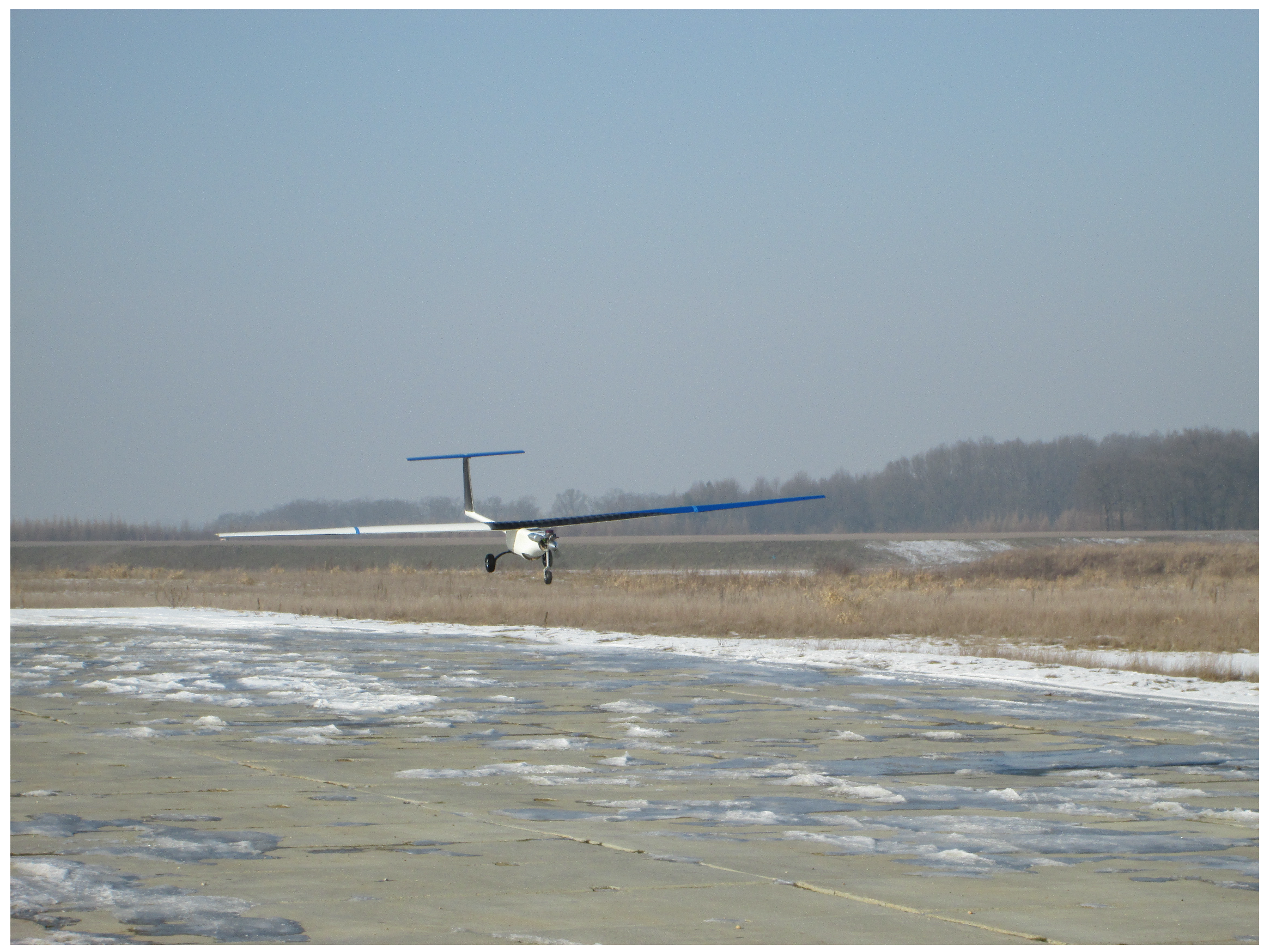
As for publications considering bio-inspired morphing wings at very low Reynolds numbers [14], they usually refer to micro Unmanned Aerial Vehicles (UAVs) (see Figure 1). Anoyoji et al. [15] studied owl-like airfoils for low Reynolds number flights of Micro Air Vehicles (MAVs). The NACA0012 airfoil was compared with a smooth owl-like airfoil for $Re=23,000-60,000$. The authors found that a strong under-camberfor morphing airfoils causes a higher lift force coefficient compared to the NACA0012 airfoil. Another bio-inspired structure for MAVs was researched by Bardera et al. [16]. They conducted three-dimensional studies using the PIV and CFD methods for a stingray-like MAV. Three different morphing stages were examined, and it was concluded that semi-deformation demonstrated the best aerodynamic improvement. Tamai et al. [17] proposed a flexible-membrane airfoil for an MAV. It could change the shape of the wing in flight to adapt to the current conditions like natural flyers do. They investigated the created membrane airfoil using PIV. Majid and Jo [14] investigated morphing wings at a low Reynolds number. They examined nine cases in CFD simulations, achieving an $18.7\%$ increase in the lift-to-drag ratio for the morphing geometry compared to the conventional airfoil. Bardera et al. [6] established morphing geometries that could prevent flow from separation, significantly enhance the lift force coefficient, and reduce turbulence. A technical approach to UAV morphing wings was presented by Dhileep et al. [18]. They investigated a single corrugated variable camber concept and demonstrated that the morphing airfoils exhibited increased the performance compared to the traditional ones. The potential existence of the optimal deflection angle to provide the maximum lift-to-drag ratio for every angle of attack was another important conclusion of this work.

There are also publications considering extremely low Reynolds numbers. Zhu et al. [19] conducted research on a rectangular cylinder for $Re=$ 200–400. They studied the flutter phenomenon of a canonical rectangular cylinder model. Their final conclusion was that studying the behaviour of the vortices is crucial to understanding the flutter phenomenon and that even simple low Reynolds number simulations contain important data that can be utilised for future research on higher Reynolds numbers. Another research work on low Reynolds number was conducted by Liu et al. [20]. They created a model of two cylinders in tandem and studied the fluid forces acting on the model for $Re=$ 75–200. The authors demonstrated the reduction of vortex shedding, as well as the decrease of the fluid forces compared to the extensively researched single-cylinder model.

The airfoil morphing concept went beyond only aviation applications a long time ago. Currently, this is a promising solution raised in every field that uses airfoils or hydrofoils as more energy efficient and having higher aerodynamic performance. Fatiha et al. [21] presented a morphing hydrofoil for ship propeller blades. They established that the hydrofoil shape has a significant impact on hydrodynamic forces, and with morphing, the hydrofoil cavitation phenomenon can be controlled. Remaining in heavy load variations, there is one important subject to consider—wind gusts. For example, waves create hydrokinetic loads on tidal turbines, and strong wind gusts may create potentially dangerous aerodynamic loads on wind turbines. An example of such a treacherous condition is a downburst, in aviation considered very risky during the landing of aircraft and for UAVs. Frant et al. [22] created an aerodynamic state-of-the-art CFD method to model gusts, allowing modelling any speed and direction or time-varying direction of a gust. They conducted aerodynamic wind tunnel tests to validate the numerical model. The results showed that a 10 m/s gust can significantly change the aerodynamic forces and moments acting on the wing. Another numerical model was proposed by Zhou et al. [23]. The authors created a surrogate model for wind turbine wake prediction. The potential of this model enables predicting fluctuating wake structures’ dynamics in hazardous terrain and extreme weather conditions.

Wind turbines are the main objective of current green energy solutions. The aim is to harvest more energy with the lowest possible costs. Thus, the number of wind turbines is growing drastically. Longer blades and higher pylons allow exploiting faster breezes at greater altitudes. This causes higher loads on turbine blades and generates potential construction difficulties. Passive adaptive blades have proven their ability to reduce loads on wind turbine blades in varying weather conditions. Changes in aerodynamic coefficients created by trailing-edge deflection present a linear relation to wind speed [24]. Experimental and numerical approaches to passive adaptive wind turbine blades were presented in Murray’s work [25]. The research revealed a significant reduction of loads for adaptive flexible airfoils compared to rigid blades. Beyene and Peffley [26] conducted wind tests confirming that flexible blades decrease loads to even $10\%$ compared to rigid ones. They concluded that flexible blades adapt better to different load conditions with zero additional costs for harvested energy. The innovative response to the growing problem of high loads on turbine blades could be morphing airfoils. They could also be utilised to support wind turbine rotor braking in a variety of situations. With the development of smart materials and the continuously appearing new technical approaches to morphing airfoils, these active flexible structures could adapt more efficiently to varying weather conditions or hazardous situations and improve efficiency with their tested load reduction and aerodynamic efficiency improvement [27].

Following green energy solutions, morphing airfoils have found their place in tidal turbine applications. Oceanic currents are an unexploited source of green energy with great potential and could seriously strengthen energy security. Hoerner et al. [28] experimented with hydrokinetic vertical-axis or cross-flow tidal turbine (CFTT) morphing blades. They concluded that the flexibility of the camber-morphing airfoil has a significant impact on the wake structure and allows less accidental wake changes over time. A passive–adaptive geometry of airfoils was presented by Castorrini et al. [29]. The authors conducted 2D and 3D FSI simulations of three small rotor geometries, also for fluctuating water flow conditions. The study revealed the computational fluid–structure interaction to have great possibilities for modelling tidal turbine rotors. Present tidal turbines encounter several inconveniences such as current fluctuations caused by waves, large hydrokinetic loads’ inconstancy, or interaction with turbine supports. In their theoretical study, Pisetta et al. [30] discussed morphing blades with such flexibility, for which the load increase from current fluctuations can be reduced by even $99\%$ without affecting the amount of energy harvested.

Another interesting application of morphing airfoil structures is the automotive industry. Flexible structures can create additional passively developed forces for increased grip and enlarged stability in corners. Mishra et al. [31] conducted research on Flexi Wings for Formula 1 race car application. This concept can provide more precise air flow direction adjustment, which enhances manoeuvrability and optimises steering control. The interaction between components can significantly increase or decrease race car performance. Cravero et al. [32] conducted a numerical analysis of the aerodynamic interaction between the front wing and front wheel in a Formula 1 race car. The research revealed that the rotating wheel enhances the aerodynamic performance of the race car’s front section and that swirling flow over the front wing lowers the pressure before the air intake, generating increased air intake efficiency. This phenomenon could be strengthened by the application of a morphing wing structure. Active aerodynamic morphing structures and their ability to change aerodynamic performance could enhance safety during the Brake-In-Turn manoeuvre. Broniszewski and Piechna [33] created an algorithm combining a CFD solver with a car dynamics’ solver. The authors proposed an aerodynamic solution for in-turn braking enhancement by creating additional downforce on the rear wheels and enabling active prevention of control loss during corner braking.

Camber-morphing airfoils are a multidisciplinary subject with an emphasis on aviation. The recognition of the turbulence around morphing structures, as well as creating new camber-morphing airfoils and comparing them to conventional ones are crucial for creating optimal aerodynamic morphing airfoils for aviation [13] as energy solutions [34]. Thus, this paper investigates changes in the aerodynamic efficiency of the airfoils for representative angles of attack and presents the turbulence distribution at very low Reynolds numbers. The main objective of this work is to research a variety of morphing airfoils with different camber deflections. The majority of the literature focuses on very limited camber deflections, and the authors find high cambered morphing airfoils an interesting and insufficiently researched field of aerodynamics. The research was conducted in a two-dimensional way, as for the PIV method, as for CFD simulations. Experiments were performed in a hydrodynamic tunnel using PIV for six airfoil models with various morphing stages. The CFD simulations were obtained using the OpenFOAM software and utilising the k$\omega$-SST turbulence model. The CFD environment was a representation of an experiment conducted in an aerodynamic water tunnel. The lift force coefficients, drag coefficients, and lift-to-drag ratio characteristics are presented.

2. Materials and Methods

2.1. Camber-Morphing Airfoils

The literature presents camber-morphing airfoils in various ways. The deformation could be applied to the leading edge section [35], trailing edge section [36], or both sections of an airfoil [37,38]. The most popular is a continuous camber-morphing trailing edge, as it replaces conventional flaps and is undisturbed by the slit geometry. It is also most suitable for wind or water turbine applications. The authors created an airfoil with $75\%$ camber morphing. The base airfoil was the NACA24012, and a $25\%$ mean aerodynamic chord (MAC) from the leading edge was fixed. Figure 2 presents the morphing airfoil geometries: The Airfoil 1 geometry corresponds to the NACA24012 airfoil. Airfoils 2–6 have variable continuous camber deflections. Airfoil 1 has an initial angle of attack of 0°. Camber-morphing airfoils have the trailing edge moved downwards, and the same as Airfoil 1’s position of the leading edge section, they have different initial angles of attack, as presented in

Table 1. Airfoil dimensions.

Parameter	Airfoil 1	Airfoil 2	Airfoil 3	Airfoil 4	Airfoil 5	Airfoil 6
Chord (c), mm	250	249	246	240	231	221
Initial angle of attack, °	0	7	13	19	26	32

. The geometries were prepared to cover camber deflections from non-cambered (Airfoil 1—NACA24012 airfoil) to fully cambered (Airfoil 6). Between these two airfoils, an additional four were created to cover the whole range of deflections.

Three-dimensional models were created from the prepared two-dimensional airfoil geometries. The models were cut into pieces suitable for a 3D printer. Then, the geometries were printed from polylactic acid (PLA) material using an additive manufacturing method. As this method of printing is imperfect and leaves the surface of the obtained geometry rough, the printed models were first glued from pieces into full models, then coated with plastic primer and aerosol filler. Next, the surface was abraded and polished, then finally coated with paint (Figure 3 and Figure 4).

The experiments in the water tunnel and CFD simulations were performed for every airfoil geometry with a setting angle of 0°. The angle of attack and setting angle coincide only for Airfoil 1 due to the bending of the airfoil and moving the trailing edge downwards, which causes an increase in the initial angle of attack for the morphed airfoils.

2.2. Water Tunnel Experiments

The majority of published articles correspond only to numerical calculations [39]. To fully understand the processes in the wake structure behind the airfoil, it is crucial to perform experiments with the ability to observe emerging turbulence [40]. Hydrodynamic tunnels appear to be the best solution for observing turbulence as water has a density about 800-times greater and a dynamic viscosity 50-times higher than air in a standard atmosphere. Therefore, water has more potential for studying turbulence as it is easier to achieve flow visualisation in a denser environment than in an air aerodynamic tunnel, where the visualisation medium is quickly dispersed [41,42].

2.2.1. Experimental Setup

The experiments were performed in the Rolling Hills Research Corporation hydrodynamic tunnel model 2436 with closed fluid circulation (Figure 5). The test section is a rectangular shape of 1830 mm long, 610 mm wide, and 915 mm deep.

The model was mounted on a three-dimensional support system, enabling active movement of the tested geometry during the experiment. The tunnel is equipped with a thermometer and velocity meter for the fluid flow. The measurement of these two values, in cooperation with computer software, allows one to calculate in time Reynolds number. The water flow is provided by an inverter and controlled in computer software in the range from 0 to 280 mm/s [43,44].

The experiments were performed for flow velocity $v=$ 0.0762 m/s (which corresponds to 3 in) and kinematic viscosity $\nu =8.71\times {10}^{-7}$ m²/s. Calculated from the below-presented equation, the Reynolds number for the representative Airfoil 1 was $Re=$ 21,900.

$$Re=c\ast v/\nu ,$$

(1)

The test section was equipped with two linear lasers synchronised to reduce to minimum shade region around the tested geometry (Figure 6). The high-speed camera was positioned in front of the tested geometry (Figure 7).

2.2.2. Particle Image Velocimetry

Particle Image Velocimetry (PIV) is widely used in the analysis of fluid dynamics [45] and fluid–structure interactions [46]. It is a non-intrusive optical method used for the experimental calculation of fluid in a region of interest. Neutrally buoyant particle seeding is highlighted by the linear laser in the area of analysis (Figure 8).

Images of the illuminated particle patterns are captured by a high-speed camera. Then, the calculations are made, taking into consideration the following two images, and the velocity filed distribution is recorded into one matrix. Further, the mean value of the velocity is calculated based on the following 500 matrices. Taking into consideration the image acquisition frequency (frame per second parameter of the high-speed camera), each of the PIV results represents the mean values of the velocity measured over time for 0.5 s. In our study, we used the high-speed camera with the 250 frames per second setting. The final output of the PIV process is a velocity field representation, as presented in Section 3. This visualisation shows the fluid velocities for all tested airfoils.

The results of the Particle Image Velocimetry (PIV) method depend significantly on the interrogation window size (number of pixels taken in cross-correlation calculation). Smaller interrogation windows yield higher spatial resolution, allowing for the detection of finer flow structures. This is especially important in turbulent flows, in the region of analysis close to the airfoil trailing edge. However, smaller windows also mean fewer particles per window, which affects the accuracy and reliability of the velocity measurements. The size of the interrogation window affects the number of particle image pairs available for cross-correlation analysis within each window. A larger window contains more particle pairs, which improves the statistical reliability of the velocity measurement. However, if the window is too large, it may encompass regions of flow with significantly different velocities, leading to decreased accuracy due to averaging over disparate flow regions.

2.3. Computational Fluid Dynamics Simulations

2.3.1. Mathematical Model

In this study, flow simulations were modelled by solving combinations of steady-state incompressible Navier–Stokes equations given by:

$$\left(\mathbf{u}·\nabla \right)\mathbf{u}=-\nabla \left(p/\rho \right)+\nu {\nabla }^2\mathbf{u},$$

(2)

and the continuity equation is stated as:

$$\nabla ·\mathbf{u}=0$$

(3)

where the fluid velocity vector was deemed as $\mathbf{u}$ = $(u_x,u_y)$, the fluid density is $\rho$, pressure is stated as p, and the kinematic viscosity is labelled as $\nu$. The gravity term is omitted in Equation (2) in order to avoid streaming flow interference [47]. Equations (2) and (3) underwent discretisation through the Finite-Volume Method (FVM) approach. The numerical simulations were computed using OpenFOAM (https://www.openfoam.com/), a C++ open-source toolbox designed primarily for the development of customised numerical solvers [48,49,50]. The simulations conducted in this study employed the semi-implicit method for pressure linked equations (SIMPLE) solver algorithm [51,52,53]. The chosen turbulence model was the k-$\omega$ shear stress transport (SST), which is widely recognised as an industry standard [54,55,56] and combines the strengths of both the Wilcox k-$\omega$ model and the k-$ϵ$ model, utilising a blending function. The convective form of the equations for the steady-state k-$\omega$ SST model is expressed as follows [57]:

$$\begin{array}{c}\nabla ·\left(\mathbf{u}k\right)=\frac{P}{\rho }-{\beta }^{*}\omega k+\nabla ·\left[(\nu +{\sigma }_k{\nu }_t)\nabla k\right]\end{array}$$

(4)

$$\begin{array}{c}\nabla ·\left(\mathbf{u}\omega \right)=\frac{\gamma }{{\mu }_t}P-\beta {\omega }^2+\nabla ·\left[(\nu +{\sigma }_{\omega }{\nu }_t)\nabla \omega \right]+2(1-F_1)\frac{{\sigma }_{\omega 2}}{\omega }\nabla k\nabla \omega \end{array}$$

(5)

where $\rho$ is the fluid density, k is the turbulent kinetic energy, $\omega$ is the specific dissipation rate, $\mathbf{u}$ is the fluid velocity vector, ${\mu }_t$ is the turbulent eddy viscosity, $\nu$ is the kinematic viscosity, ${\nu }_t$ is the turbulent kinematic viscosity, ${\sigma }_k$ is the turbulent Prandtl number for k, ${\sigma }_{\omega }$ is the turbulent Prandtl number for $\omega$, P is the production term, and $F_1$ is the blending function. Variables such as $\beta$, ${\beta }^{*}$, $\gamma$, ${\sigma }_k$, ${\sigma }_{\omega }$, and ${\sigma }_{\omega 2}$ are constants.

2.3.2. Aerodynamic Coefficients

The lift, drag, and momentum coefficients are defined as follows:

$$\begin{array}{c}{C}_L=\frac{F_L}{A_{ref}·p_d}\end{array}$$

(6)

$$\begin{array}{c}{C}_D=\frac{F_D}{A_{ref}·p_d}\end{array}$$

(7)

$$\begin{array}{c}{C}_M=\frac{M}{A_{ref}·l_{ref}·p_d}\end{array}$$

(8)

$$\begin{array}{c}{p}_d=\frac{{\rho }_{ref}·{U_{mag}}^2}{2}\end{array}$$

(9)

where $F_L$ and $F_D$ are forces perpendicular to and parallel with the direction of the flow, M is the moment acting around the axis of rotation, $A_{ref}$ corresponds to the total wing surface area, and $l_{ref}$ in this case is the chord length. Dynamic pressure $p_d$ is defined by the reference density ${\rho }_{ref}$ and the velocity magnitude $U_{mag}$. For incompressible cases, Equations (6)–(8) are solved using the kinematic pressure $p_k=p_d/\rho$ [58,59].

2.3.3. Discretisation Schemes

The discretisation schemes are discussed based on the OpenFOAM source code. The summary and accuracies [60,61,62] of the selected schemes are provided in

Table 2. Summary of discretisation schemes used in the study.

Schemes	Terms	Scheme Type	Accuracy
Time	default	steadyState	time derivative set to 0
Gradient	default	Gauss linear	2nd order, unbounded
	$\nabla \mathbf{u}$	cellLimited Gauss linear 1	2nd-order, cell-limited version
Divergence	default	none;	specified for each term
	$\nabla ·\left(\varphi \mathbf{u}\right)$	bounded Gauss linearUpwind grad(U)	2nd-order, bounded
	$\nabla ·\left(\varphi k\right)$	bounded Gauss upwind	1st-order, bounded
	$\nabla ·\left(\varphi \omega \right)$	bounded Gauss upwind	1st-order, bounded
	$\nabla ·\left(({\nu }_{\mathrm{Eff}}·{\mathrm{dev}}^2\left(\mathrm{T}(\nabla \mathbf{u})\right))\right)$	Gauss linear	2nd-order, unbounded
Laplacian	default	Gauss linear corrected	2nd-order, unbounded
Interpolation	default	linear	2nd-order, unbounded
Surface normal gradient	default	corrected	2nd-order

. The steadyState time scheme sets temporal derivative contributions to zero. Gauss linear is the default gradient scheme that was used. The Gauss entry specifies the standard finite-volume discretisation with Gaussian integration, which requires the interpolation of the values from the cell centres to the face centres. The interpolation scheme is then given by the linear interpolation or central differencing. The discretisation of the velocity gradient was overridden with the cellLimited scheme, which improves boundedness and stability. The divergence schemes contain both advection terms and other terms, which are often diffusive in nature. The non-advective terms used the Gauss integration with linearUpwind or upwind interpolation. The bounded variant of the Gauss scheme helps maintain boundedness and promotes better convergence. The surface normal gradient is evaluated at a cell face.

The calculation is 2nd-order accurate, if the vector connecting the cell centres is orthogonal to the face (orthogonal scheme) or an explicit non-orthogonal correction has been added (corrected scheme), which is recommended for maximum non-orthogonality $\le {75}^{\circ }$. As meshes in this study had a maximum non-orthogonality of ${35}^{\circ }$, this exact term was used. The Gauss scheme is the only choice of Laplacian discretisation. In all cases, the linear scheme was used for interpolation of the diffusivity. The cases used the same array of surface normal gradient schemes based on the maximum non-orthogonality in the mesh, as described above. The interpolation schemes contain terms that are interpolations of values typically from cell centres to face centres. There are numerous interpolation schemes in OpenFOAM, but the linear interpolation is the most frequently used [60,61,62]. While the majority of schemes were 2nd-order accurate, $\nabla ·\left(\varphi k\right)$ and $\nabla ·\left(\varphi \omega \right)$ used 1st-order schemes in order to provide better stability of the simulations, which was recommended due to their diffusive nature.

2.3.4. Geometry for the CFD Case Study

The geometries analysed in the study are shown in Figure 2. Airfoil chords varied between $c=221$ and 250 mm and were differentiated by camber lines. More detailed information on the airfoil geometries can be found in Table 1.

2.3.5. Computational Domain

The determination of computational domain dimensions conventionally relies on the geometric characteristics of the subject of investigation. In the context of airfoils and wings, this parameter is typically defined by the mean aerodynamic chord (MAC) or simply the chord length, denoted as c. The exact size of the computational domain needed to accurately capture the physics varies depending on the problem. However, there are general guidelines for determining the domain dimensions. For 2D subsonic aerodynamic simulations, it is recommended that the domain length should be 5c at minimum or ideally ≥ 100c [63,64,65]. Nonetheless, this is a broadly generalised guideline for external aerodynamics, with Reynolds numbers reflecting real-world flow conditions. In addition to these general prerequisites, feasibility and computing power must also be taken into account. Under appropriately chosen boundary conditions, the determination of the computational domain size, in terms of external aero- or hydrodynamics, focuses on one primary consideration: the magnitude of error resulting from the domain boundaries positioned too closely to the studied object [66].

As the CFD method served merely as a supportive research tool in this preliminary study of morphing airfoils and considering that the flow conditions were characterised by low Reynolds numbers, very low flow velocity, and water as the medium, which did not impose real external aerodynamic demands, we opted for smaller domain dimensions of $\mathit{30}\mathit{c}$. This decision represents an acceptable trade-off, balancing potential errors as highlighted on NASA’s website [66] and in other studies [67]. There is a substantial number of airfoil studies that propose similar domain dimensions, as exemplified in [68,69].

The airfoils were meshed with the use of the mesh utility named snappyHexMesh, which comes with the OpenFOAM package. This tool produces hex-dominant meshes from triangulated geometries and adds layers during the concluding stage of the meshing process. As the primary focus of the study was centred on Particle Image Velocimetry (PIV) experiments, a decision was made to prioritise cell refinement in the near-airfoil region to deliver high-resolution results, which would serve as a reliable basis for comparison between the images extracted from the PIV results and CFD simulations. The development of the numerical mesh was divided into two parts: the computational domain and the circular shape containing the airfoil. The computational domain mesh had an opening where the numerical mesh of the airfoil was subsequently inserted and stitched together. This solution will allow the easy rotation of the airfoil in future wide-rangenumerical simulations. These methods are widely known and often utilised by researchers, as exemplified in [69,70].

Figure 9 illustrates the conceptual shape of the computational domain with marked distances and dimensions.

The airfoil chord length is denoted as $\mathit{c}$ and is provided in Table 1. The size of the domain was specified as $\mathit{10}\mathit{c}$ for the front, top, and bottom of the airfoil and $\mathit{20}\mathit{c}$ behind the airfoil. This resulted in dimensions of $\mathit{30}\mathit{c}$ along the x-axis and $\mathit{20}\mathit{c}$ along the y-axis. A smaller dimension was selected for the y-axis due to the consistent inflow direction across the cases. Specifically, the angle of attack will be manipulated by rotating the inner cell zone containing the airfoil. Consequently, the predominant flow direction remains along the x-axis until it reaches the airfoil. The dimensions in the y-axis direction were tailored to accommodate flow deflection and turbulent effects induced by the airfoil. Bearing this consideration in mind, it was found that employing 20c dimensions downstream of the airfoil adequately captured the resulting flow pattern.

The z-axis dimension is absent in this study as the cases were two-dimensional (2D). The centre point of the mesh, $(x,y)=(0,0)$, was specified as the airfoil’s aerodynamic centre. The rotating cell zone had a diameter of $\mathit{2}\mathit{c}$ to accommodate the airfoil and proper cell refinement zones around it. The angle of attack could be obtained by rotating the inner cell zone, which contained the airfoils. The numerical grid was regularly refined in the area around the airfoils and in their slipstream. Additionally, the region near the airfoils also underwent refinement. Each cell level step had a blending function of seven cells in between the cell levels. In the arbitrary mesh interface (AMI) region, the meshes had one refinement function of level 5 at a distance of 0.05 m from the airfoil geometry. The airfoil silhouette was represented by a surface refinement cell level of 6, which translates to a cell edge length of $1.56\times {10}^{-4}$ m.

The length of the edges of the base cells was 0.01 m, and the cell refinement in the domain was performed with an expansion factor $E=\frac{{\delta }_t}{{\delta }_b}$, where ${\delta }_t$ is the ratio of the cell height at the top of the grid block to the cell height at the bottom of the grid block ${\delta }_b$. For the lower grid block, $E_b=4$, and for the upper grid block $E_t=\frac{1}{4}$. The developed 2D numerical grids comprised around 3,370,000 cells. To represent the viscous sublayer, $n=25$ layers with an inflation factor of $\delta =1.2$ were generated. The thickness of the first layer was $y=7.862\times {10}^{-7}$ m, ensuring a dimensionless wall distance $y+<1$ for all geometries (Figure 10). Key features of the numerical grids are presented in Figure 11.

2.3.6. Flow Characteristics and Boundary Conditions

Numerical studies simulated the 2D hydrodynamics around the airfoil geometries in a steady state. The flow was deemed as subsonic with very low Mach or Reynolds numbers. The material settings were the same as is the case for water at 26.3 °C. The material was a single-phase, non-reacting, and incompressible Newtonian fluid. The flow characteristics can be found in

Table 3. Flow characteristics.

Label	Quantity
Type	Steady-state 2D hydrodynamics
Fluid	Newtonian, single-phase, incompressible
Material	Water at 26.3 °C
Water density	$\rho$ = $996.784$ $\frac{\mathrm{kg}}{{\mathrm{m}}^3}$
Kinematic viscosity of fluid	$\nu$ = $8.71\times {10}^{-7}$ $\frac{{\mathrm{m}}^2}{\mathrm{s}}$
Reynolds number	Re = 19,400–21,900
Streamwise far-field flow speed	U = 0.0762 $\frac{\mathrm{m}}{\mathrm{s}}$
Characteristic length (airfoil chord)	c = 0.231–0.25 m

.

Equations (11)–(13) [71] were used to calculate the initial values of k and $\omega$.

Table 4. Boundary conditions for velocity, pressure, and kinematic viscosity.

BC/Field	u, $\frac{\mathbf{m}}{\mathbf{s}}$	p, $\frac{{\mathbf{m}}^2}{{\mathbf{s}}^2}$	${\mathit{\nu }}_{\mathit{t}},$$\frac{{\mathbf{m}}^2}{\mathbf{s}}$
Inlet	$u_x=0.0762$	$\frac{\partial p}{\partial n}=0$	solved by k-$\omega$ model
Outlet	$\frac{\partial u}{\partial n}=0$ and $u_x=0.0762$	$p=0$	solved by k-$\omega$ model
Top/bottom	cyclic	cyclic	empty
Left/right	empty	empty	cyclic
AMI domain/airfoil	cyclic	cyclic	cyclic
Airfoil	$u=0$	$\frac{\partial p}{\partial n}=0$	${\nu }_{t_{wall}}$ function

and

Table 5. Boundary conditions for turbulent kinetic energy and turbulence specific dissipation rate.

BC/Field	k, $\frac{{\mathbf{m}}^2}{{\mathbf{s}}^2}$	$\mathit{\omega },$$\frac{1}{\mathbf{s}}$
Inlet	$\frac{\partial k}{\partial n}=0$ and $k=8.71\times {10}^{-7}$	$\frac{\partial \omega }{\partial n}=0$ and $\omega =0.0077$
Outlet	$\frac{\partial k}{\partial n}=8.71\times {10}^{-7}$	$\frac{\partial \omega }{\partial n}=0$ and $\omega =0.0077$
Left/right	empty	empty
Top/bottom	cyclic	cyclic
AMI domain/airfoil	cyclic	cyclic
Airfoil	$k_{wall}$ function	${\omega }_{wall}$ function

represent the boundary conditions for the steady-state simulations. The velocity components $u_x$, $u_y$ are calculated from the velocity magnitude u and angle of attack $\alpha$. The equations for k, $\omega$, and ${\omega }_{wall}$ were taken from the OpenFOAM user guide [71] and are presented below:

$$\begin{array}{c}(u_x,u_y)=(\mathbf{u}cos\alpha ,\mathbf{u}sin\alpha )\end{array}$$

(10)

$$\begin{array}{c}k=\frac{3}{2}{\left(\mathbf{u}I\right)}^2\end{array}$$

(11)

$$\begin{array}{c}\omega =\frac{k^{0.5}}{C_{\mu }^{0.25}·L}\end{array}$$

(12)

$$\begin{array}{c}{\omega }_{wall}=\frac{6\nu }{{\beta }_1{y}^2}\end{array}$$

(13)

where I is the turbulence intensity, u is the velocity magnitude inside the domain, $C_{\mu }$ is a constant of 0.09, L is the reference length scale, $\nu$ is the kinematic viscosity, ${\beta }_1$ is a constant of 0.075, and y is the wall normal distance.

The convergence criterion for steady-state simulations utilised residual control for velocities $u_x|u_y\le 1\times {10}^{-6}$, kinematic pressure $p\le 1\times {10}^{-6}$, turbulent kinetic energy, and the specific dissipation rate $k|omega\le 1\times {10}^{-6}$. This meant that the simulations automatically stopped when all residuals reached the specified threshold. If these criteria were not satisfied, a backup convergence criterion was set at a total number of iterations $n=\mathrm{35,000}$.

3. Results and Discussion

In this section, the results of the obtained experiments and simulations are discussed. As explained in Section 2.3.5, the main focus of the study was centred on the PIV experimental approach. CFD simulations were performed to create an aerodynamic coefficient characteristics’ trend. For that reason, the medium remained water and the boundary conditions, such as velocity, remained unchanged. The validation of the numerical model was based on the velocity distribution. The obtained CFD results were of good quality and good enough to provide sufficient aerodynamic coefficient numerical results, especially for the preliminary research this work presents. Nevertheless, the authors present some insight into the differences between experimental and computational velocity distribution results.

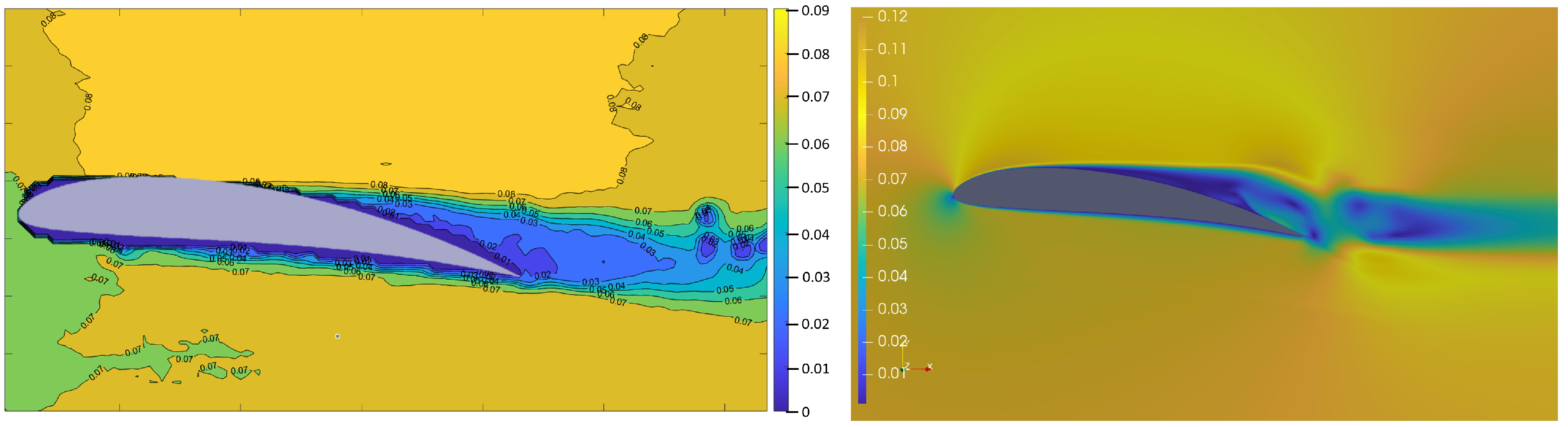
In the figures (Figure 12, Figure 13, Figure 14, Figure 15, Figure 16 and Figure 17), the PIV and CFD results are presented. The shapes of the airfoils were inserted into PIV results to clarify the actual airfoil shape in every condition, as the shaded region in PIV varies and is not always identical to the tested geometry, especially in the area in front of the leading edge.

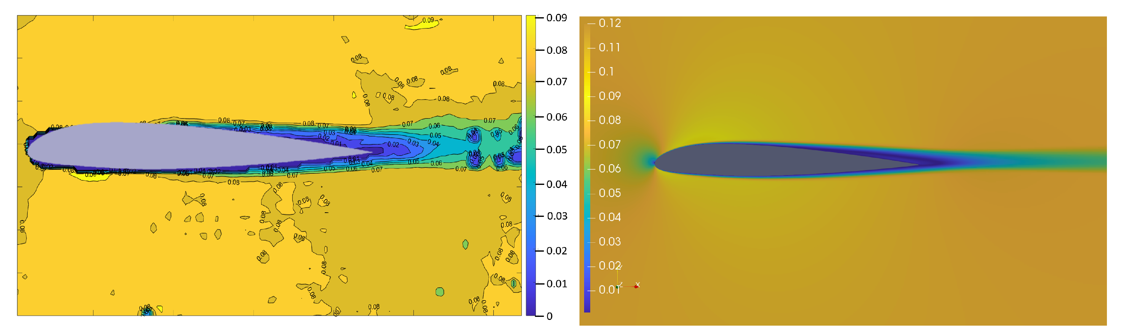
Figure 12 presents the velocity distribution for the NACA24012 airfoil, in this article, named Airfoil 1. As one can see, the velocity distribution is in the same range for both graphic results, and the laminar flow from the CFD method is less turbulent. Even for low Reynolds numbers and non-morphed airfoils, the wake structure behind the airfoil is turbulent, which is clearly visible in the discussed figure on the PIV result. The CFD results are numerical simulations taking ideal conditions and simplifying the environmental models, as the PIV method is an experimental method conducted in a real water tunnel. This simple comparison confirms the demand for an experimental approach to the turbulence study.

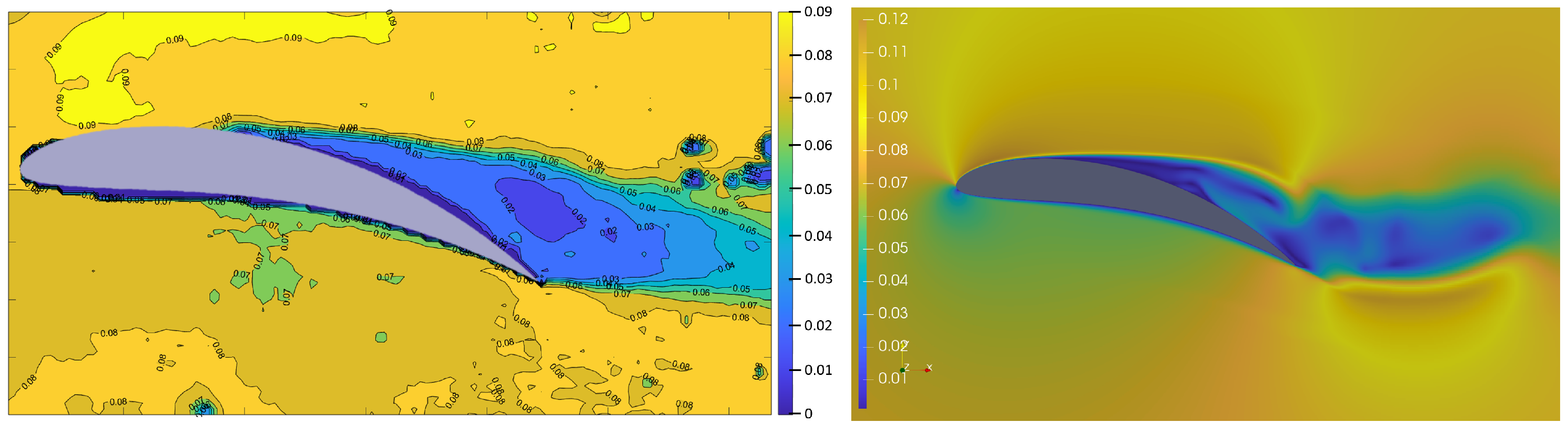
In Figure 13 and Figure 14, the CFD results, there are two areas of increased velocity, one above the airfoil and a second behind the trailing edge. The PIV results show a similar distribution of velocity, but in the CFD results, the velocity in this area is higher. The turbulence is comparable, taking into consideration that the PIV results are average values from 500 camera frames, and the CFD result is presented for specific iterations. Despite the clearly visible differences between the presented results, the velocity distribution and turbulence distribution are comparable, which enables the validation of the CFD results.

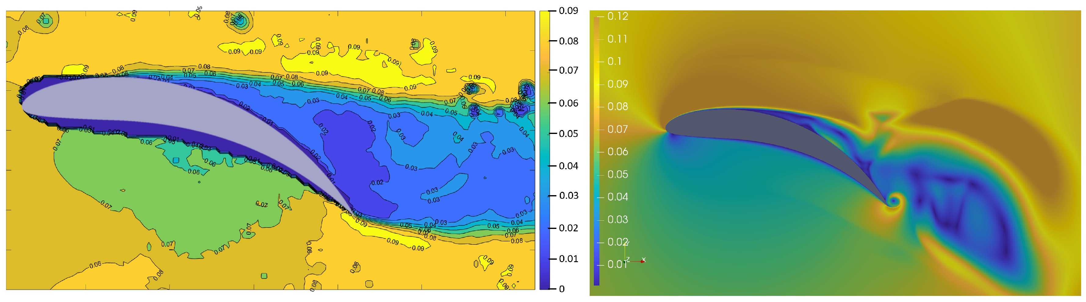
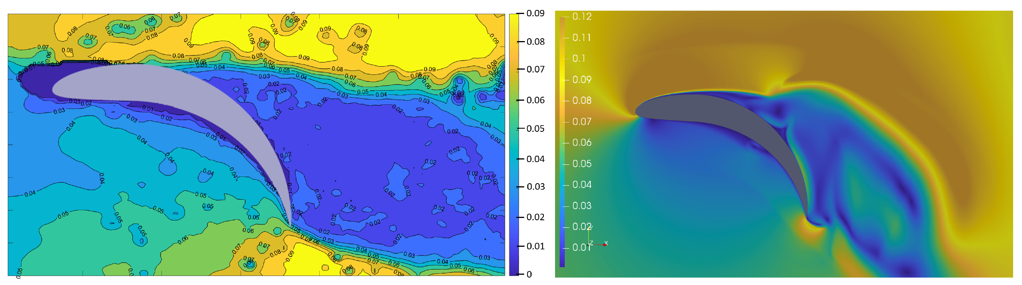
In Figure 15, again, there is an area of increased velocity above the airfoil that spreads widely behind the airfoil geometry. This occurs for both the CFD and PIV results, and only the values of the maximum velocity differ. The wake structure is moved downwards in the CFD result, due to the increased velocity area behind the airfoil. Behind the trailing edge, in the PIV result, there is an increase in the velocity, and for the CFD results, this increase has a circular shape. As the PIV results’ values were averaged and show only the velocity distribution and not the eddy circulations, the actual flow is wrapping around the trailing edge, as shown in the CFD result.

For Airfoil 5’s graphic results (Figure 16), they are similar to the previous areas of increased velocity. One is placed above the airfoil and other behind the trailing edge of the airfoil. The increased velocity area behind the trailing edge is longer and wider and the wake structure is greater compared to Airfoil 4’s results. On the upper side of the airfoil in both results, there is an area of increased velocity, suggesting the indication of a large eddy in this area. The upper side of the wake structure in the CFD results is slightly moved downwards compared to the PIV result.

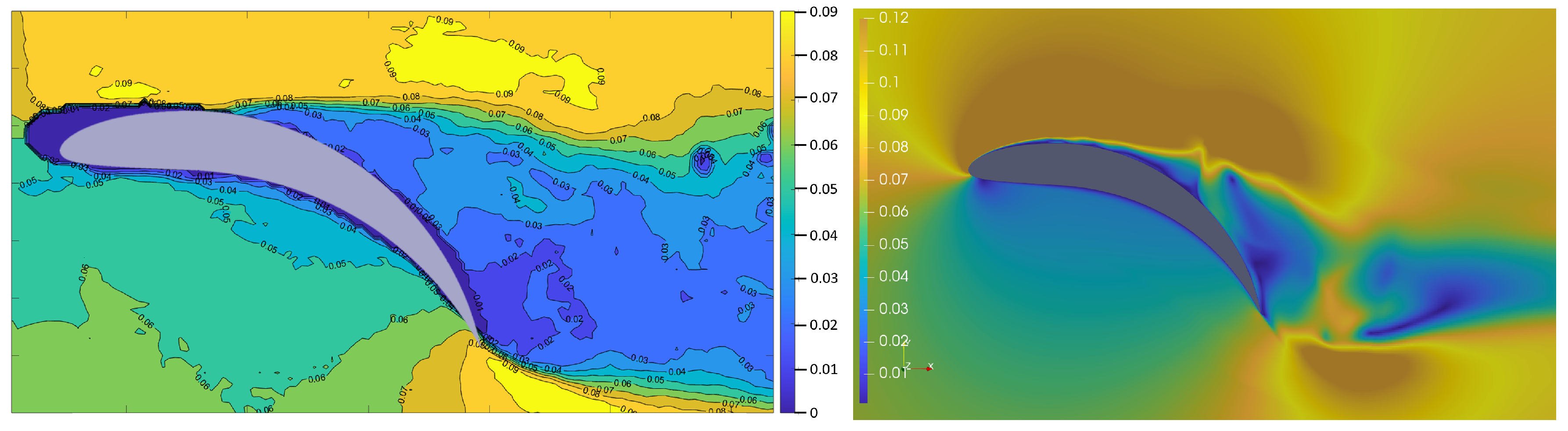
The fully morphed airfoil’s geometry results are presented in Figure 17. The flow is fully separated, and the areas of increased velocity above the airfoil and behind the trailing edge present the maximum region. In the CFD result, the wake structure is significantly moved downwards for this specific iteration, as it fluctuates upwards and downwards in the real condition. In the middle of the airfoil’s upper surface, there is a clearly visible eddy in both graphic results.

Relating to all above-mentioned graphic results, the velocity distribution under the airfoils is highly comparable and adequate for both research methods. The wake structure has similar eddy structures for both conducted research methods. The CFD results are characterised by slightly higher maximum velocity values, but their distribution over the presented region is adequate. The wake structure is raising proportionally to the camber deflection of the airfoil. The two mean regions of increased velocity are recognised, one above the rear side of the airfoil and the other one behind the trailing edge. These regions are also rising with camber deflection. The boundary layer separation occurs at the same point for every airfoil geometry for both experiment methods. The CFD results are similar to the PIV results in the eddy distribution, though the fluctuation of the wake structure in the CFD results causes the wake structure to descend. This occurs more intensively with the increase in the camber deflection.

In the PIV results, one can notice small eddies behind the airfoil for every airfoil geometry. These structures do not appear in the CFD results, as CFD creates smoother results. During experiments, many eddies were visible in the turbulence region behind the airfoil. The CFD results are not as clearly visible due to the simplifications, by which the computational solutions are affected.

The differences between the PIV and CFD results described above are a representation of the demand for an experimental approach to flow research. Nevertheless, the similarities of both methods are clearly visible and precisely described to ensure the validation of the numerical model. The CFD numerical results were obtained and are presented in

Table 6. Computational fluid dynamic simulations’ results.

Geometry	Lift Force Coefficient, Cl, -	Drag Coefficient, Cd, -	Pitching Moment Coefficient, Cm, -	Lift-to-Drag Ratio, L/D, -
Airfoil 1	0.0186	0.0296	0.0047	0.63
Airfoil 2	1.0193	0.2632	0.2270	3.87
Airfoil 3	1.3994	0.6259	0.2917	2.24
Airfoil 4	2.2312	1.2223	0.4082	1.83
Airfoil 5	2.4449	2.0139	0.5768	1.21
Airfoil 6	1.9709	2.5618	0.7049	0.77

. A graphic representation of the results is presented in Figure 18.

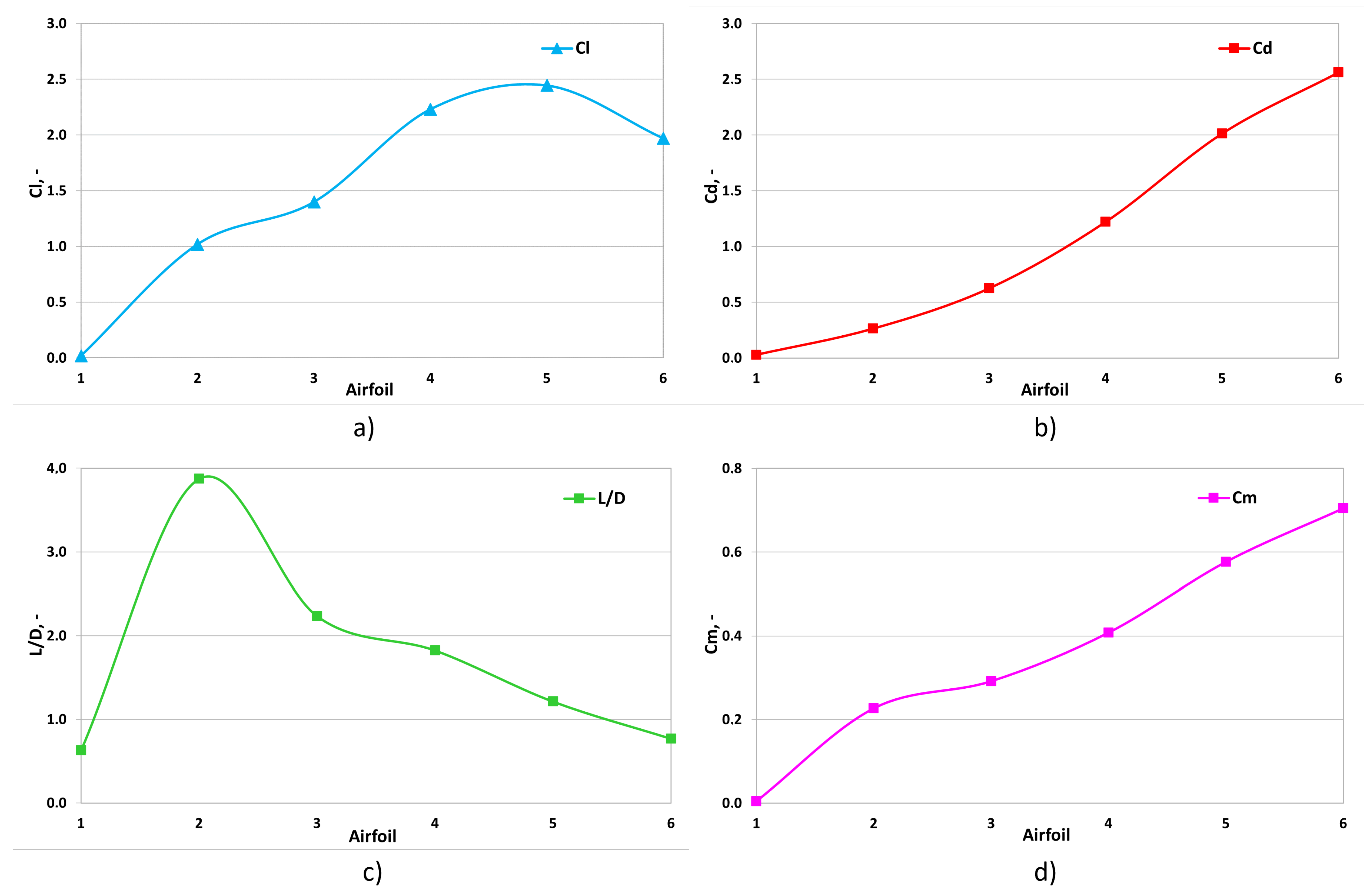
Figure 18a shows the lift force coefficient characteristics for all geometries. The increase in the lift force coefficient occurs for Airfoils 1 to 5, then it slightly descends for Airfoil 6.

The drag coefficient (Figure 18b) increases with the increase in camber deflection for all geometries. As demonstrated above, the wake structure behind the airfoil rises with camber deflection, and greater turbulence implies higher drag.

The lift-to-drag ratio is a very useful value; it is the relation between the lift force coefficient and drag coefficient. It reveals the maximum amount of aerodynamic energy an airfoil is capable of generating. For an aircraft, it would be the distance the aircraft is capable of flying from 1000 m in standard atmosphere ideal conditions. Camber-morphing airfoils with slight camber deflection are usually characterised by better aerodynamic characteristics. Figure 18c shows that the highest lift-to-drag ratio appears for Airfoil 2, a slightly cambered one, as the generated drag is still low and even marginal camber deflection generates high values of lift. Behind Airfoil 2, this characteristic drops significantly due to a lower difference in the increase in the lift force coefficient than for Airfoil 2 and an increase in the drag coefficient. For Airfoils 3 to 6, the lift-to-drag ratio descends linearly as the turbulence region and drag enhance drastically.

Every camber deflection provokes the pitching moment to increase. Aircraft pilots experience this phenomenon when the flaps are extended during every approach to landing. The pitching moment coefficient value for every geometry is presented in Figure 18d. The pitching moment increases nearly linearly with the camber deflection of an airfoil.

4. Conclusions

In this paper, the authors presented and discuss substantial camber-morphing airfoil geometry experiments. The research was conducted with two methods: experimental in the water tunnel using the PIV method for velocity distribution representation and computational using CFD software for obtaining the coefficients and graphic velocity distribution representation.

This work presents preliminary research with the main objective to study a variety of camber-morphing airfoils with a wide range of camber deflections.

The CFD and PIV velocity distribution results exhibited significant similarities, which enables the validation of the numerical model. The aerodynamic coefficients were consistent with the predictions’ trends. It can be stated that Airfoil 2 had the best aerodynamic performance. Most research pursues creating the optimal airfoil with the highest lift force coefficient and lowest drag coefficient. It was demonstrated that camber-morphing airfoils can create drastic amounts of drag, retaining smooth and continuous surfaces. This could be a solution for micro UAV aircraft to reduce landing speed, without the necessity of installing wing mechanisation, which disturbs the airflow over the wing surface. Highly cambered airfoils can significantly reduce the landing distance, as they create massive amounts of drag, maintaining high lift.

However, airfoils with higher camber deflections can be utilised in various environments. This could be advantageous for wind turbines or tidal turbine engineers struggling with load reduction in hazardous atmospheric conditions. As highly cambered morphing airfoils create substantial drag, they could be utilised for rotor braking.

The CFD results were comparable, but they were not identical to the experimental results. As the simulations were performed in the exact environment as the experiments in the water tunnel, the simulations provided accurate and comparable results, but the differences were visible. This is a confirmation of the persisting need for an experimental approach to wake structures and turbulence research in the era of numerical simulations.

The next step of this preliminary research will be conducting experiments and numerical simulations on a wider range of angles of attack. The authors would like to obtain the full aerodynamic characteristics of the presented camber-morphing airfoils and to perform calculations correlating high amounts of produced drag with loads acting on turbine rotors and aircraft wings.

Substantial camber-morphing airfoils may be implemented in various applications from diverse fields. Though their applications are limited due to the limited abilities of current mechanical features, there remains demand for conducting aerodynamic research and for verifying different aerodynamic solutions for future use. The authors pushed the morphing airfoil concept a step further, creating a geometry that produces drag instead of decreasing it while maintaining a continuous surface. It is a solution with great potential and perspectives for further investigation.

References

1. Weisshaar, T.A. Morphing aircraft systems: Historical perspectives and future challenges. J. Aircr. 2013, 50, 337–353. [Google Scholar] [CrossRef]
2. Ozbek, E.; Ekici, S.; Karakoc, T.H. Unleashing the Potential of Morphing Wings: A Novel Cost Effective Morphing Method for UAV Surfaces, Rear Spar Articulated Wing Camber. Drones 2023, 7, 379. [Google Scholar] [CrossRef]
3. Dharmdas, A.; Patil, A.Y.; Baig, A.; Hosmani, O.Z.; Mathad, S.N.; Patil, M.B.; Kumar, R.; Kotturshettar, B.B.; Fattah, I.M.R. An Experimental and Simulation Study of the Active Camber Morphing Concept on Airfoils Using Bio-Inspired Structures. Biomimetics 2023, 8, 251. [Google Scholar] [CrossRef] [PubMed]
4. Di Luca, M.; Mintchev, S.; Heitz, G.; Noca, F.; Floreano, D. Bioinspired morphing wings for extended flight envelope and roll control of small drones. Interface Focus 2017, 7, 20160092. [Google Scholar] [CrossRef]
5. Ahmad, D.; Ajaj, R.M. A Multiaxial Fracture of Ecoflex Skin with Different Shore Hardness for Morphing Wing Application. Polymers 2023, 15, 1526. [Google Scholar] [CrossRef] [PubMed]
6. Bardera, R.; Rodríguez-Sevillano, Á.; García-Magariño, A. Aerodynamic investigation of a morphing wing for micro air vehicle by means of PIV. Fluids 2020, 5, 191. [Google Scholar] [CrossRef]
7. Abdessemed, C.; Bouferrouk, A.; Yao, Y. Effects of an unsteady morphing wing with seamless side-edge transition on aerodynamic performance. Energies 2022, 15, 1093. [Google Scholar] [CrossRef]
8. Giuliani, M.; Dimino, I.; Ameduri, S.; Pecora, R.; Concilio, A. Status and Perspectives of Commercial Aircraft Morphing. Biomimetics 2022, 7, 11. [Google Scholar] [CrossRef]
9. Sofla, A.; Meguid, S.; Tan, K.; Yeo, W. Shape morphing of aircraft wing: Status and challenges. Mater. Des. 2010, 31, 1284–1292. [Google Scholar] [CrossRef]
10. Nguyen, N.; Kaul, U.; Lebofsky, S.; Ting, E.; Chaparro, D.; Urnes, J. Development of variable camber continuous trailing edge flap for performance adaptive aeroelastic wing. Proc. SAE AeroTech Congr. Exhib. 2015, ARC-E-DAA-TN25273. [Google Scholar] [CrossRef]
11. Ting, E.; Dao, T.; Nguyen, N.T. Aerodynamic load analysis of a variable camber continuous trailing edge flap system on a flexible wing aircraft. In Proceedings of the 56th AIAA/ASCE/AHS/ASC Structures, Structural Dynamics, and Materials Conference, Kissimmee, FL, USA, 5–9 January 2015; p. 1839. [Google Scholar]
12. Ting, E.; Chaparro, D.; Nguyen, N.; Fujiwara, G.E. Optimization of variable-camber continuous trailing-edge flap configuration for drag reduction. J. Aircr. 2018, 55, 2217–2239. [Google Scholar] [CrossRef]
13. Jo, B.W.; Majid, T. Aerodynamic analysis of camber morphing airfoils in transition via computational fluid dynamics. Biomimetics 2022, 7, 52. [Google Scholar] [CrossRef] [PubMed]
14. Majid, T.; Jo, B.W. Comparative aerodynamic performance analysis of camber morphing and conventional airfoils. Appl. Sci. 2021, 11, 10663. [Google Scholar] [CrossRef]
15. Anyoji, M.; Wakui, S.; Hamada, D.; Aono, H. Experimental study of owl-like airfoil aerodynamics at low Reynolds numbers. J. Flow Control Meas. Vis. 2018, 6, 185. [Google Scholar] [CrossRef]
16. Bardera, R.; Rodríguez-Sevillano, Á.A.; Barroso, E. Numerical and Experimental Study of Aerodynamic Performances of a Morphing Micro Air Vehicle. Appl. Mech. 2021, 2, 442–459. [Google Scholar] [CrossRef]
17. Tamai, M.; Murphy, J.; Hu, H. An experimental study of flexible membrane airfoils at low Reynolds numbers. In Proceedings of the 46th AIAA Aerospace Sciences Meeting and Exhibit, Reno, NV, USA, 7–10 January 2008; p. 580. [Google Scholar]
18. Dhileep, K.; Kumar, D.; Vigneswar, P.G.; Soni, P.; Ghosh, S.; Ali, S.F.; Arockiarajan, A. Aerodynamic study of single corrugated variable-camber morphing aerofoil concept. Aeronaut. J. 2022, 126, 316–344. [Google Scholar] [CrossRef]
19. Zhu, Q.; Zhou, L.; Wen, J.; Liu, T.; Zhang, J.; Tang, H.; Zhang, H. Laminar flow over a rectangular cylinder experiencing torsional flutter: Dynamic response, forces and coherence modes. Phys. Fluids 2023, 35, 1–49. [Google Scholar] [CrossRef]
20. Liu, Z.; Zhou, L.; Tang, H.; Wang, Z.; Zhao, F.; Ji, X.; Zhang, H. Primary instability, sensitivity and active control of flow past two tandem circular cylinders. Ocean Eng. 2024, 294, 116863. [Google Scholar] [CrossRef]
21. Fatiha, M.A.; Augier, B.; Deniset, F.; Casari, P.; Astolfi, J.A. Morphing hydrofoil model driven by compliant composite structure and internal pressure. J. Mar. Sci. Eng. 2019, 7, 423. [Google Scholar] [CrossRef]
22. Frant, M.; Kachel, S.; Maślanka, W. Gust Modeling with State-of-the-Art Computational Fluid Dynamics (CFD) Software and Its Influence on the Aerodynamic Characteristics of an Unmanned Aerial Vehicle. Energies 2023, 16, 6847. [Google Scholar] [CrossRef]
23. Zhou, L.; Wen, J.; Wang, Z.; Deng, P.; Zhang, H. High-fidelity wind turbine wake velocity prediction by surrogate model based on d-POD and LSTM. Energy 2023, 275, 127525. [Google Scholar] [CrossRef]
24. Cavens, W.D.; Chopra, A.; Arrieta, A.F. Passive load alleviation on wind turbine blades from aeroelastically driven selectively compliant morphing. Wind Energy 2021, 24, 24–38. [Google Scholar] [CrossRef]
25. Murray, R. Passively Adaptive Tidal Turbine Blades: Design Methodology and Experimental Testing. Ph.D. Thesis, Dalhousie University, Halifax, NS, Canada, 2016. [Google Scholar]
26. Beyene, A.; Peffley, J. A morphing blade for wave and wind energy conversion. In Proceedings of the OCEANS 2007-Europe, Aberdeen, Scotland, 18–21 June 2007; pp. 1–6. [Google Scholar]
27. Lachenal, X.; Daynes, S.; Weaver, P.M. Review of morphing concepts and materials for wind turbine blade applications. Wind Energy 2013, 16, 283–307. [Google Scholar] [CrossRef]
28. Hoerner, S.; Kösters, I.; Vignal, L.; Cleynen, O.; Abbaszadeh, S.; Maître, T.; Thévenin, D. Cross-flow tidal turbines with highly flexible blades—Experimental flow field investigations at strong fluid–structure interactions. Energies 2021, 14, 797. [Google Scholar] [CrossRef]
29. Castorrini, A.; Barnabei, V.F.; Corsini, A.; Rispoli, F.; Takizawa, K.; Tezduyar, T.E. Computational Fluid–Structure Interaction Analysis of Passive Adaptive Blades in Turbomachinery Applications. In Frontiers in Computational Fluid-Structure Interaction and Flow Simulation: Research from Lead Investigators Under Forty-2023; Springer: Berlin/Heidelberg, Germany, 2023; pp. 33–58. [Google Scholar]
30. Pisetta, G.; Le Mestre, R.; Viola, I.M. Morphing blades for tidal turbines: A theoretical study. Renew. Energy 2022, 183, 802–819. [Google Scholar] [CrossRef]
31. Mishra, S.; Singh, S.; Sharma, S.; Bhardwaj, M. Flexi wings: An innovative approach for the future of material science with an aerodynamic influence in motorsport engineering. Int. J. Mech. Eng. 2022, 7, 1193–1202. [Google Scholar]
32. Cravero, C.; Marsano, D. Computational investigation of the aerodynamics of a wheel installed on a race car with a multi-element front wing. Fluids 2022, 7, 182. [Google Scholar] [CrossRef]
33. Broniszewski, J.; Piechna, J.R. Fluid-structure interaction analysis of a competitive car during brake-in-turn manoeuvre. Energies 2022, 15, 2917. [Google Scholar] [CrossRef]
34. Jing, M.; Jinglei, X.; Rui, G.; Kunyuan, Z. PIV Experimental Study of A 2-D Wind Turbine Airfoil under Different Re Number. In Proceedings of the 46th AIAA/ASME/SAE/ASEE Joint Propulsion Conference & Exhibit, Nashville, TN, USA, 25–28 July 2010; p. 6513. [Google Scholar]
35. Zi, K.; Daochun, L.; Tong, S.; Xiang, J.; Zhang, L. Aerodynamic characteristics of morphing wing with flexible leading-edge. Chin. J. Aeronaut. 2020, 33, 2610–2619. [Google Scholar]
36. Shi, X.; Yang, Y.; Wang, Z.; Zhang, S.; Sun, X.; Feng, W. Design and Shape Monitoring of a Morphing Wing Trailing Edge. Aerospace 2023, 10, 127. [Google Scholar] [CrossRef]
37. Marks, C.R.; Zientarski, L.; Culler, A.J.; Hagen, B.; Smyers, B.M.; Joo, J.J. Variable camber compliant wing-wind tunnel testing. In Proceedings of the 23rd AIAA/AHS Adaptive Structures Conference, Kissimmee, FL, USA, 5–9 January 2015; p. 1051. [Google Scholar]
38. Moens, F. Augmented aircraft performance with the use of morphing technology for a turboprop regional aircraft wing. Biomimetics 2019, 4, 64. [Google Scholar] [CrossRef] [PubMed]
39. Goetzendorf-Grabowski, T.; Kwiek, A. Study of the Impact of Aerodynamic Model Fidelity on the Flight Characteristics of Unconventional Aircraft. Appl. Sci. 2023, 13, 12522. [Google Scholar] [CrossRef]
40. Thake, M.; Packard, N.; Bonilla, C.; Bons, J. Low Reynolds Number Laminar Airfoil with Active Flow Control. In Proceedings of the 5th Flow Control Conference, Chicago, IL, USA, 28 June–1 July 2010; p. 4579. [Google Scholar]
41. Goraj, Z.; Frydrychewicz, A.; Danilecki, S.; Olejnik, A.; Kiszkowiak, Ł. Conceptual design of a third generation aerobatic aircraft. Proc. Inst. Mech. Eng. Part G J. Aerosp. Eng. 2023, 237, 1696–1707. [Google Scholar] [CrossRef]
42. Lichoń, D.; Mikołajczyk, A.; Kiszkowiak, Ł.; Łącki, T. Identification of UAV static aerodynamic characteristics in the water tunnel balance research. Zesz. Nauk. Politech. Rzesz.—Mech. 2016, 33, 2. [Google Scholar] [CrossRef]
43. Kerho, M.; Kramer, B. Five-Component Balance and Computer-Controlled Model Support System for Water Tunnel Applications; Rolling Hills Research Corporation (RHRC): El Segundo, CA, USA, 2009. [Google Scholar]
44. Animus, R. Research Water Tunnel Specification; User’s Manual; Rolling Hills Research Corporation (RHRC): El Segundo, CA, USA, 2009. [Google Scholar]
45. Thielicke, W.; Sonntag, R. Particle Image Velocimetry for MATLAB: Accuracy and enhanced algorithms in PIVlab. J. Open Res. Softw. 2021, 9, 1. [Google Scholar] [CrossRef]
46. Piskur, P. Side Fins Performance in Biomimetic Unmanned Underwater Vehicle. Energies 2022, 15, 5783. [Google Scholar] [CrossRef]
47. Andersson, B.; Andersson, R.; Håkansson, L.; Mortensen, M.; Sudiyo, R.; Van Wachem, B. Computational Fluid Dynamics for Engineers; Cambridge University Press: Cambridge, UK, 2011. [Google Scholar]
48. About OpenFOAM. Available online: https://cfd.direct/openfoam/about/ (accessed on 6 November 2023).
49. OpenFOAM Overview. Available online: https://www.openfoam.com/governance/overview (accessed on 6 November 2023).
50. OpenFOAM History. Available online: https://openfoam.org/company-history/ (accessed on 6 November 2023).
51. OpenFOAM: User Guide—simpleFOAM. Available online: https://www.openfoam.com/documentation/guides/latest/doc/guide-applications-solvers-incompressible-simpleFoam.html (accessed on 6 November 2023).
52. Steady-State Solution. Available online: https://doc.cfd.direct/notes/cfd-general-principles/steady-state-solution (accessed on 6 November 2023).
53. The SIMPLE Algorithm in OpenFOAM. Available online: https://openfoamwiki.net/index.php/OpenFOAM_guide/The_SIMPLE_algorithm_in_OpenFOAM (accessed on 6 November 2023).
54. K-Omega Turbulence Models. Available online: https://www.simscale.com/docs/simulation-setup/global-settings/k-omega-sst/ (accessed on 6 November 2023).
55. Menter, F. Zonal two equation kw turbulence models for aerodynamic flows. In Proceedings of the 23rd Fluid Dynamics, Plasmadynamics, and Lasers Conference, Moffett Field, CA, USA, 6–9 July 1993; p. 2906. [Google Scholar]
56. Menter, F.R. Two-equation eddy-viscosity turbulence models for engineering applications. AIAA J. 1994, 32, 1598–1605. [Google Scholar] [CrossRef]
57. The Menter Shear Stress Transport Turbulence Model. Available online: https://turbmodels.larc.nasa.gov/sst.html (accessed on 6 November 2023).
58. Force Coefficients. Available online: https://www.openfoam.com/documentation/guides/latest/doc/guide-fos-forces-force-coeffs.html (accessed on 6 November 2023).
59. Bresciani, A.P.C.; Abbà, A. Large eddy simulation of the transitional flow around the SD7003 airfoil and application to blade–vortex interaction. Aerotec. Missili Spaz. 2020, 99, 275–285. [Google Scholar] [CrossRef]
60. OpenFOAM v8 User Guide—4.5 Numerical Schemes. Available online: https://doc.cfd.direct/openfoam/user-guide-v8/fvschemes (accessed on 26 March 2024).
61. OpenFOAM Numerical Schemes. Available online: https://www.openfoam.com/documentation/user-guide/6-solving/6.2-numerical-schemes (accessed on 26 March 2024).
62. OpenFOAM: User Guide v2112 Schemes. Available online: https://www.openfoam.com/documentation/guides/v2112/doc/guide-schemes (accessed on 26 March 2024).
63. Fornberg, B. A numerical study of steady viscous flow past a circular cylinder. J. Fluid Mech. 1980, 98, 819–855. [Google Scholar] [CrossRef]
64. Thomas, J.L.; Salas, M. Far-field boundary conditions for transonic lifting solutions to theEuler equations. AIAA J. 1986, 24, 1074–1080. [Google Scholar] [CrossRef]
65. Goetten, F.; Finger, D.F.; Marino, M.; Bil, C.; Havermann, M.; Braun, C. A review of guidelines and best practices for subsonic aerodynamic simulations using RANS CFD. In Proceedings of the APISAT 2019 Asia Pacific International Symposium on Aerospace Technology, Gold Coast, Australia, 4–6 December 2019; pp. 227–245. [Google Scholar]
66. NASA Turbulence Modeling Resource—Effect of Farfield Boundary. Available online: https://turbmodels.larc.nasa.gov/naca0012_val_ffeffect.html (accessed on 28 March 2024).
67. Golmirzaee, N.; Wood, D.H. Some effects of domain size and boundary conditions on the accuracy of airfoil simulations. Adv. Aerodyn. 2024, 6, 1–27. [Google Scholar] [CrossRef] [PubMed]
68. Hassan, G.E.; Hassan, A.; Youssef, M.E. Numerical investigation of medium range re number aerodynamics characteristics for NACA0018 airfoil. CFD Lett. 2014, 6, 175–187. [Google Scholar]
69. Geng, F.; Kalkman, I.; Suiker, A.; Blocken, B. Sensitivity analysis of airfoil aerodynamics during pitching motion at a Reynolds number of 1.35 × 10⁵. J. Wind Eng. Ind. Aerodyn. 2018, 183, 315–332. [Google Scholar] [CrossRef]
70. Malicki, Ł.; Malecha, Z.; Tomczuk, K. Leading-Edge Vortex Controller (LEVCON) Influence on the Aerodynamic Characteristics of a Modern Fighter Jet. Energies 2023, 16, 7590. [Google Scholar] [CrossRef]
71. K-Omega Shear Stress Transport (SST). Available online: https://www.openfoam.com/documentation/guides/v2112/doc/guide-turbulence-ras-k-omega-sst.html (accessed on 6 November 2023).
Figure 1. Example of UAV aircraft from Wrocław University of Science and Technology.
Energies 17 01801 g001
Figure 2. Geometries of tested airfoils.
Energies 17 01801 g002
Figure 3. Process of preparing models for painting. From left: abrading, glued models.
Energies 17 01801 g003
Figure 4. Presentation of completed models for experiments in the water tunnel.
Energies 17 01801 g004
Figure 5. The Rolling Hills Research Corporation hydrodynamic tunnel.
Energies 17 01801 g005
Figure 6. Schematic of the water tunnel experiment station.
Energies 17 01801 g006
Figure 7. Presentation of test section with PIV equipment.
Energies 17 01801 g007
Figure 8. The image taken during the measurements in the water tunnel.
Energies 17 01801 g008
Figure 9. Computational domain and boundary conditions for the airfoil simulations.
Energies 17 01801 g009
Figure 10. Distribution of y + around tested airfoil. Example for Airfoil 1.
Energies 17 01801 g010
Figure 11. A detailed look at critical sections of the numerical grid—examples of Airfoil 1 grid: (a) computational domain view, (b) cell levels 0, 2, and 3 close-up, (c) cell level 3 and rotating cell region (AMI) close-up, (d) rotating cell region (AMI) and airfoil wall surface cell level 6 close-up, (e) front section of airfoil close-up, (f) leading-edge close-up, and (g) layers in boundary layer on leading edge close-up.
Energies 17 01801 g011
Figure 12. Velocity distribution result from PIV (left) and CFD (right) for Airfoil 1.
Energies 17 01801 g012
Figure 13. Velocity distribution result from PIV (left) and CFD (right) for Airfoil 2.
Energies 17 01801 g013
Figure 14. Velocity distribution result from PIV (left) and CFD (right) for Airfoil 3.
Energies 17 01801 g014
Figure 15. Velocity distribution result from PIV (left) and CFD (right) for Airfoil 4.
Energies 17 01801 g015
Figure 16. Velocity distribution result from PIV (left) and CFD (right) for Airfoil 5.
Energies 17 01801 g016
Figure 17. Velocity distribution result from PIV (left) and CFD (right) for Airfoil 6.
Energies 17 01801 g017
Figure 18. Characteristics of (a) lift force coefficient, (b) drag coefficient, (c) lift-to-drag ratio, and (d) pitching moment coefficient for each geometry for setting angle 0 .
Energies 17 01801 g018