Modeling Time-Evolving Electrical Conductivity in Air Ionization Plasma under DC Voltage: A Finite-Difference Time-Domain Approach for Needle-Plate Setup Based on Laboratory Experiments

Abstract

In this paper, we develop a finite-difference time-domain (FDTD) model in which the time-evolving electrical conductivity of the air ionization plasma in DC voltage needed-plate setup is represented. Maxwell’s equations are solved using the FDTD method, and the associated currents and discharge fields are computed over time and in three-dimensional space. The proposed model for the electrical conductivity is dependent on time, the applied DC voltage, and the gap length. The necessary data for developing the proposed model is obtained experimentally using a standard discharge needle, with its spherical tip measuring approximately 40 $\mathsf{\mu }$m in diameter. Once high voltage is applied, a steady state is achieved. The electrical conductivity $\sigma \left(t\right)$ and its associated parameters are then calculated using nonlinear equations proposed to reproduce the experimentally obtained plasma behavior in the full-wave FDTD model. Voltage ranges from 4 kV to 9 kV, and gap distances are between 4 mm and 8 mm.

1. Introduction

Partial discharges (PDs) are localized electrical events that occur in high-voltage electric equipment, such as hydrogenerators and voltage transformers, when there are faults in insulation. Those discharges happen when the insulating material or metallic parts interact with a high-magnitude electric field capable of partially breaking down the dielectric material or surrounding air, resulting in partial ionization of the material [1,2,3]. Early detection and monitoring of partial discharges are crucial to prevent insulation failures, as these events can lead to premature aging of the insulation and, eventually, result in catastrophic failures.

The field of high-voltage direct current (HVDC) applications has traditionally received less attention in comparison to its Alternating Current (AC) counterpart [4]. However, as HVDC systems are being adopted, the significance of DC-PDs is increasingly recognized since they can indicate defective insulation and contribute to insulation aging and degradation [5]. While PD monitoring in AC systems has been extensively studied and widely implemented for predictive maintenance [6], research on PDs under DC conditions has been relatively sparse [5]. One notable distinction in PD phenomena under DC conditions is the unidirectional flow of current, resulting in PDs typically with the same polarity [7]. Additionally, the build-up of charges in insulation material or interfaces can temporarily suppress PD activity, leading to less frequent PD occurrences when compared to AC conditions [5]. Despite their infrequency, DC-PDs are still indicative of potential insulation weaknesses, necessitating the development of techniques for interpreting DC-PD activity effectively [5,7].

Detection and analysis of PDs under DC conditions have gained momentum in recent years [7,8]. Similar PD sensors used in AC systems can be employed for DC-PD detection [7]. However, unlike AC testing, there is currently no standard method for representing DC-PD data [9]. Nevertheless, ongoing revisions to PD measurement standards, such as IEC 60270 [10], include proposals for evaluating DC-PD data [9]. Typically, DC-PD testing involves recording consecutive PD pulses at a constant voltage over an extended period [8]. Graphical representations of PD pulse amplitudes over time or average transient pulses can be used to analyze PD distributions, aiding in understanding the severity of DC-PD activity [8]. Noise is a matter of concern while detecting DC-PDs in complex high-voltage systems, and knowing the time-domain evolution of discharge currents is crucial to developing each-time-better detection and diagnosis methods [11]. In the context of normal temperature and pressure conditions, the behavior of high-voltage electrical machines is influenced by various factors. For instance, the breakdown voltage of dry air, which is a critical parameter in the operation of these machines, is typically around 3.0 kV/mm, but it can vary with environmental parameters and tip diameters of conductors [12].

While studying PDs in a controlled laboratory environment may seem far removed from the complexities of real-world HV-DC systems, such as the classic needle-plate configuration explored by [3], this approach plays a vital role in advancing our understanding of the phenomena and mitigation strategies. The needle-plate setup offers a well-defined geometry with controllable parameters, allowing researchers to isolate and investigate the fundamental mechanisms governing PD initiation, evolution, and propagation of electromagnetic waves and thus evaluating the electromagnetic influence on surrounding media [3,13]. These laboratory studies establish a foundation for developing robust models that can predict PD behavior in larger, more intricate HVDC systems. By correlating laboratory observations with field data from actual HV equipment, we may be able to bridge the gap between controlled environments and real-world applications. This knowledge provides tools for engineers to design more effective systems to minimize PD activity, develop better sensing methods, and enhance the overall reliability of HVDC technology.

The needle-plate configuration is one of the ways in which partial discharges can occur, which is suitable for observing and analyzing partial discharge mechanisms under controlled laboratory conditions [3]. In this scenario, the sharp tip of a needle serves as a point of high electric field concentration, while a nearby plate acts as the return electrode. This geometry creates a concentrated electric field at the needle tip, which can lead to the occurrence of partial discharges [14] due to air ionization. Several studies have been carried out in this knowledge field covering both experimental tests and numerical modeling [3,15,16,17,18,19,20]. The needle-plate configuration serves as a key reference problem for validating computational models and refining diagnostic techniques.

Numerical models for streamer discharges typically integrate the electrostatics with the movement of charged particles, such as electrons and both positive and negative ions. This integration results in a system of equations that couples a series of convection-diffusion-reaction equations for charged particles with a stationary Poisson’s equation for the electric field. Despite the use of modern supercomputers, the computational cost of studying streamer propagation remains high. The simulation of ionization waves is often challenging due to their nonlinear nature, the existence of source terms, and the interplay between electron density and the electric field. In [3], the extended Sato equation [16] was used to model air ionization, but electromagnetic waves were not studied in [3]. The first version of the Sato equation [17] only allowed the calculation of currents with a constant voltage applied to the gap based on the energy balance equation. The extended version of the Sato equation allows the computation of the current for time-varying voltages. In [18], the authors deduced an equation for discharge current from Ampere’s law, Gauss’s divergence theorem, and the Poynting Vector. Through coupling with the Navier–Stokes equations, they simulated currents and sounds caused by partial discharges for high continuous voltages. In [19], a two-dimensional modeling of the needle-plate configuration was developed using finite elements, where the electric field was calculated by solving the Poisson equation. In [20], the air ionization was modeled by the recursive least squares (RLS) method for corona discharges. The plasma channel is represented by a resistor and a capacitor connected in series, describing the air gap ionization. In [21], plasma filament is modeled using a magnetohydrodynamic formulation with constant electrical conductivities considering arc growth parallel and perpendicular to a composite weave. The time-evolving diameter of plasma filament and the influence of time-evolving temperature and pressure govern transient current profile in partially ionized air. In [22], finite-difference time-domain method (FDTD) has been used to calculate electromagnetic fields radiated by PD source, which has been modeled by a simple current source filament with 50 $\mathsf{\Omega }$ output impedance. More recently, a model was developed by the authors in [15] to numerically calculate the transient electric current in an ionized 7mm-long air gap between two high-voltage electrodes (needle-plate setup). Propagating electromagnetic fields in 3D space was computed using a discrete version of time-domain Maxwell’s equations by modeling a time-dependent high-voltage excitation source (two voltage levels were considered) and by representing a time-evolving plasma electrical conductivity.

In this work, the model developed in [15] was adapted to represent plasma electric conductivity using a DC high-voltage source for the first time for the needle-plate problem. Several laboratory experiments were conducted using the needle-plate configuration with DC voltage by varying the gap length and magnitude of excitation over the experiments. The employed needle is a standard PD needle with a spherical tip measuring approximately 39.93 $\mathsf{\mu }$m in diameter. Then, computer simulations were carried out, using the finite-difference time-domain (FDTD-3D) method to solve Maxwell’s equations numerically [15,23] to reproduce the experimental results and find the ionization parameters involved in the proposed plasma conductivity numerical model as functions of gap length and applied voltage.

2. Laboratorial Experiments: Materials and Methods

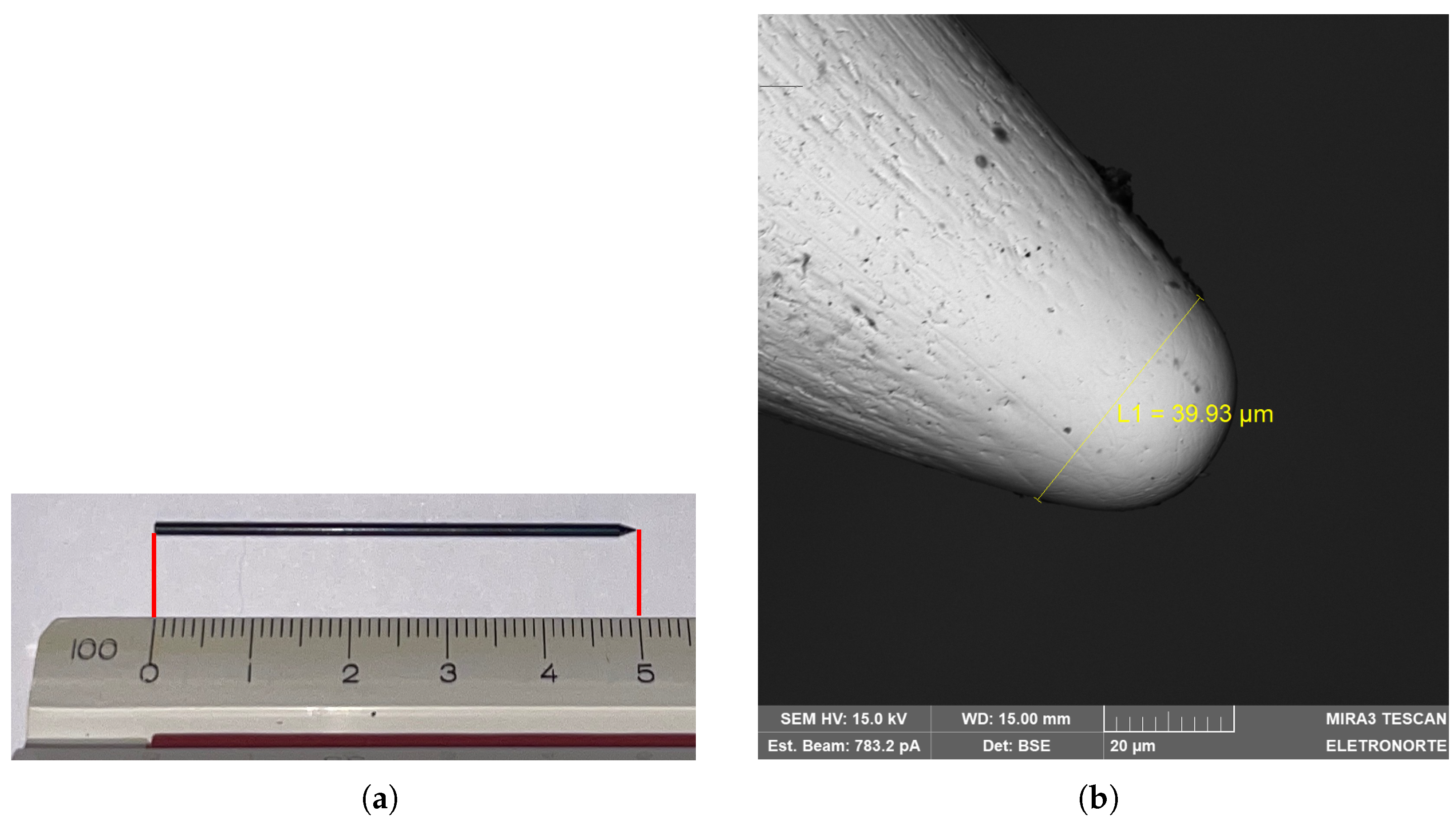
The conceived experimental setup is a point-plane configuration of electrodes at atmospheric pressure and subjected to a constant high voltage over time. The high voltage is applied to an Ogura X-253-7 steel needle, which is the same model used by Eichwald et al. in [3], and the ground plane is made of copper. The needle is a cylinder measuring 1 mm in diameter, and its tip is shaped like a cone (Figure 1a). 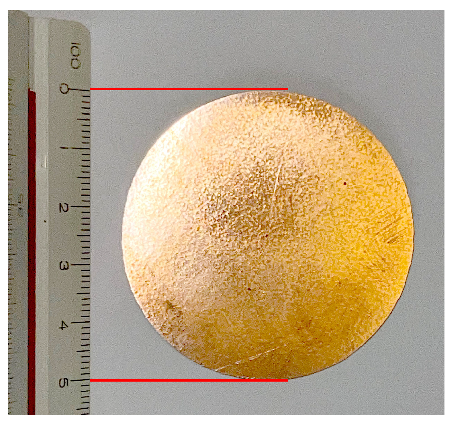The end of the needle consists of a sphere with radius of curvature of 20 $\mathsf{\mu }$m (Figure 1b). The copper plane is a disc with diameter of 5 cm, as shown in Figure 2, made from a blank FR4 PCB.

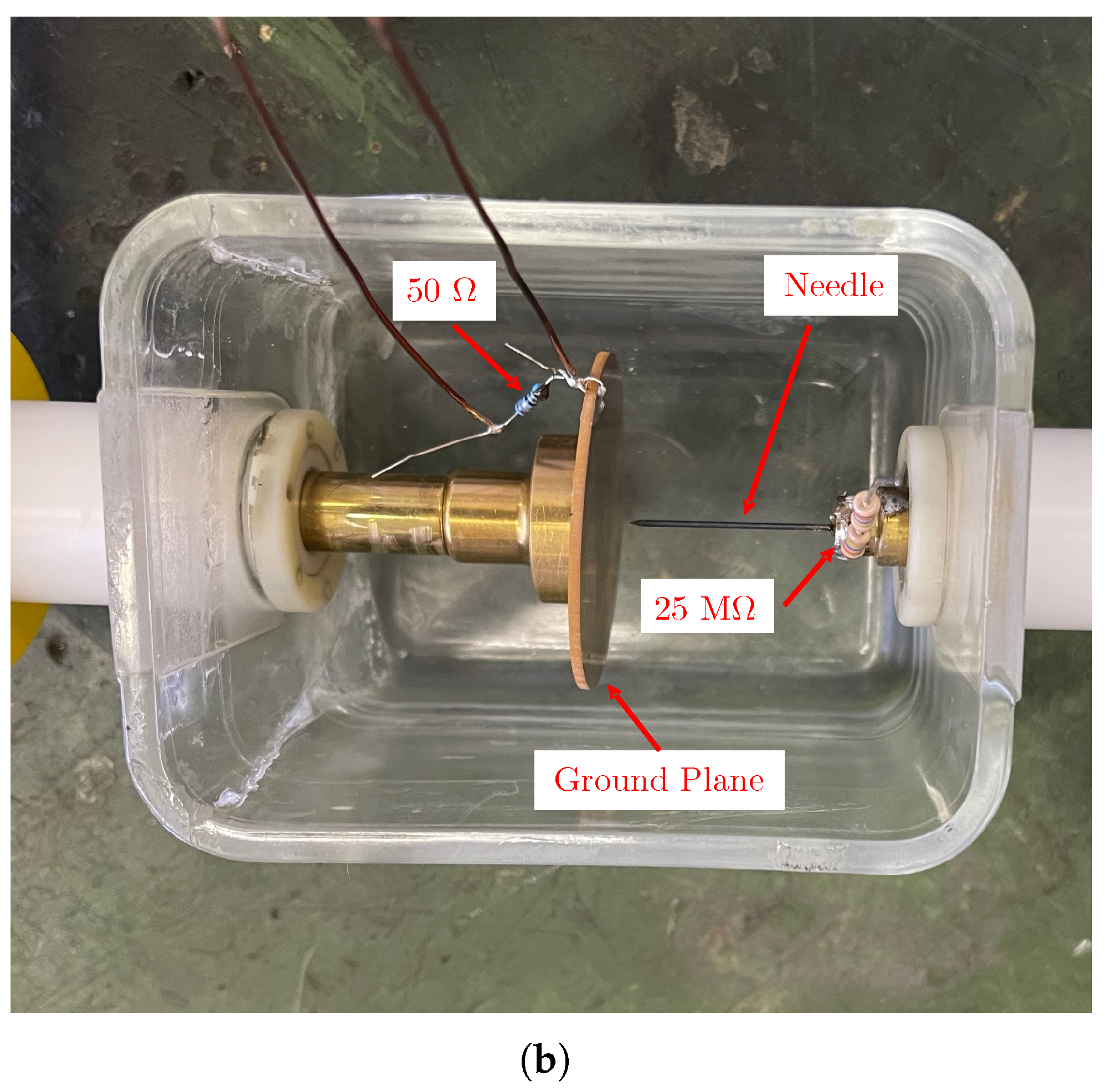
The experiments were conducted using two configurations: the first one in an environment where humidity was not controlled (Figure 3a) and the second one in an enclosed glass container used to control the air humidity (Figure 3b). To carry out the experiments, it was ensured that the needle was dry. To achieve this goal, the test room (with the measuring setup) was left closed with the air conditioner turned on for at least 12 h. During the experiments, air humidity was monitored using a digital table hygrometer.

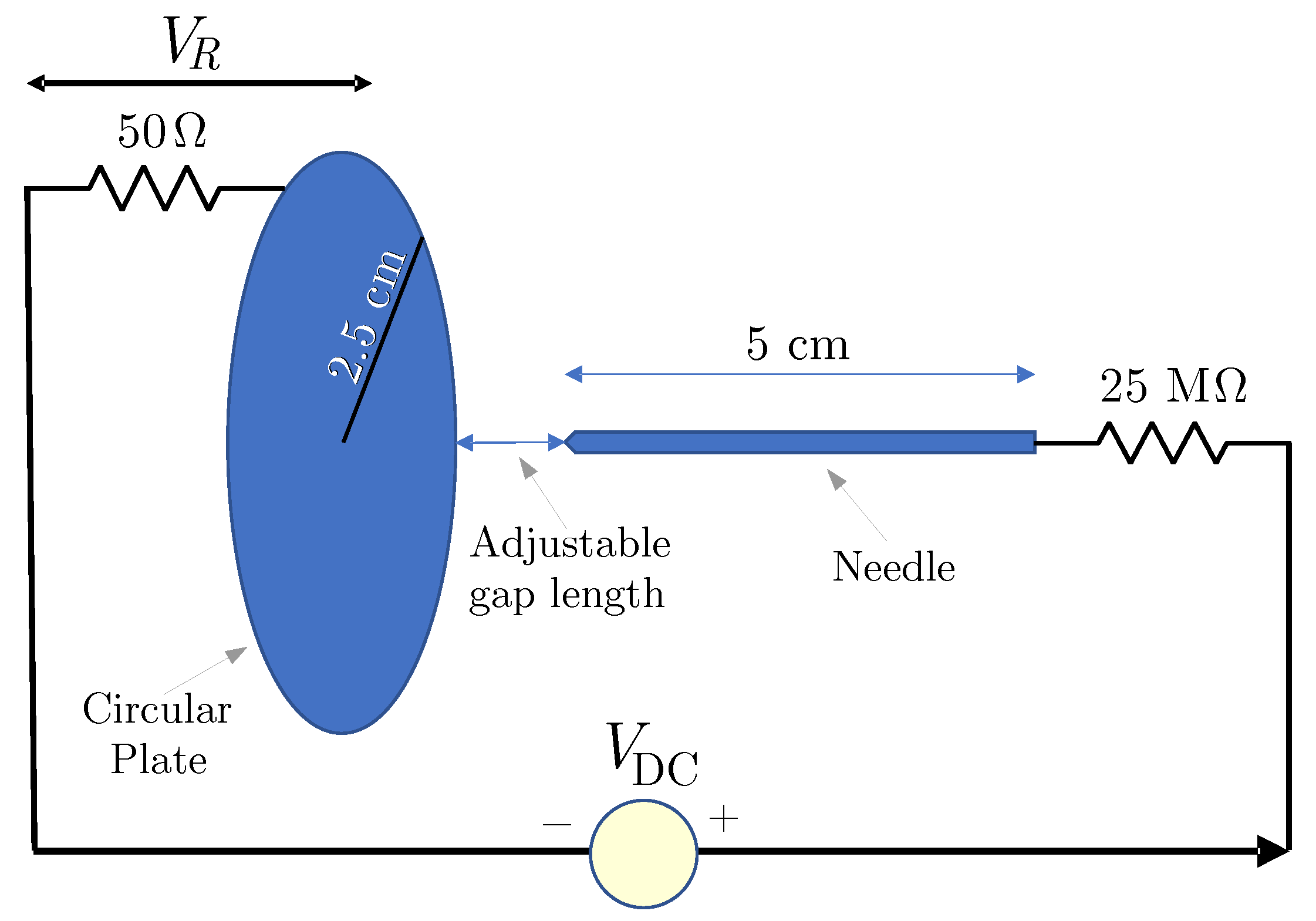
The discharge waveform is obtained by measuring the transient voltage across a 50 $\mathsf{\Omega }$ resistor, which can be seen in Figure 3. The current is limited using a 25 M$\mathsf{\Omega }$ resistor in order to prevent the triggering of the power supply’s over-current protection. Figure 4 shows the circuit schematics used for producing partial discharges and for measuring transient currents.

The experiments are conducted with gaps between the anode and the cathode of 4, 5, 6, 7, and 8 mm. Gap lengths are carefully adjusted using spacers obtained using a 3D printer (Figure 5). In the experiments, the voltage is gradually increased in such a way that the electric field surpasses the dielectric strength of air for each gap distance.

The breakdown voltage measured during the experiments for the 7 mm gap matched that obtained by Eichwald et al. in [3] (8.2 kV). In [3], current pulse measurements were conducted for the breakdown voltage $V_b=8.2$ kV and $0.878\times V_b=7.2$ kV. In our experiments, current waveform measurements were performed for voltages used in [3], as well as for other voltages selected above and below the breakdown voltage $V_b$ for each of the various gap distances, as systematically presented in

Table 1. Planned voltages to be applied and the obtained breakdown voltage $V_b$ for each gap length.

Gap Length (mm)	$0.878\times {\mathit{V}}_{\mathit{b}}$	$0.95\times {\mathit{V}}_{\mathit{b}}$	${\mathit{V}}_{\mathit{b}}$	$1.05\times {\mathit{V}}_{\mathit{b}}$	$1.122\times {\mathit{V}}_{\mathit{b}}$
8	7815	8455	8900	9345	10,013
7	7200	7790	8200	8610	9225
6	6498	7030	7400	7770	8325
5	5707	6175	6500	6825	7313
4	4851	5249	5525	5801	6216

. Due to limitations of our equipment, the voltage values we planned to apply using our voltage source are typically slightly different from the actually applied values, which accounts for the slight discrepancies seen between Table 1 and

Table 2. The applied DC voltages for the various gap lengths used in this work.

Gap Length (mm)	Applied DC Voltages (V)
4	4851
	5248
	5525
	5801
	6198
5	6025
	6178
	6510
	6816
	7314
6	6486
	7048
	7408
	7778
	8323
7	7180
	7820
	8200
	8600
8	7818
	8455
	8900
	9347

. To obtain the minimum voltage $V_b$ in which discharges emerge, we incrementally adjusted the applied voltage. For applying voltages smaller than $V_b$, once $V_b$ is achieved, applied voltages are reduced.

During breakdown experiments conducted to measure breakdown voltages, it was observed that the transient currents for any given configuration were inconsistent, i.e., non-repeatable after a few discharge occurrences, which was primarily attributed to the observed deterioration of the needle tip caused by several repeated breakdown discharges, as depicted in Figure 6.

To produce partial discharges, electrical current limitation imposed by the 25 M$\mathsf{\Omega }$ resistor, which has also been used in [13] for controllably assuming the function of a dielectric barrier, also played a crucial role in preventing severe damage to the needle, which was undamaged during the conduction of PD measurements. Subsequent tests revealed that using new needles and the 25 M$\mathsf{\Omega }$ resistor and repeating experiments resulted in expected PD outcomes, indicating that the degradation of needle tips due to repeated electric breakdown discharges was a significant factor, but it was necessary for obtaining the breakdown voltages. Consequently, attention was given to using needles devoid of deterioration for PD current measurements, ensuring consistency in experimental outcomes. Please note that the 50 $\mathsf{\Omega }$ resistor is used for PD current recording via transient voltage measurements. This procedure is adopted in [13].

3. The Proposed Air Ionization Model

The formation of plasma in the air region between the needle and the plate is governed by three fundamental stages: pre-ionization, ionization, and deionization. The ionization is further divided into the stages called prebreakdown streamer (PBS), subdivided into phases 1 and 2, and breakdown streamer (BS) [15]. In this work, all those stages are identified, respectively, by the values of the subscript p given in increasing order.

Pre-ionization ($p=0$) is the stage at which, in a given region, the electric field has not yet reached the critical field $E_c$, i.e., the air has not yet been ionized. In this stage, the electric conductivity $\sigma$ remains constant due to the non-ionizing intensity of the electric field caused by the excitation source, which is unable to release electrons from the air atoms. Therefore, during pre-ionization, the conductivity is

$${\sigma }_p\left(t\right)={\sigma }_0^T,$$

(1)

where ${\sigma }_0^T={10}^{-9}$ S/m is the initial conductivity of air [24].

All three stages of ionization are governed by

$${\sigma }_p\left(t\right)={\sigma }_{(p-1)}^T{e}^{\left(t-t_p\right)/{\tau }_p}.$$

(2)

In (2), p is the index of the ongoing ionization stage ($1\le p\le 3$), $t_p$ is the initial ionization time of stage p, ${\tau }_p$ is the time constant of stage p and ${\sigma }_{(p-1)}^T$ is the threshold conductivity of phase $p-1$, i.e., the last value of conductivity calculated in the phase $p-1$.

When $p=1$, the first phase of the prebreakdown streamer begins. The electric field exceeds the air critical field, the air breaks down, and the number of free electrons increases exponentially, thus starting the process of air ionization. Starting from a certain level of ionization, that is, with a specific amount of free charges, before the complete formation of the discharge channel, the rate of production of free charges decreases and, consequently, the current increases less sharply compared to the prebreakdown streamer 1 phase. This stage is phase 2 of the prebreakdown streamer (when $p=2$ in (2)), in which the ionization parameters are adjusted so that the increased rate of conductivity is lower than in the previous phase. Finally, when $p=3$, the third stage of ionization occurs: breakdown streamer. This phase is initiated when the discharge channel reaches the plate, and it is characterized by a higher increase rate of electrical conductivity than in the previously described phases. This effect happens because the ionized channel creates an electric connection between the high-voltage electrodes. During this phase, the discharge current pulse has its peak. The progressive increase in the channel diameter and the reduction in electron mobility are represented in this work through a progressive increase of the critical field during the breakdown streamer process, which follows the relationship proposed in [15], given by

$$E_c=E_{c1}+\left(\frac{t-t_p}{m_t}\right)(E_{c2}-E_{c1}),$$

(3)

where $E_{c1}$ is the initial critical field of air, $E_{c2}$ is the maximum critical field reached during the breakdown streamer, and $m_t$ is the parameter that determines the rate of change in the critical field over time.

The increase in the critical field, representing the progressive increase of channel diameter and the reduction of electron mobility, represented by (3), favors the beginning of the last stage: deionization, indexed by $p=4$. Electrons return to their orbits and conductivity decreases until the ionization process starts again. The decreasing electric conductivity during this stage is mathematically represented by

$${\sigma }_4\left(t\right)={\sigma }_d^T{e}^{-\left(t-t_d\right)/{\tau }_d},$$

(4)

where ${\sigma }_d^T$ is the last calculated value of conductivity in the breakdown streamer phase ($p=3$), ${\tau }_d$ is the deionization time constant, and $t_d$ is the initial deionization time.

Figure 7 illustrates all experimentally obtained phases in this work for the gap length of 8 mm and the applied voltage of 8 kV. The discharge current pulses occur periodically. It is observed that the higher the applied voltage, the higher the pulse repetition rate [25,26]. In this sense, the electrical conductivity of the channel in the experiments never returns to its initial value ${\sigma }_0$, and the ionization process restarts with a residual conductivity value that, consequently, changes the subsequent current. This means the pulses are not exactly equal for a given voltage level with a fixed gap length during the sequence of discharge pulses. On the other hand, in our computer model, this effect is considered by previously computing the time average of several pulses obtained from the experimental results to obtain the model ionization parameters.

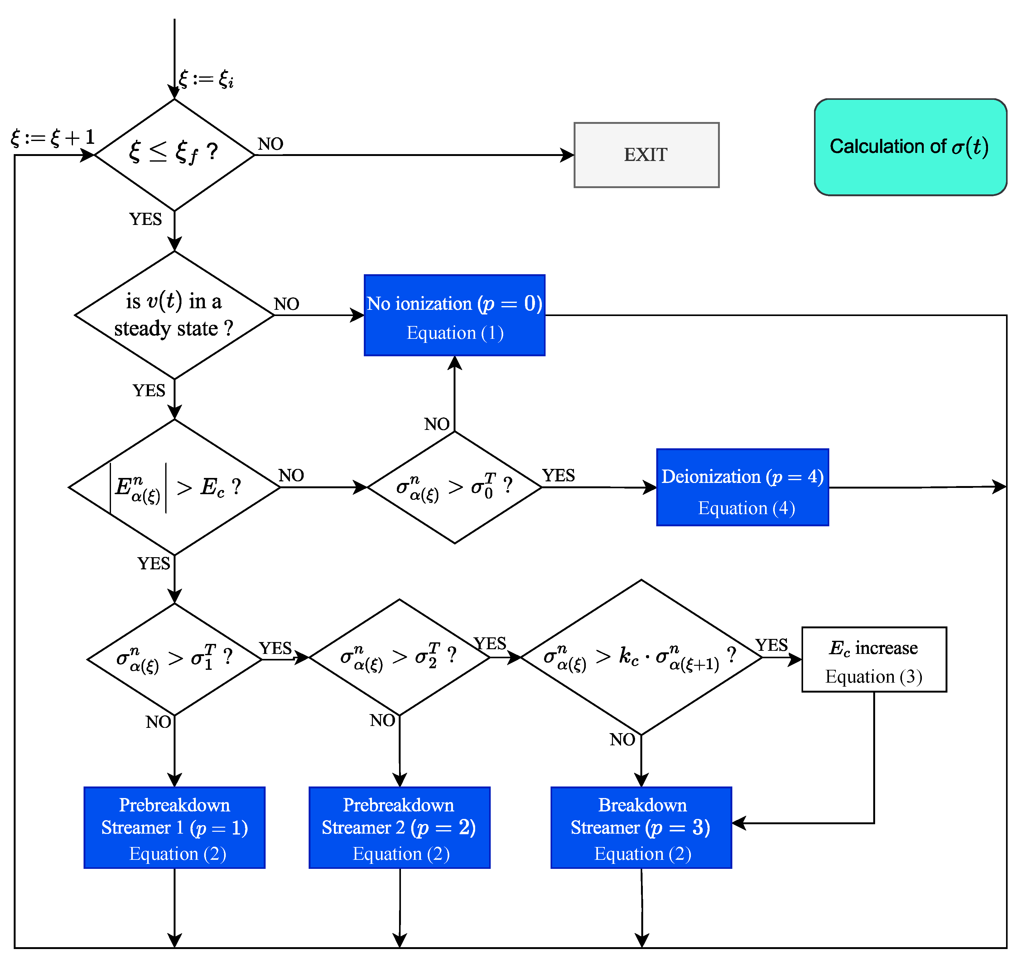
In Figure 8, the flowchart of the developed FDTD algorithm is shown. To include the proposed modeling of ionized air, the main differences with respect to the traditional FDTD algorithm are: defining the parameters of the ionization process; establishing the ionizable air path in which the discharge channel will be formed; and updating electrical conductivity $\sigma \left(t\right)$ in the temporal loop using (1)–(4).

In Figure 9, the procedure for updating electrical conductivity considering an ionizable path parallel to any Cartesian coordinate is presented in detail. Although electric field, magnetic field, and electrical conductivity are calculated throughout the three-dimensional domain, the ionizable path is considered to be one-dimensional in this work. The calculation of $\sigma$ is contained in a spatial loop over any line segment parallel to a Cartesian axis with index $\xi$, which may be i, j or k, indexing $\alpha$, which may be x, y and z, respectively. It is necessary to identify limits for $\xi$, where $\xi ={\xi }_i$ maps the first Yee cell of the ionizable path, and $\xi ={\xi }_f$ maps the last Yee cell on the ionizable path. Of course, the other two indexes regarding the other two Cartesian coordinates are set to be constant. The stages of the prebreakdown streamer ($p=1$ and $p=2$), breakdown streamer stage ($p=3$), and deionization stage ($p=4$) are represented by blue blocks properly identified.

In this work, the model described in [15] was adapted to DC voltage based on experimental results. In this sense, all key steps of the model presented in Figure 9 will only be carried out when the excitation source is in its DC steady-state regime, i.e., after the transient period emerging once the source is powered on.

The critical electric field $E_c$ is considered to be variable. Before starting the time loop, $E_c=E_{c1}$ is established as an initial critical field. As long as the strength of the electric field $|E_{\alpha \left(\xi \right)}^n|$ at a point in the ionizable path is smaller than the critical field $E_c$, the ionization process does not occur and, therefore, ${\sigma }_{\alpha \left(\xi \right)}^n$ remains equal to ${\sigma }_0^T$, i.e., the pre-ionization phase is ongoing [15].

When $|E_{\alpha \left(\xi \right)}^n|$ exceeds $E_c$, phase 1 of the prebreakdown streamer begins, i.e., the first air ionization stage takes place. At this state, the conductivity increases according to (2) with $p=1$ (parameters $t_1$, ${\tau }_1$ and ${\sigma }_0$ are used) while not exceeding the threshold defined here as ${\sigma }_1^T$. Once electric conductivity surpasses the ${\sigma }_1^T$ threshold, the increase rate of $\sigma$ is seen to be smaller than in the previous ionization stage, which persists up to the moment when the plasma channel is completely formed. This conductivity increase profile is modeled by phase 2 of the prebreakdown streamer, which is governed by (2) with $p=2$ ($t_2$, ${\tau }_2$ and ${\sigma }_1^T$ are the used parameters).

As soon as the conductivity at all points of the ionizable path becomes greater than the threshold ${\sigma }_2^T$, the plasma channel is considered to be fully formed, and then the conductivity begins to increase with its higher raise rate. This stage is modeled by the breakdown streamer phase, where $\sigma$ follows (2) with $p=3$ ($t_3$, ${\tau }_3$ and ${\sigma }_2^T$ are used). Still, at this stage, the augment of the critical field $E_c$ is modeled using the linear function described by (3). The intensification of $E_c$ is applied at a given point $\xi$ only when ${\sigma }_{\alpha \left(\xi \right)}$ is equal to or greater than the conductivity of the neighbor point immediately closest to the anode needle, i.e., when ${\sigma }_{\alpha \left(\xi \right)}\ge {\sigma }_{\alpha (\xi +1)}$.

As $\sigma$ increases, we observe, as a result of Maxwell’s equations, a consequent reduction of electric field strength at the discharge channel points. The deionization phase occurs when $|E_{\alpha \left(\xi \right)}^n|$ reduces to a level where $\left|E_{\alpha \left(\xi \right)}^n\right|\le E_c$ and, at this stage, the conductivity decreases as described by (4). In [15], ${\tau }_d$ was modeled by a decreasing sigmoid to represent with good accuracy the interaction process between the charges present in the channel. However, in the present model, which has been adapted to the DC voltage regime, it was not necessary. Therefore, ${\tau }_d$ assumes a constant value for each applied ionizing voltage.

4. Results and Discussion

The constants in (2) and (4) were obtained by estimating the rise and decay times for each phase of ionization and deionization. In this sense, for each voltage level and gap length, optimal values were estimated for reproducing the experimental electric currents obtained in this work. Table 2 shows the obtained values of all parameters for each studied voltage level and gap length. It is important to emphasize that ${\tau }_1=3.8$ ns, $E_{c1}=10$ kV/m, $E_{c2}=4$ MV/m and $k_c=1.01$ were used for all numerical simulations. 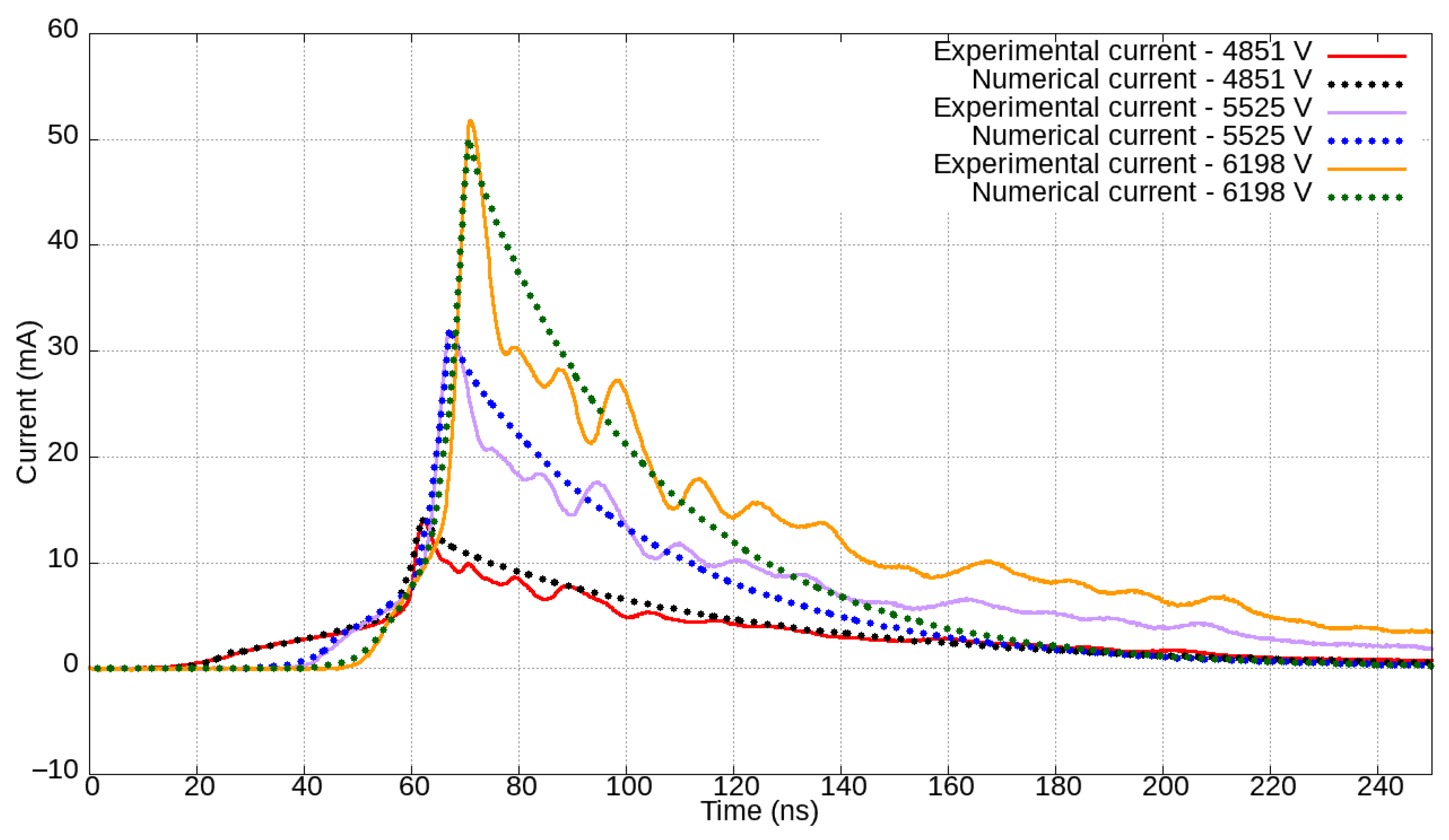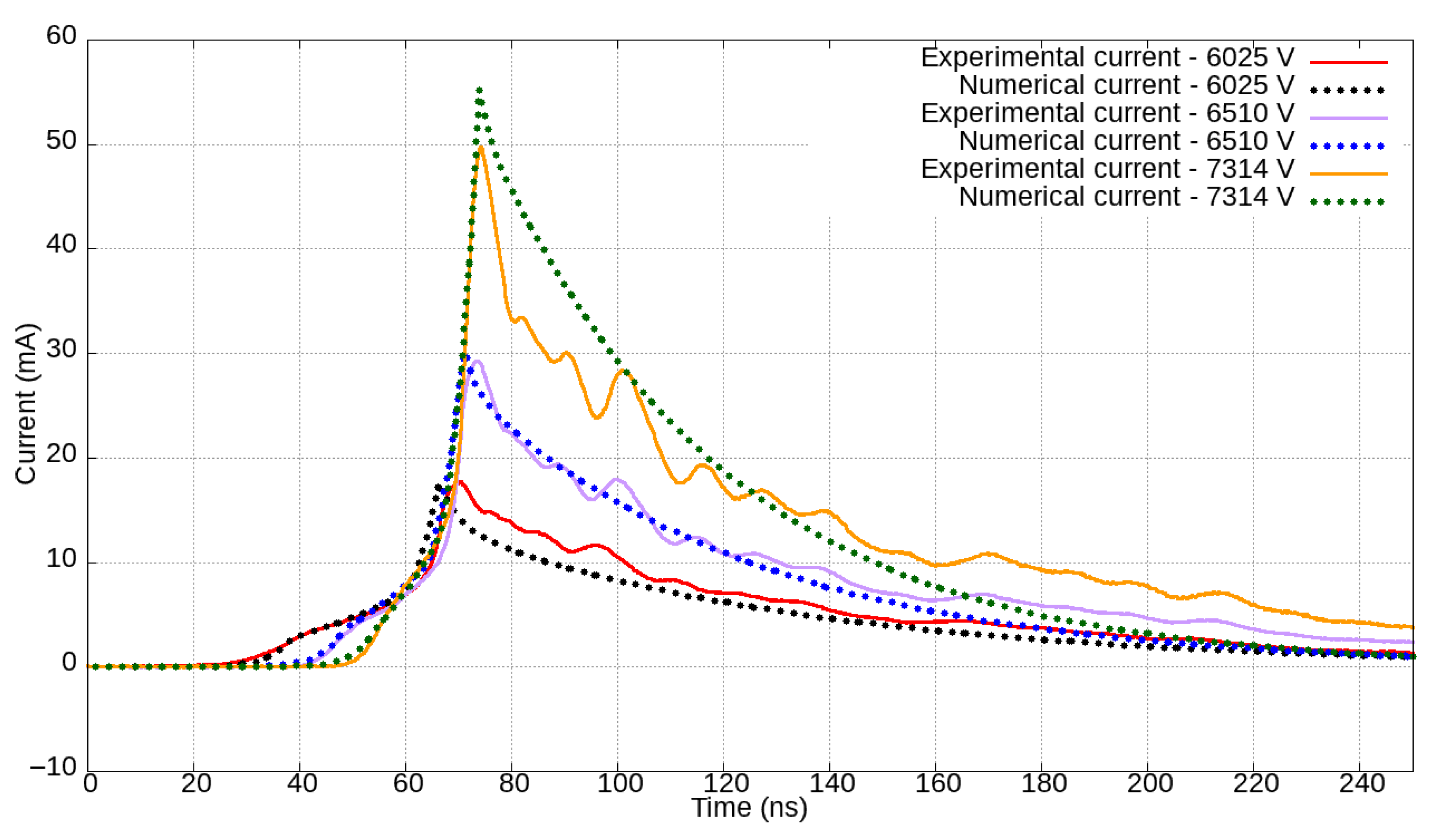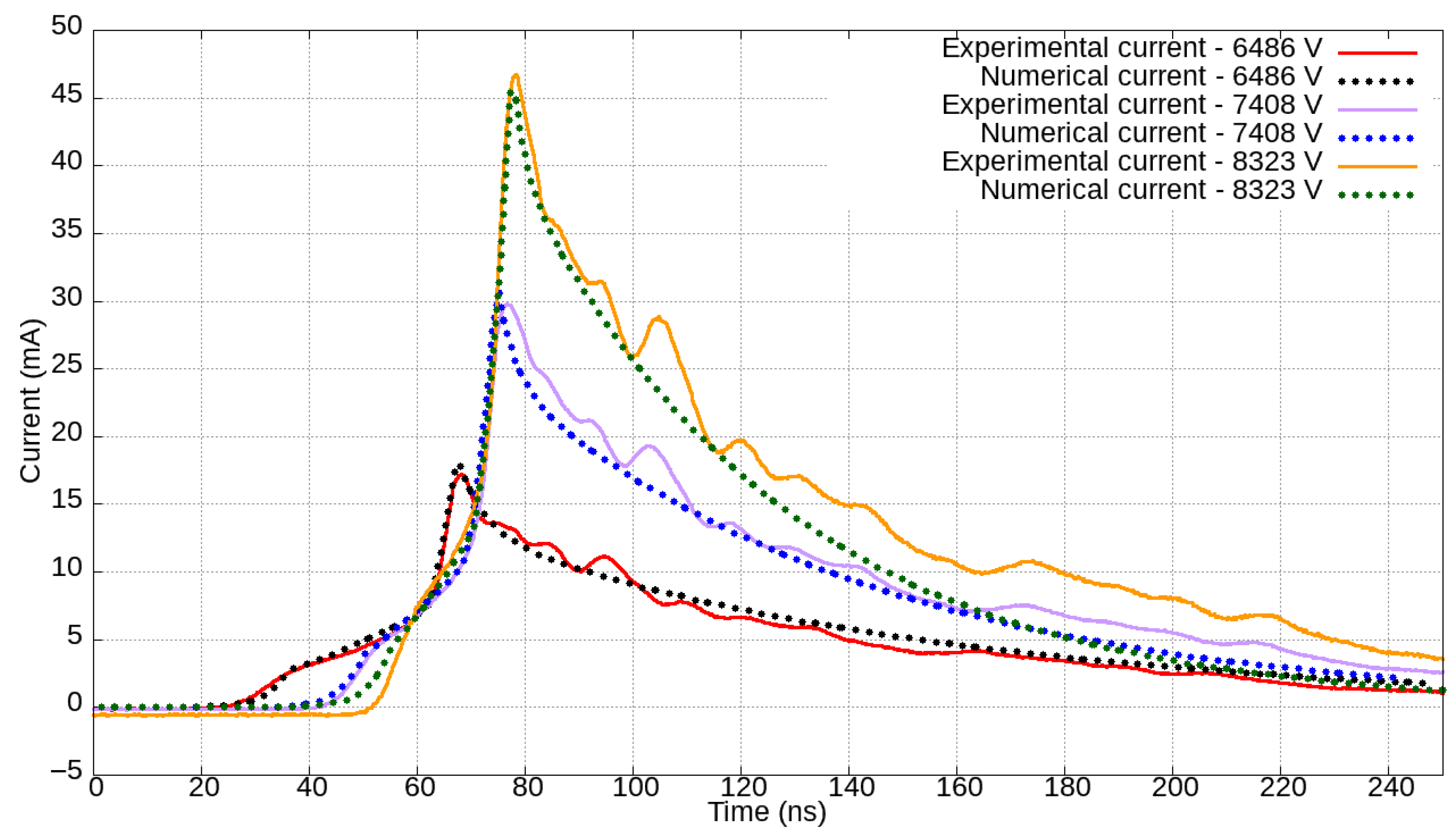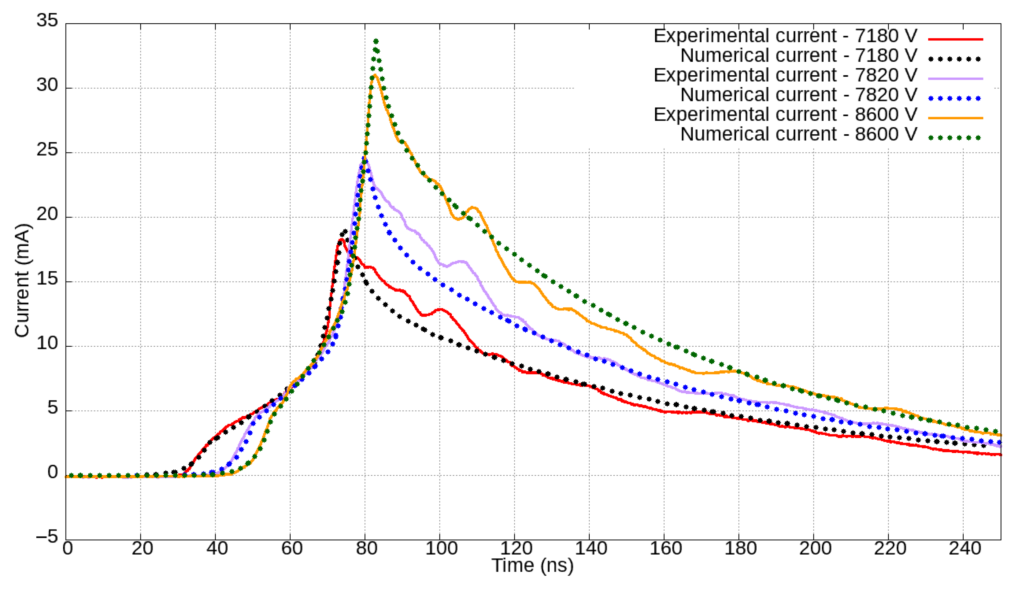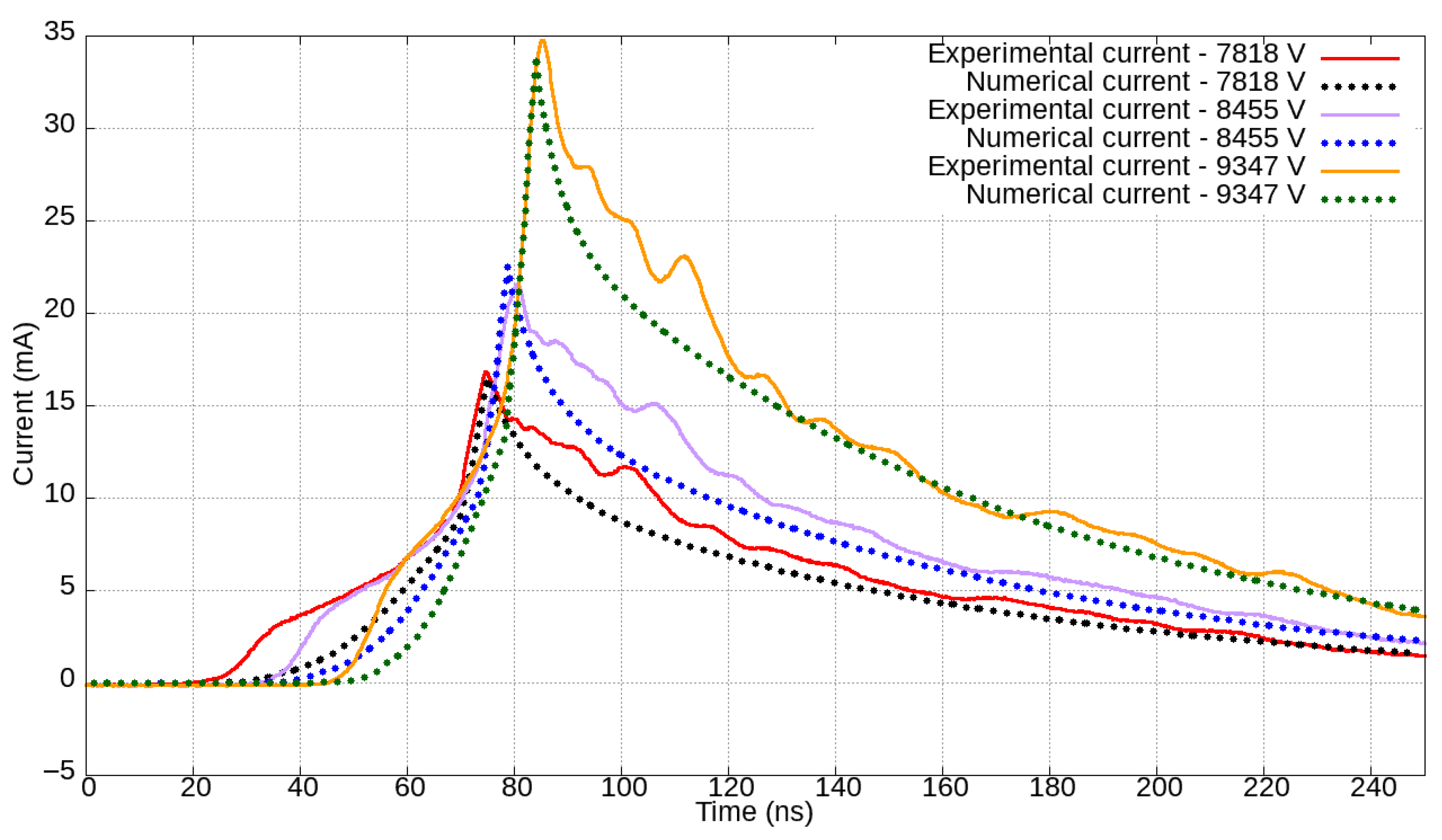Figure 10, Figure 11, Figure 12, Figure 13 and Figure 14 show the experimental and calculated electric currents for gaps of 4, 5, 6, 7, and 8 mm, respectively, for respective applied voltage levels.

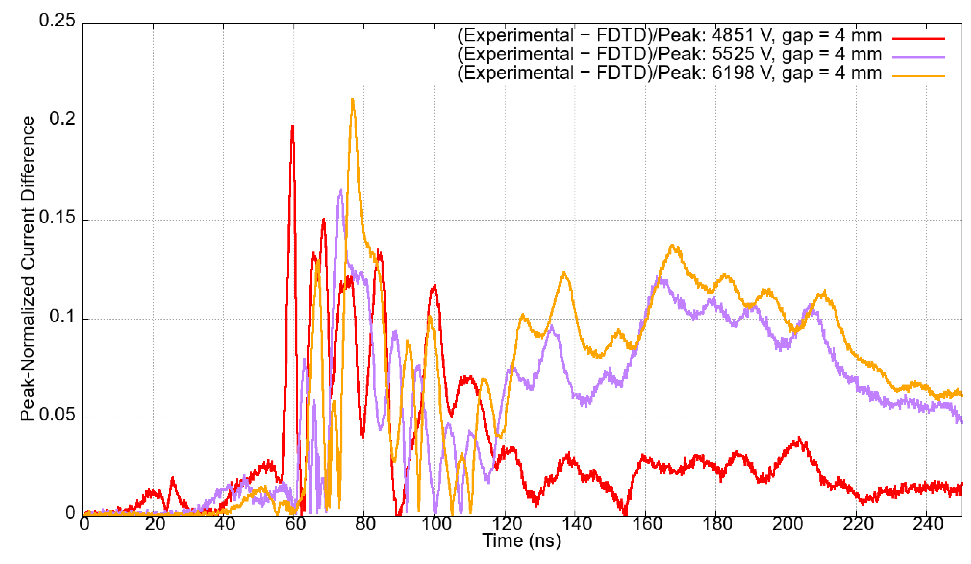
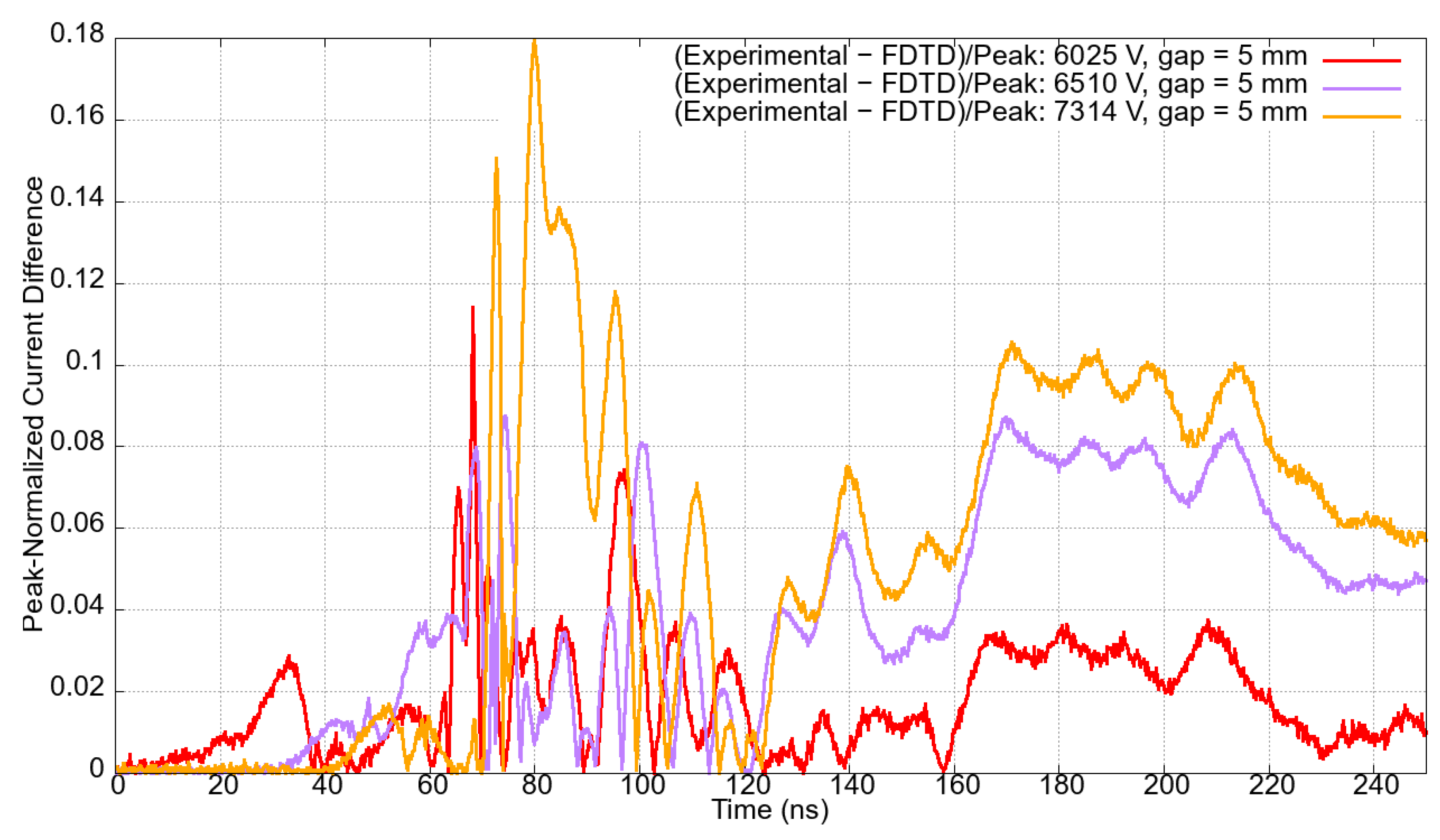
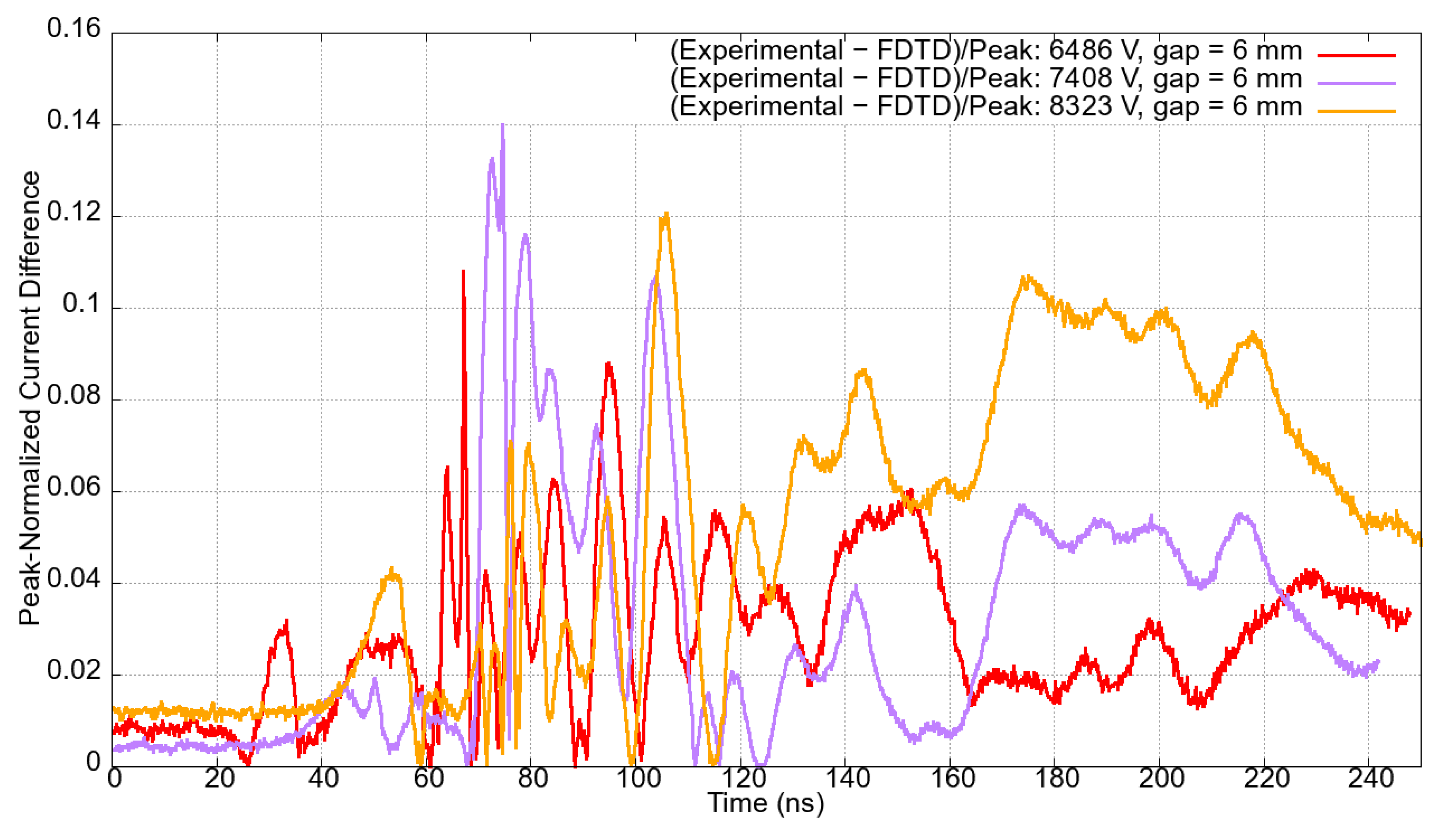
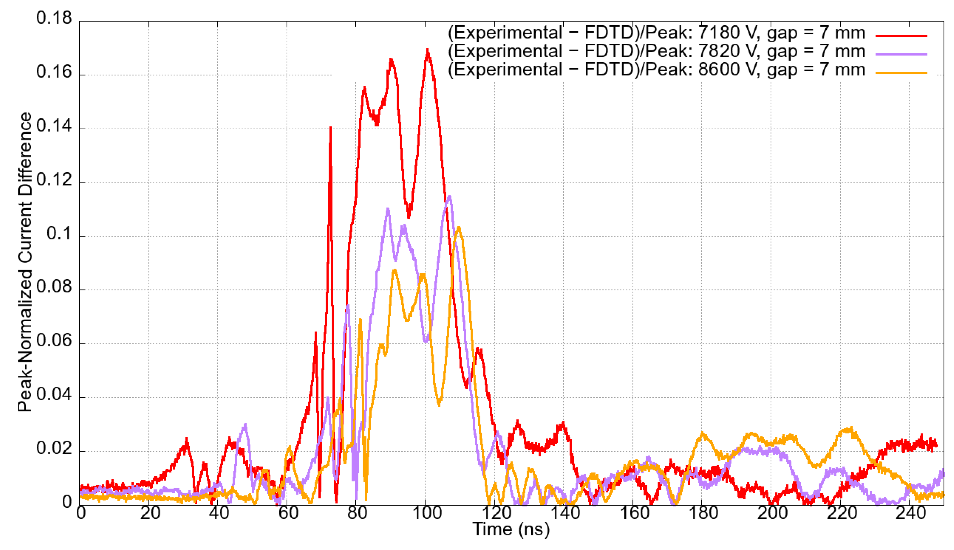
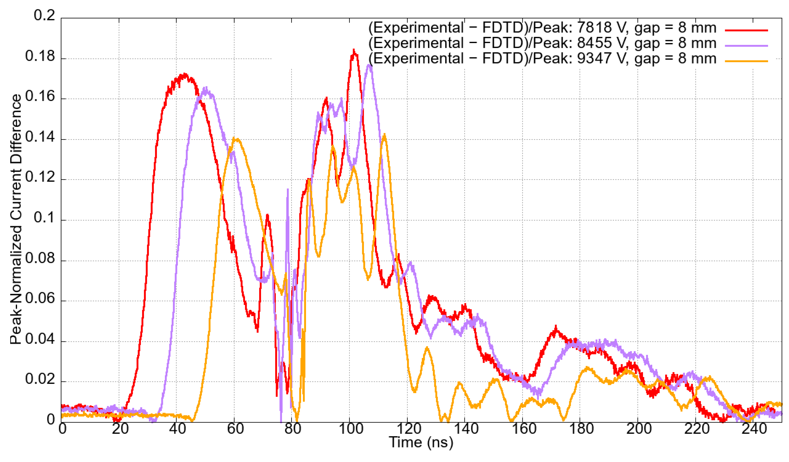
Absolute peak-normalized errors between experimental and simulation currents over time, given in Figure 10, Figure 11, Figure 12, Figure 13 and Figure 14, have been calculated. Figure 15, Figure 16, Figure 17, Figure 18 and Figure 19 display graphs illustrating peak-normalized differences, over time, between the experimental and numerical data for each gap length and their corresponding applied voltages. Notably, the peak-normalized current differences consistently remain below 0.20 for most of the time and across all the various experiments. The difference reached 0.20 solely to the case with a gap length of 4 mm excited by voltages 4851 V and 6198 V. The smallest maximum deviation slightly above 0.1 is seen for the case in which the gap length measures 7 mm, and the excitation voltage is 8.6 kV.

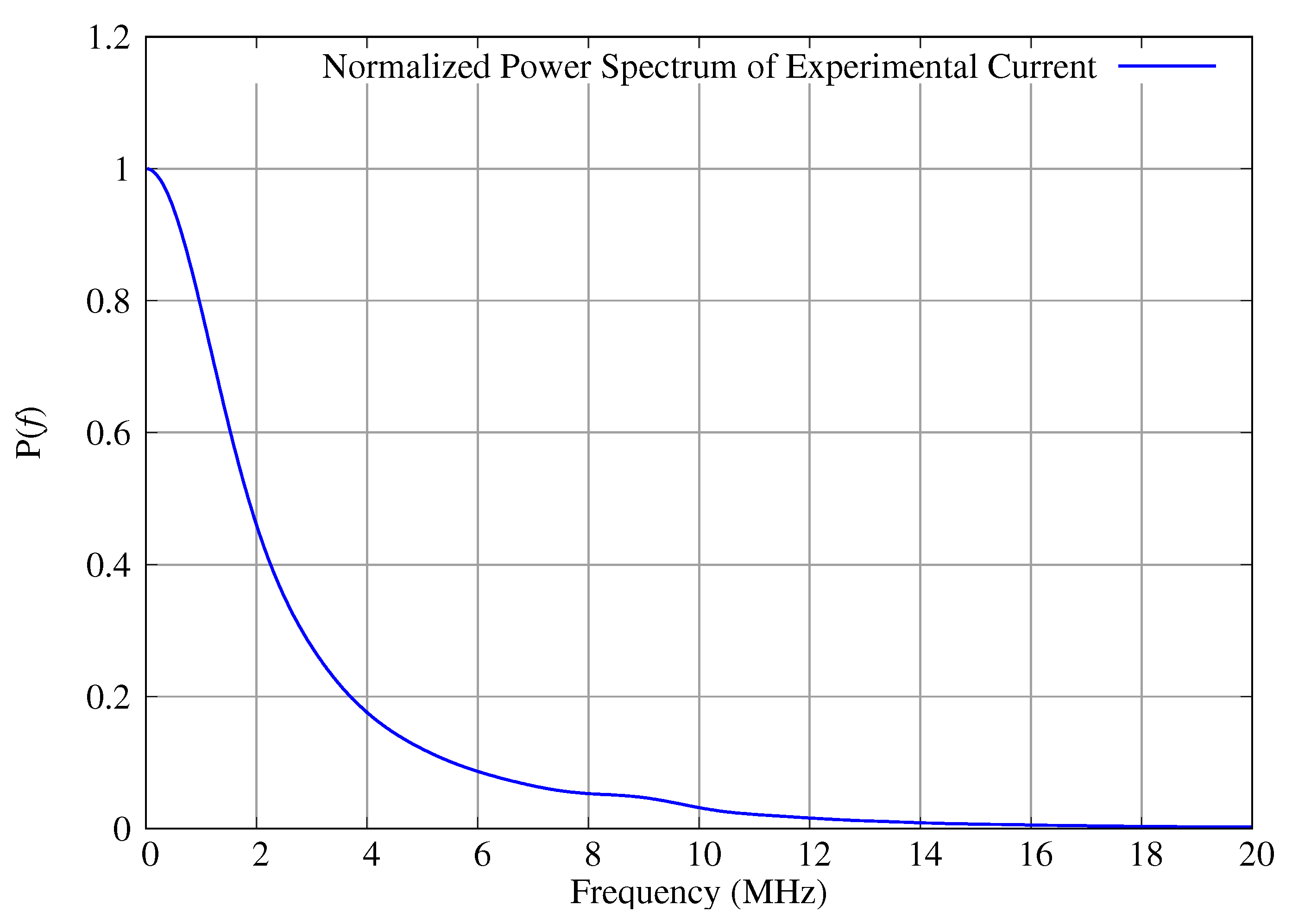
In our FDTD implementation, the thin wire model by Y. Taniguchi and Y. Baba et al. [27] was employed for representing the conducting wires. The circuit conductor dimensions (lengths and diameters of approximately 0.1 m and 1.13 mm, respectively, reproducing the experimental conditions) are much smaller than the minimum wavelength ${\lambda }_{\min }\approx 20$ m, as the maximum frequency of significant power of current pulses is about 15 MHz (see Figure 20), indicating that we have a lumped circuit. Conductor resistance is much smaller than plasma channel resistance since the conductivity of copper is about eight orders of magnitude over the maximum conductivity of ionized air. Nevertheless, copper wire resistance and inductance have both been accounted for in the FDTD model using the thin wire formulation. The FDTD spatial domain has been truncated using Gedney’s uniaxial perfectly matched layer formulation (UPML) [28].

The constant ${\tau }_1$ depends solely on the geometry of the needle tip and on the parameters of the gas being ionized. In this regard, ionization will initially occur independently of the gap length, as the electric field emerging in the vicinity of the needle tip is determinant for defining the profile of the electronic dissociation of the first atoms ionized. Therefore, ${\tau }_1$ defines the initial increase rate of conductivity, which is observed to be constant for all experiments carried out in this work.

The closer the electrodes are, the greater the variation of ionization parameters as functions of voltage level (see

Table 3. The model parameters estimated for each gap length and voltage level. The given parameters were used in FDTD simulations.

Gap Length (mm)	Applied Voltages (V)	${\mathit{\tau }}_2$ (s)	${\mathit{\tau }}_3$ (s)	${\mathit{\tau }}_{\mathit{d}}$ (s)	${\mathit{\sigma }}_1^{\mathit{T}}$ (S/m)	${\mathit{\sigma }}_2^{\mathit{T}}$ (S/m)	${\mathit{m}}_{\mathit{t}}$ (s)
4	4851	$1.3\times {10}^{-8}$	$4.0\times {10}^{-9}$	$6.0\times {10}^{-8}$	$1.0\times {10}^{-3}$	$1.1\times {10}^{-2}$	$1.39\times {10}^{-8}$
	5248	$1.0\times {10}^{-8}$	$3.5\times {10}^{-9}$	$4.7\times {10}^{-8}$	$1.0\times {10}^{-3}$	$1.1\times {10}^{-2}$	$1.39\times {10}^{-8}$
	5525	$0.8\times {10}^{-8}$	$3.3\times {10}^{-9}$	$4.0\times {10}^{-8}$	$2.0\times {10}^{-3}$	$1.2\times {10}^{-2}$	$1.7\times {10}^{-8}$
	5801	$0.6\times {10}^{-8}$	$3.1\times {10}^{-9}$	$3.5\times {10}^{-8}$	$2.0\times {10}^{-3}$	$1.2\times {10}^{-2}$	$1.7\times {10}^{-8}$
	6198	$0.5\times {10}^{-8}$	$3.0\times {10}^{-9}$	$3.5\times {10}^{-8}$	$2.0\times {10}^{-3}$	$1.2\times {10}^{-2}$	$1.7\times {10}^{-8}$
5	6025	$1.1\times {10}^{-8}$	$4.5\times {10}^{-9}$	$7.0\times {10}^{-8}$	$1.6\times {10}^{-3}$	$1.2\times {10}^{-2}$	$1.39\times {10}^{-8}$
	6178	$0.9\times {10}^{-8}$	$4.1\times {10}^{-9}$	$6.0\times {10}^{-8}$	$2.0\times {10}^{-3}$	$1.5\times {10}^{-2}$	$1.7\times {10}^{-8}$
	6510	$0.8\times {10}^{-8}$	$4.0\times {10}^{-9}$	$5.5\times {10}^{-8}$	$2.0\times {10}^{-3}$	$1.5\times {10}^{-2}$	$1.7\times {10}^{-8}$
	6816	$0.7\times {10}^{-8}$	$3.65\times {10}^{-9}$	$5.0\times {10}^{-8}$	$2.0\times {10}^{-3}$	$1.5\times {10}^{-2}$	$1.7\times {10}^{-8}$
	7314	$0.6\times {10}^{-8}$	$3.12\times {10}^{-9}$	$4.5\times {10}^{-8}$	$2.0\times {10}^{-3}$	$1.5\times {10}^{-2}$	$1.7\times {10}^{-8}$
6	6486	$1.2\times {10}^{-8}$	$4.2\times {10}^{-9}$	$9.0\times {10}^{-8}$	$1.5\times {10}^{-3}$	$1.3\times {10}^{-2}$	$1.3\times {10}^{-8}$
	7048	$0.95\times {10}^{-8}$	$4.0\times {10}^{-9}$	$8.5\times {10}^{-8}$	$1.5\times {10}^{-3}$	$1.3\times {10}^{-2}$	$1.45\times {10}^{-8}$
	7408	$0.9\times {10}^{-8}$	$3.8\times {10}^{-9}$	$6.9\times {10}^{-8}$	$2.0\times {10}^{-3}$	$1.6\times {10}^{-2}$	$1.4\times {10}^{-8}$
	7778	$0.8\times {10}^{-8}$	$3.7\times {10}^{-9}$	$5.9\times {10}^{-8}$	$2.0\times {10}^{-3}$	$1.6\times {10}^{-2}$	$1.55\times {10}^{-8}$
	8323	$0.74\times {10}^{-8}$	$3.6\times {10}^{-9}$	$5.0\times {10}^{-8}$	$2.0\times {10}^{-3}$	$1.6\times {10}^{-2}$	$1.61\times {10}^{-8}$
7	7180	$1.15\times {10}^{-8}$	$6.8\times {10}^{-9}$	$9.0\times {10}^{-8}$	$1.3\times {10}^{-3}$	$1.6\times {10}^{-2}$	$1.85\times {10}^{-8}$
	7820	$1.05\times {10}^{-8}$	$5.6\times {10}^{-9}$	$8.5\times {10}^{-8}$	$2.0\times {10}^{-3}$	$1.6\times {10}^{-2}$	$1.9\times {10}^{-8}$
	8200	$0.9\times {10}^{-8}$	$5.5\times {10}^{-9}$	$8.0\times {10}^{-8}$	$2.0\times {10}^{-3}$	$1.9\times {10}^{-2}$	$1.9\times {10}^{-8}$
	8600	$0.88\times {10}^{-8}$	$5.2\times {10}^{-9}$	$8.0\times {10}^{-8}$	$2.0\times {10}^{-3}$	$1.9\times {10}^{-2}$	$1.9\times {10}^{-8}$
8	7818	$1.35\times {10}^{-8}$	$5.5\times {10}^{-9}$	$9.0\times {10}^{-8}$	$1.5\times {10}^{-3}$	$1.9\times {10}^{-2}$	$1.2\times {10}^{-8}$
	8455	$1.19\times {10}^{-8}$	$5.0\times {10}^{-9}$	$9.0\times {10}^{-8}$	$1.5\times {10}^{-3}$	$1.9\times {10}^{-2}$	$1.2\times {10}^{-8}$
	8900	$1.13\times {10}^{-8}$	$4.5\times {10}^{-9}$	$9.0\times {10}^{-8}$	$2.4\times {10}^{-3}$	$2.2\times {10}^{-2}$	$1.28\times {10}^{-8}$
	9347	$1.0\times {10}^{-8}$	$4.5\times {10}^{-9}$	$9.0\times {10}^{-8}$	$2.4\times {10}^{-3}$	$2.2\times {10}^{-2}$	$1.3\times {10}^{-8}$

). This is seen especially for ${\tau }_2$, ${\tau }_3$, ${\tau }_d$ and $m_t$.

The constant ${\tau }_2$ is also strongly influenced by the source voltage level. As the voltage level increases, ${\tau }_2$ reduces accordingly, as one would expect, since electrons experience acceleration augmentation as the intensity of the electric field increases. Likewise, ${\tau }_3$ also decreases with increasing voltage, for the same reason, favoring current peak increase with voltage during phase 3. Please note that ${\tau }_3$ is one order of magnitude smaller than ${\tau }_2$ because of the electric connection established between the high-voltage electrodes through the ionized channel. Electrons gain additional acceleration due to the high voltage set between the ends of the channel.

According to Table 3, ${\tau }_d$ also decreases with increasing voltage. The smaller ${\tau }_d$ is, the faster the deionization process. It can be seen that the greater the distance between the electrodes, the greater ${\tau }_d$ is, i.e., the deionization process will be slower when compared to smaller gaps (see Table 3). Thus, deionization time decreases with both increasing voltage and decreasing gap length. This is because stronger repulsion forces among electric charges arise due to both changes, favoring reassociation [25,26].

The parameters ${\sigma }_1^T$, ${\sigma }_2^T$, and $m_t$ define the duration of the ionization phases. Higher voltage leads to increased values of ${\sigma }_1^T$, as shown in Table 3. However, this increase in ${\sigma }_1^T$ becomes less pronounced as the gap spacing between the electrodes widens. Similar behavior is seen in parameters ${\sigma }_2^T$ and $m_t$, which also tend to saturate (reach a constant value) with increasing voltage.

The critical electric field $E_{c1}$ is the minimum electric field at which ionization occurs. This parameter depends solely on the dimensions of the needle tip, the applied voltage level, and the characteristics of the gas. The cathode is not influential in this initial stage. Therefore, $E_{c1}$ does not depend on the gap length and, consequently, remains constant across all simulations. In (3), the critical electric field $E_{c2}$ is also considered to be constant. Therefore, since current follows Ohm’s law $\overrightarrow{J}=\sigma ·\overrightarrow{E}$, the parameters determining the peak current are ${\sigma }_2^T$ and the voltage level, along with gap size.

The parameter $k_c$ is an algorithmic constant introduced to enable proper differentiation of electrical conductivities between neighbor FDTD cells in the gap discharge channel (see Figure 9). This is necessary to enable the independent evolution of conductivities across all Yee cells in the gap for the specific case in which the ionization process occurs in a DC excitation voltage regime. To address this limitation, the algorithm proposed in [15] for transitory voltage excitation is adopted in this work by incorporating $k_c=1.01$, as detailed in Figure 9. This parameter remains constant across all numerical simulations. For the sake of comparison, the algorithm proposed in [15] could have been implemented with the algorithm of this paper with $k_c=1$.

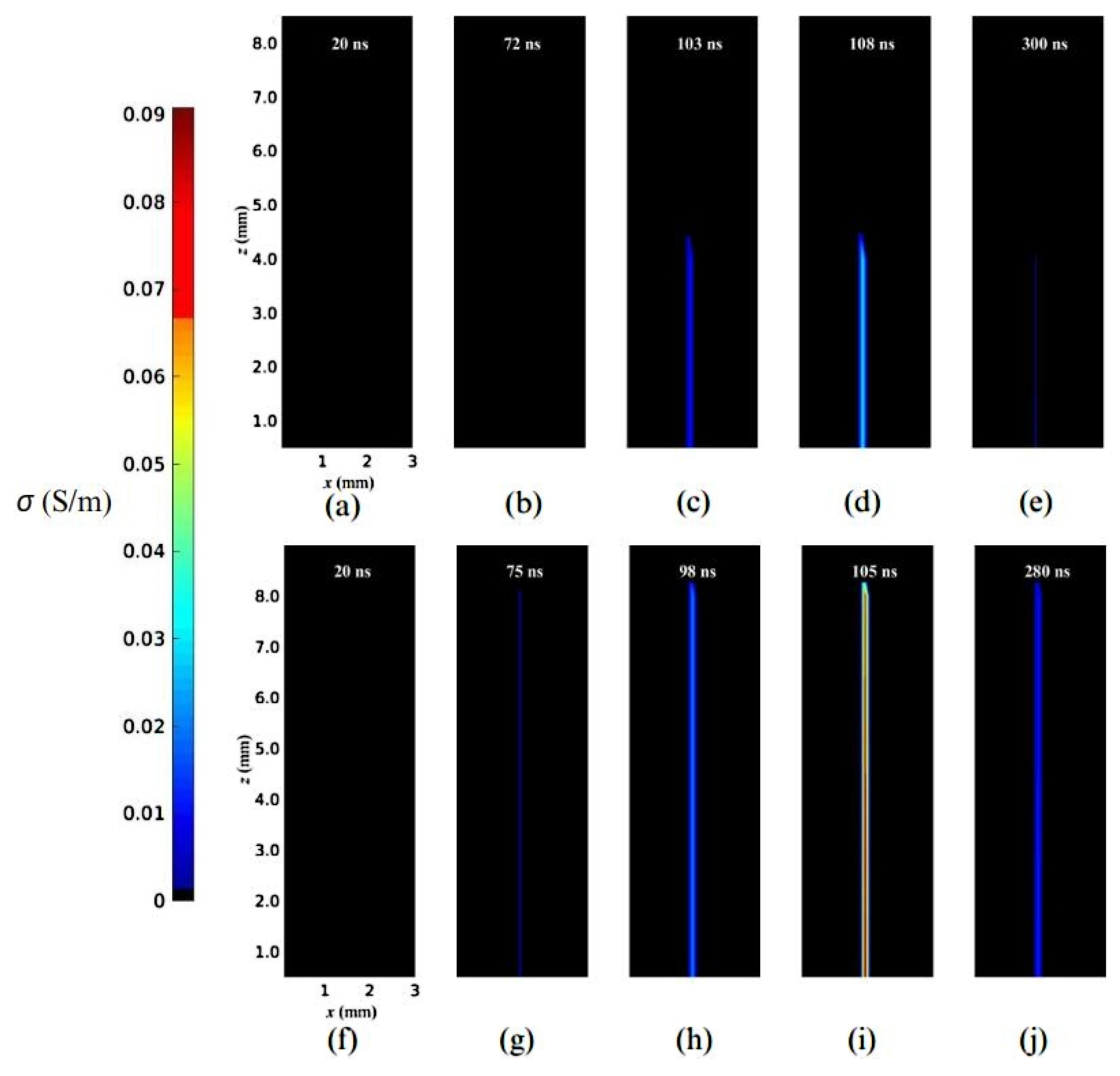
Figure 21 illustrates the temporal and spatial evolution of $\sigma$ for gap lengths measuring 4 mm and 8 mm. Figure 21a and Figure 21f depict the preionization-phase conductivity for voltages of 4851 V and 9347 V, respectively. The prebreakdown streamer 1 phase has the channel conductivity represented in Figure 21b,g. Figure 21c,h were produced during the prebreakdown streamer 2 phase. The breakdown streamer phases for both gap lengths are illustrated in Figure 21d and Figure 21i, respectively. Finally, the conductivity in the deionization phase is depicted in Figure 21e,j.

In order to facilitate computer implementation, all optimal ionization parameters obtained in this work have been represented as functions via polynomial interpolation. Each parameter is given as a function of gap size and DC excitation voltage level v. The coefficients of the obtained polynomials are provided in Appendix A.

Regarding the computational aspects of our work, the FDTD model required VRAM usage of 392 MB and needed approximately 9 min to process each simulation. The employed FDTD mesh has 65 cells for each line parallel to each Cartesian axis (total of ${65}^3$ = 274,625 cells). We employed an NVIDIA GeForce RTX 3060 graphics card, utilizing all the available cores from the 3584 processing units. Notice that computational resources necessary for executing FDTD simulations are strongly linked to the total number of mesh cells: if geometric complexity is implemented for cases in which no requirements of a substantial increase of the number of cells are present, required computational resources would be similar to those used in this work; however, if the number of cells is duplicated for each Cartesian axis, memory requirements would be 8 times ($2^3$) that originally required.

5. Conclusions

In this study, we devised a formulation to model ionized air plasma conductivity of the needle-plate problem excited by DC high voltage utilizing the Finite-Difference Time-Domain (FDTD) method. The proposed model is rooted in results obtained from laboratory experiments and in the nonlinear manipulation of the electrical conductivity inherent in Maxwell’s equations in the proposed numerical model.

Within our proposed model, the electrical conductivity $\sigma$ undergoes temporal evolution and is computed for distinct ionization stages, encompassing phases 1 and 2 of the prebreakdown streamer, breakdown streamer, and deionization. The computation of $\sigma$, used in the Maxwell–Ampére equation within the FDTD method for updating the electric field over time, is executed via time-adapted functions sourced from relevant literature for each ionization stage.

Hence, we introduce formulas and general procedures suitable for numerically representing the ionized filament. Addressing the substantial impact of the gap distance involves identifying the moment when the streamer head reaches the anode plate, triggering the breakdown of the streamer phase. These constitute the primary contributions of this research.

The electromagnetic coupling between circuit components, including the ionized channel, needle, plate, and conducting wires, is properly represented by solving Maxwell’s equations using the FDTD method. Consequently, modifying the geometric features of the problem does not present a limitation in the formulation.

Validation of the proposed model in this study involved numerical-experimental comparisons of the tip-plane system response to voltages ranging from 4 kV to 9 kV and gap distances between 4 mm and 8 mm. The results demonstrated excellent agreement between the numerical data derived in this study and experimental observations. The maximum percentage deviation of the peak current, for instance, was 10.33% for the 7 mm gap length and 7180 V voltage case. On the other hand, the minimum deviation was 0.29% for the 7 mm gap length and 8600 V voltage case.

Experiments conducted as part of this research, the outcomes of which may be employed in future endeavors to extend the FDTD formulation introduced here, aim to present a more comprehensive representation of plasma channel conductivity across various parameters (voltage and gap distance). Factors such as rise times, decay times, and current peaks undoubtedly play fundamental roles in developing new mathematical formulations. Additionally, metrics such as photon counting, repetition rates, and the interdependence of discharge characteristics offer a broader understanding of the problem’s physics and hold promise in formulating new mathematical (numerical) models in the future. Finally, the FDTD method captures the dynamics of the plasma’s electrical conductivity evolution over time, considering the influence of applied DC voltage and gap length. This level of detail enables a comprehensive analysis of the spatiotemporal behavior of the plasma electromagnetic influence, which is essential for understanding and predicting the coupled phenomena under various conditions. In future works, realistic PD sources can be used in complex FDTD models of high-voltage devices to calculate their corresponding electromagnetic responses. Please note that we only considered sea-level atmospheric pressure in our study. A closed glass enclosure with an acrylic cover was used during the experiments, maintaining air with approximately 2% relative humidity and a temperature of 20 °C. Both humidity and temperature levels were kept constant throughout the experiments and in the development of the FDTD formulation process. The influence of environmental factors and different types of voltage excitation (AC or transient voltage regimes) can also be considered in future works.