
A Systematic Approach of Global Sensitivity Analysis and Its Application to a Model for the Quantification of Resilience of Interconnected Critical Infrastructures


Abstract
:1. Introduction
2. Modeling for Resilience Analysis
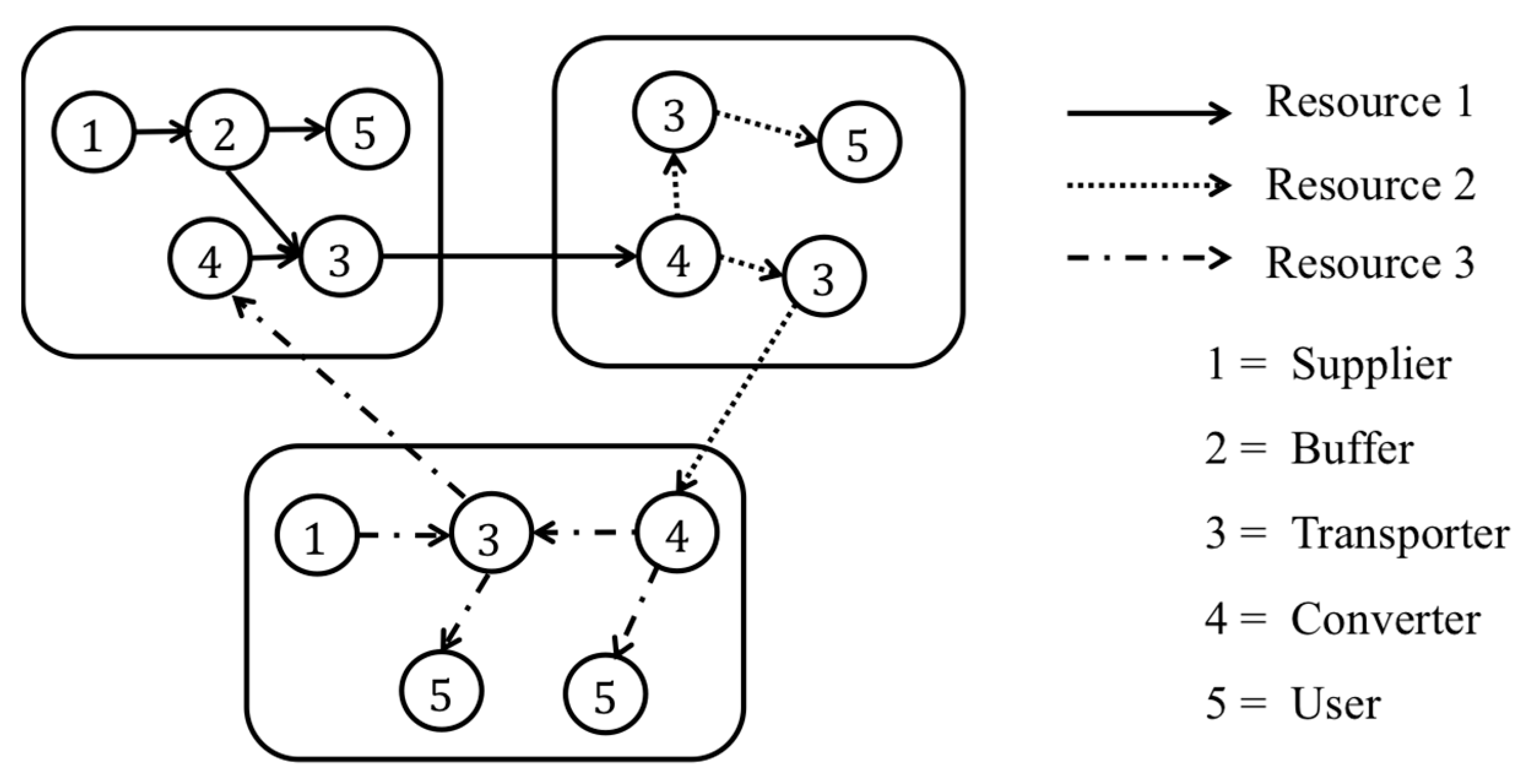
2.1. Modeling Approach
2.2. System Parameters
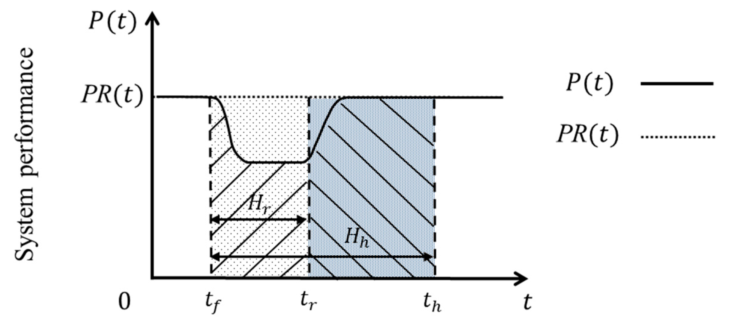
2.3. System Resilience Metric
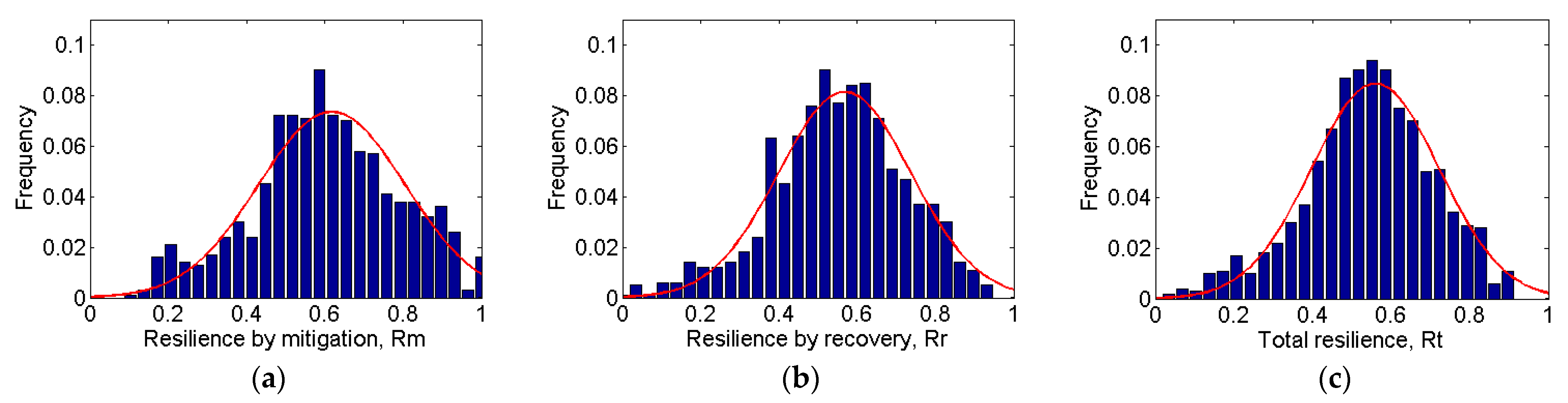
2.4. Resilience Indicators for ICIs
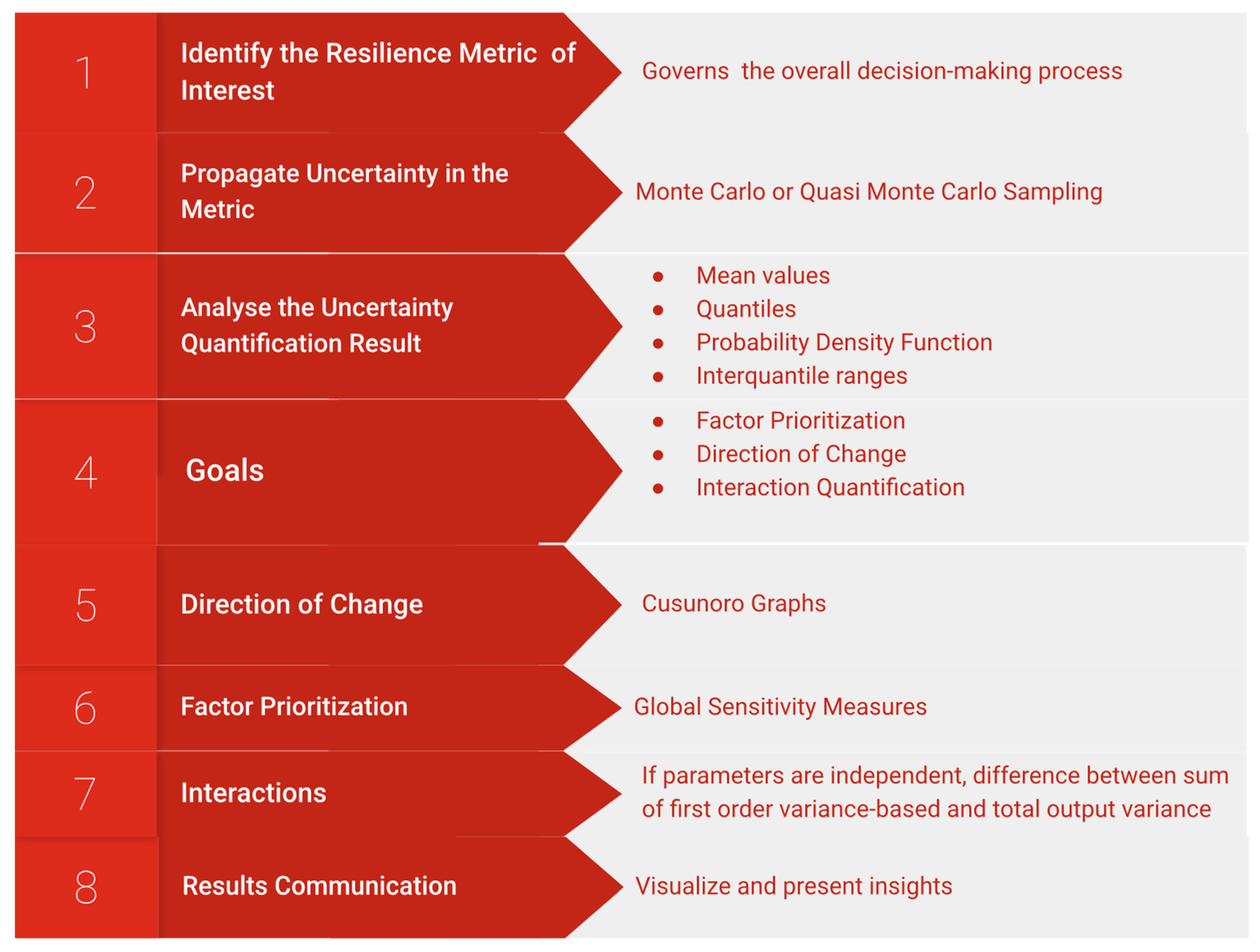
3. Global Sensitivity Approach
3.1. A General Framework for Global Sensitivity Methods
3.2. Computational Issues of Global Sensitivity Methods
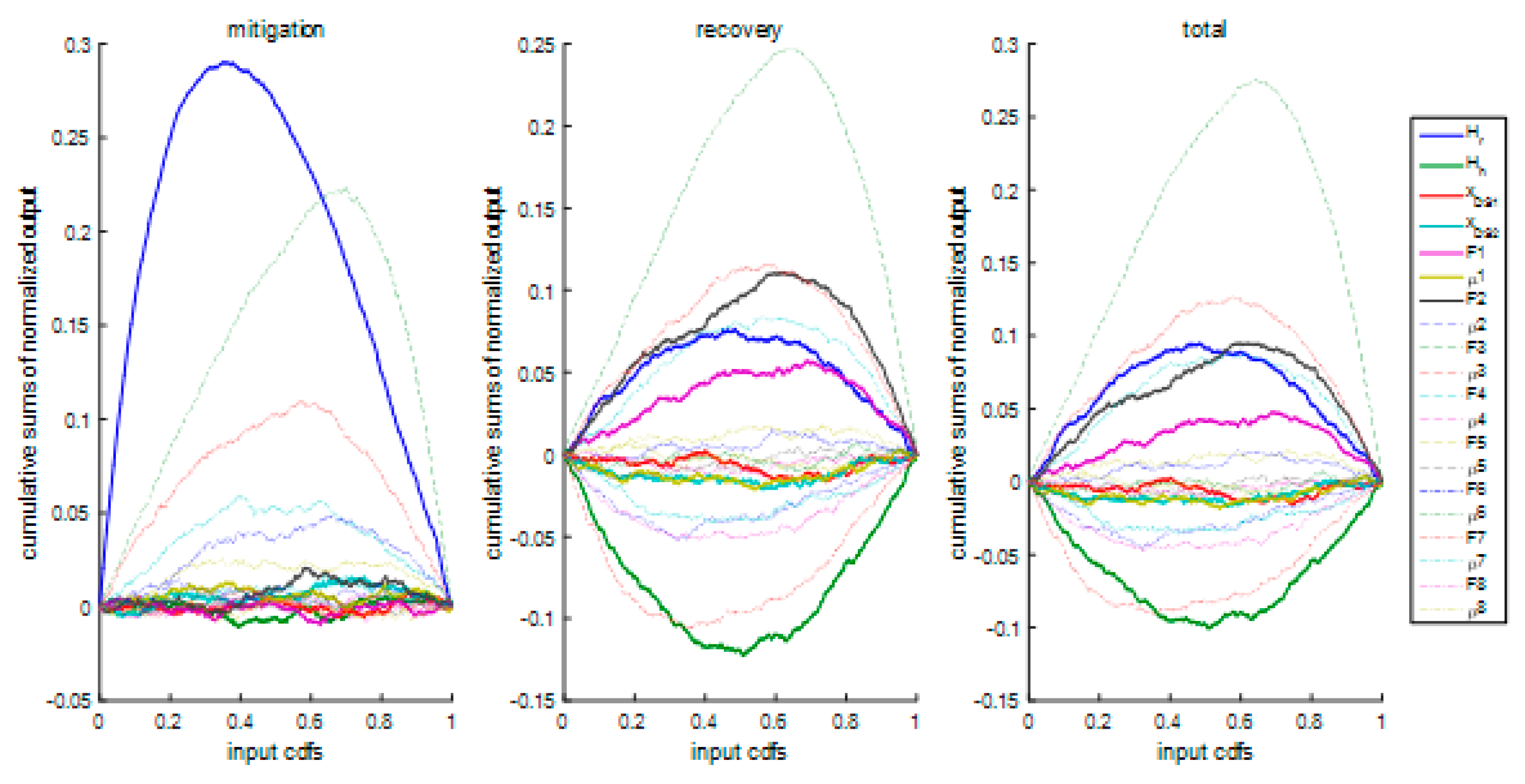
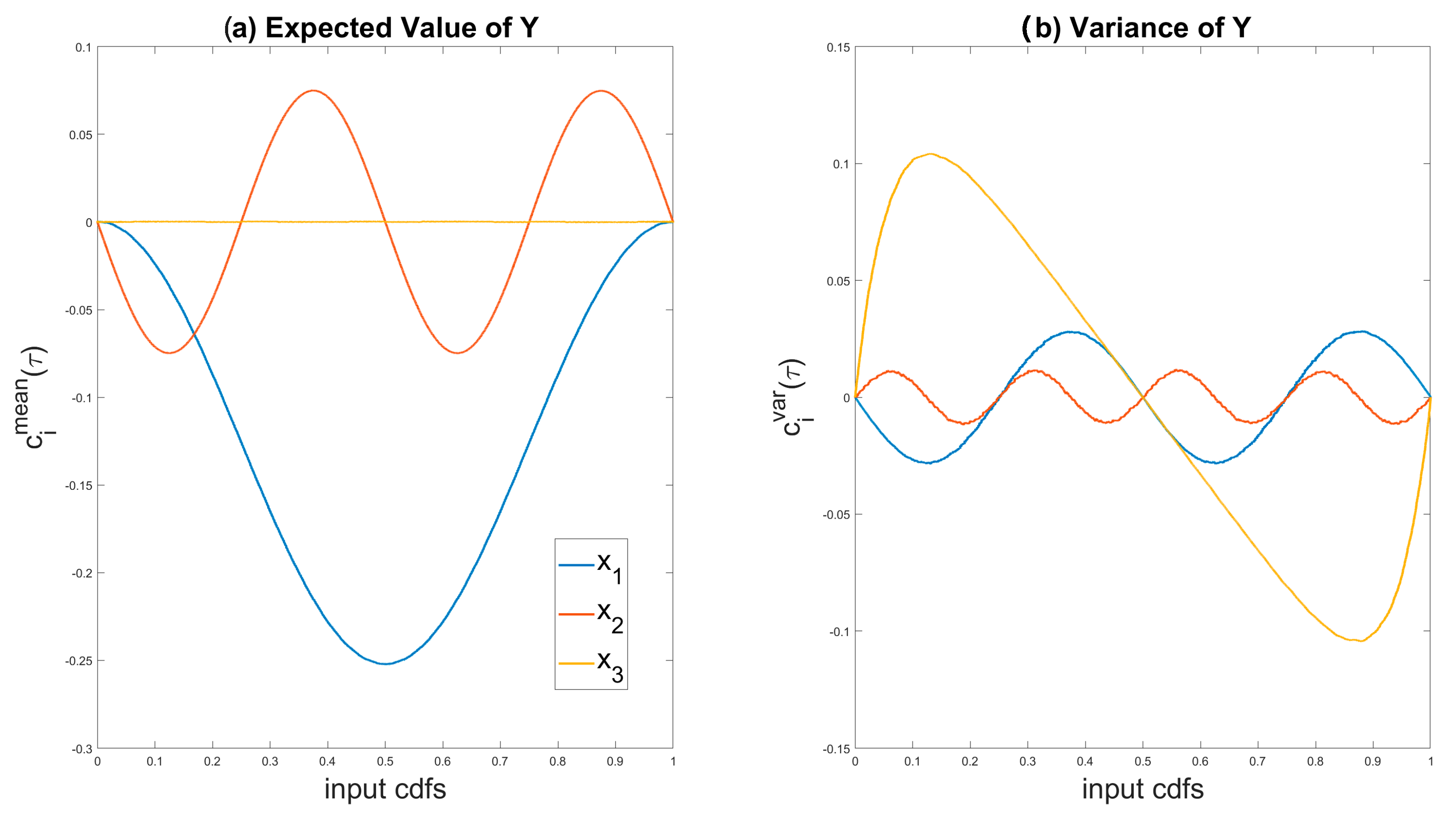
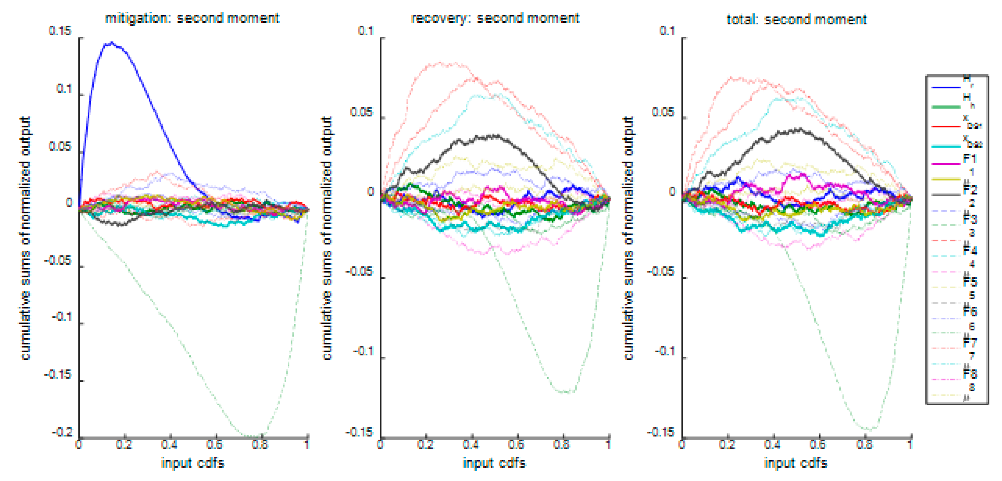
3.3. Visual Tools for Sensitivity Analysis
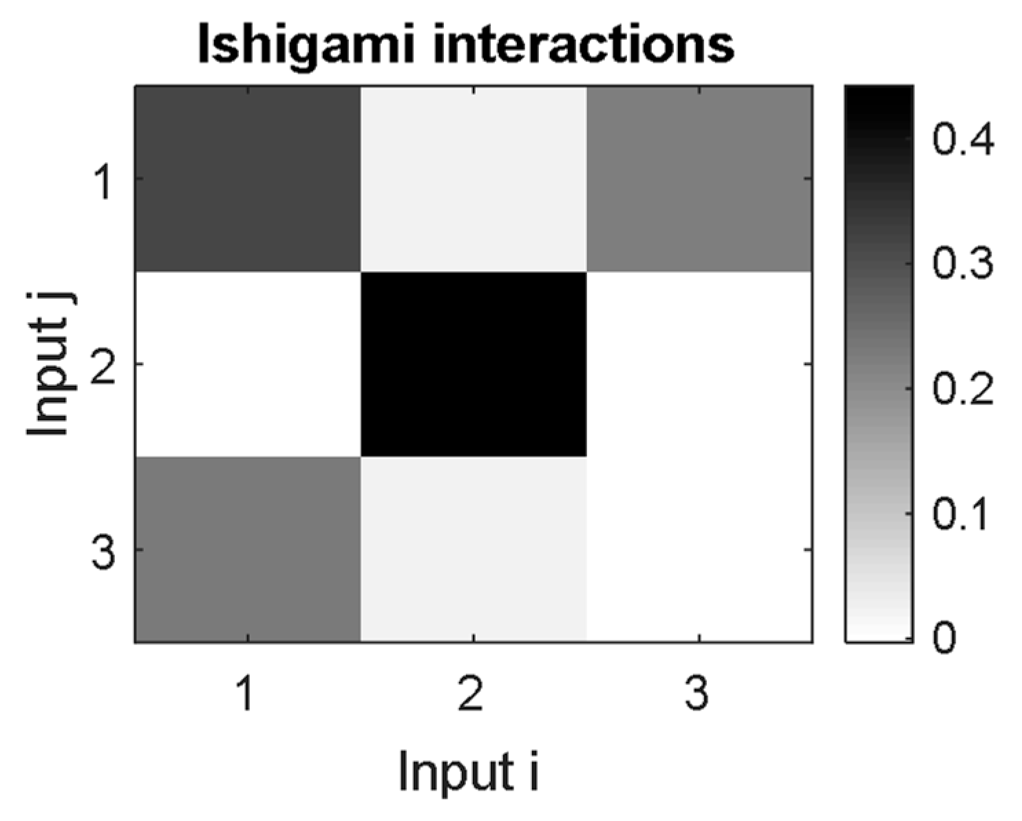
3.4. A Tool for Interaction Analysis
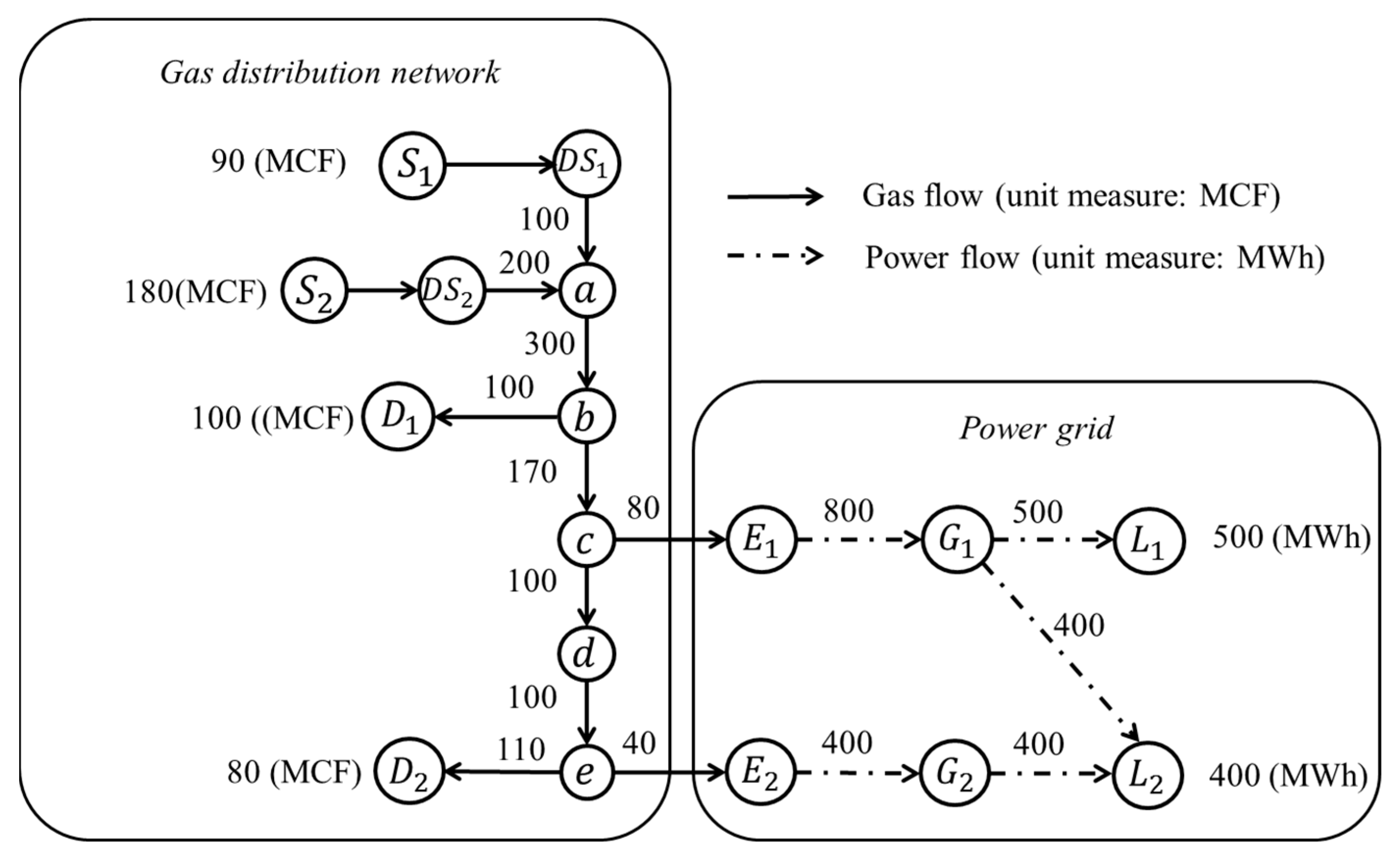
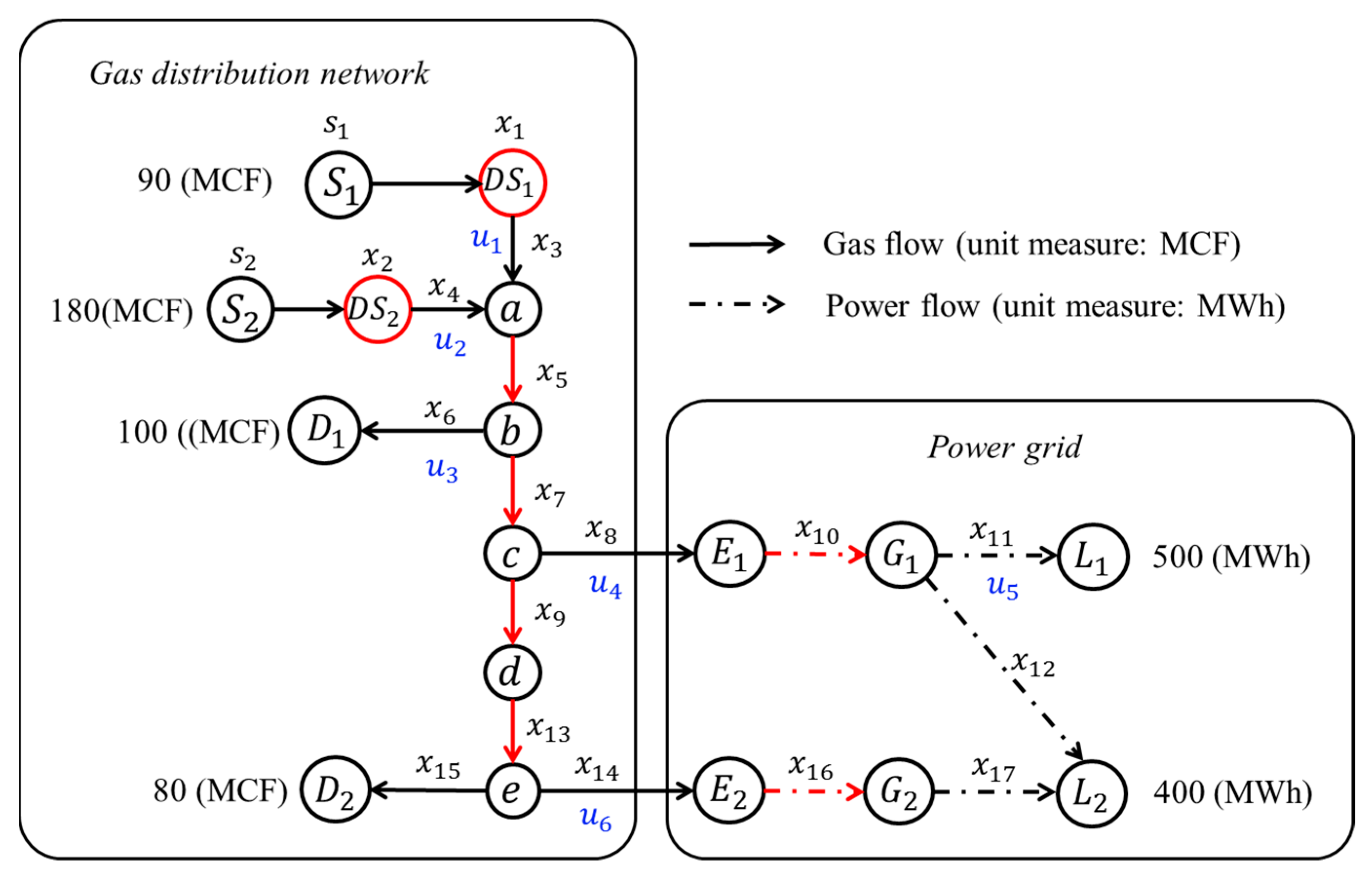
4. Case Study
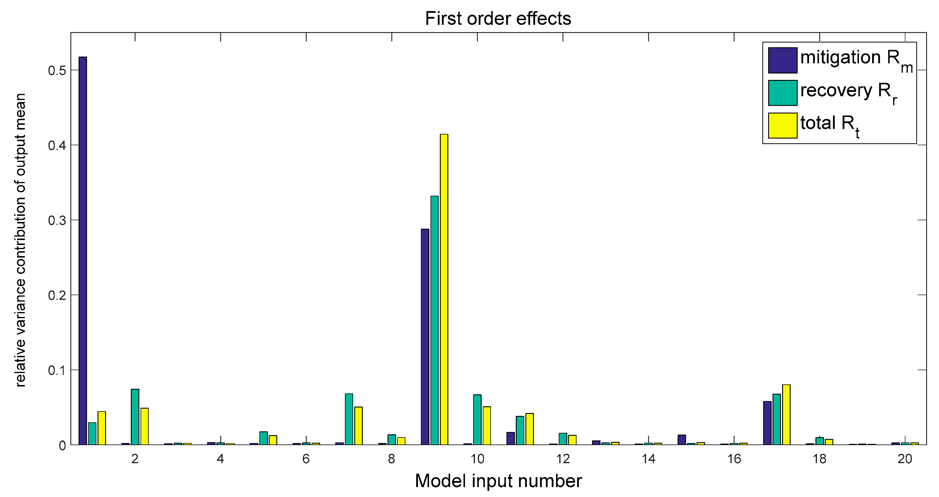
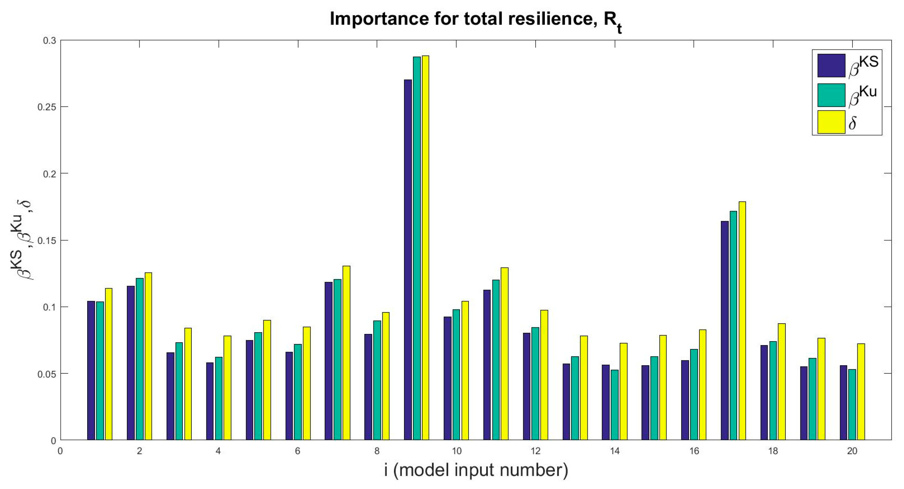
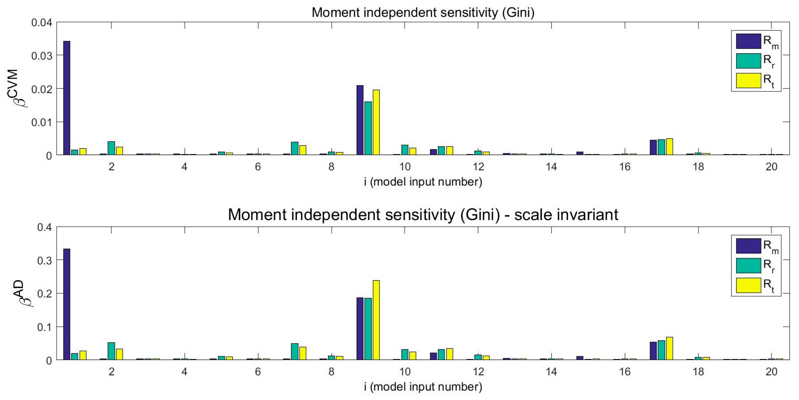
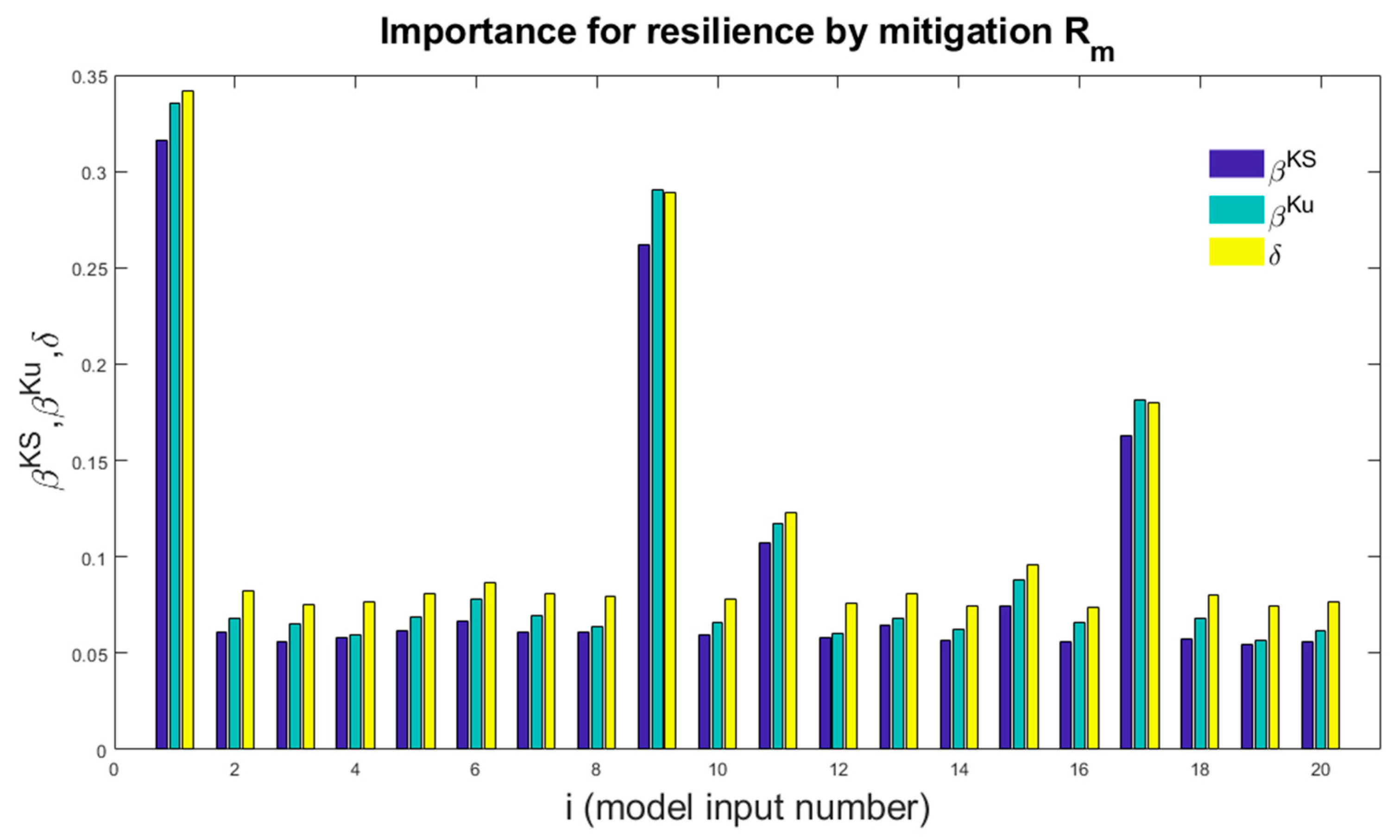
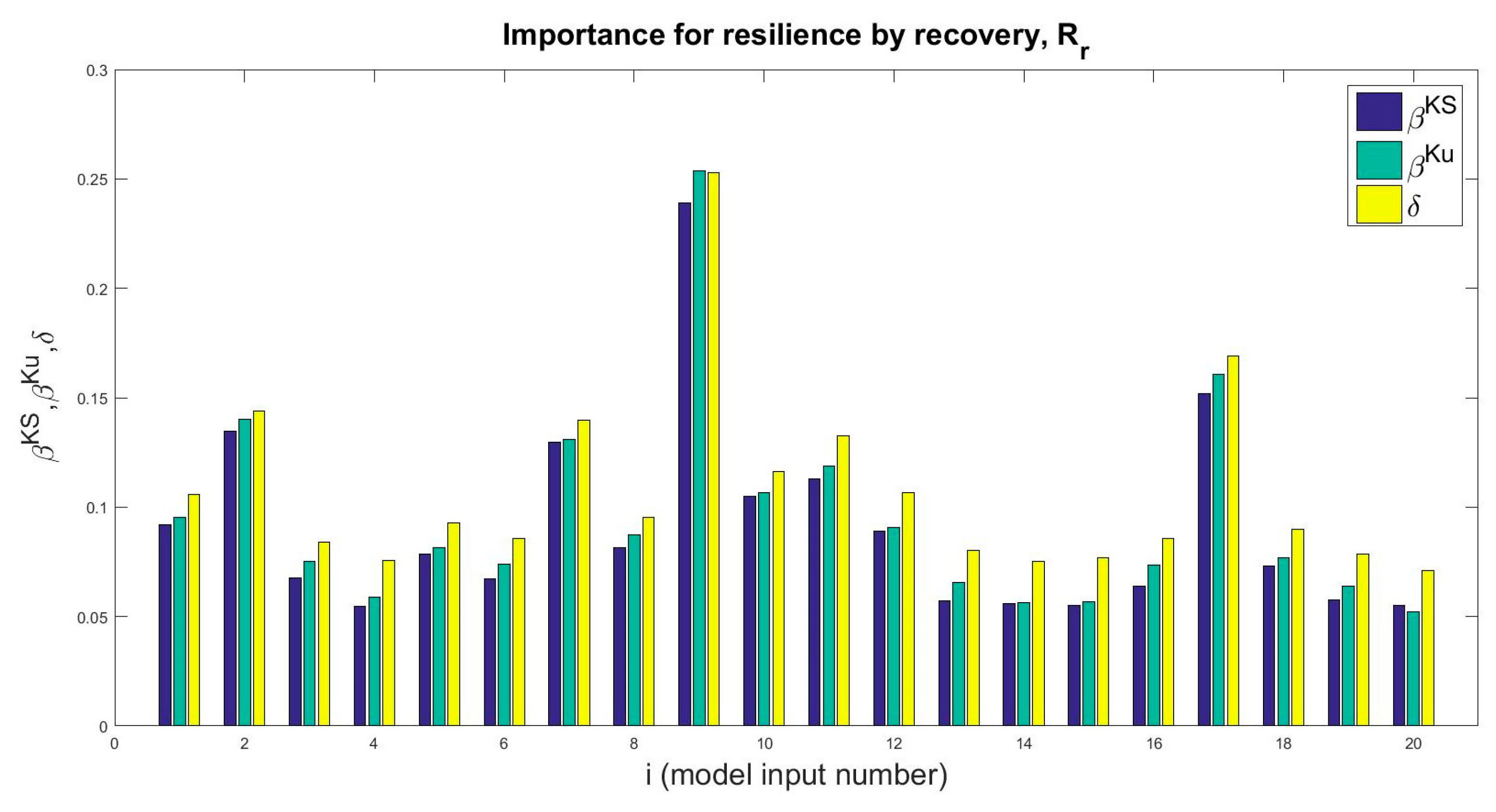
5. Sensitivity Analysis Results
6. Discussion and Interpretation
7. Conclusions
Supplementary Materials
Author Contributions
Funding
Data Availability Statement
Conflicts of Interest
References
- Protecting America’s Infrastructures: The Report of the President’s Commission on Critical Infrastructure Protection; The President’s Commission on Critical Infrastructure Protection: Washington, DC, USA, 1997.
- Mottahedi, A.; Sereshki, F.; Ataei, M.; Qarahasanlou, A.N.; Barabadi, A. The Resilience of Critical Infrastructure Systems: A Systematic Literature Review. Energies 2021, 14, 1571. [Google Scholar] [CrossRef]
- EU Commission. Communication from the Commission on a European Programme for Critical Infrastructure Protection; Commission of the European Communities: Brussels, Belgium, 2006. [Google Scholar]
- Lau, D.L.; Tang, A.; Pierre, J.-R. Performance of lifelines during the 1994 Northridge earthquake. Can. J. Civ. Eng. 1995, 22, 438–451. [Google Scholar] [CrossRef]
- Bao-Hua, Y.; Li-Li, X.; En-Jie, H. A comprehensive study method for lifeline system interaction under seismic conditions. Acta Seismol. Sin. 2004, 17, 211–221. [Google Scholar] [CrossRef]
- Kröger, W.; Zio, E. Vulnerable Systems; Springer: London, UK, 2011. [Google Scholar]
- Yates, A. A framework for studying mortality arising from critical infrastructure loss. Int. J. Crit. Infrastruct. Prot. 2014, 7, 100–111. [Google Scholar] [CrossRef]
- Zio, E. Challenges in the vulnerability and risk analysis of critical infrastructures. Reliab. Eng. Syst. Saf. 2016, 152, 137–150. [Google Scholar] [CrossRef]
- Reed, D.A.; Kapur, K.C.; Christie, R.D. Methodology for assessing the resilience of networked infrastructure. IEEE Syst. J. 2009, 3, 174–180. [Google Scholar] [CrossRef]
- Vugrin, E.D.; Camphouse, R.C. Infrastructure resilience assessment through control design. Int. J. Crit. Infrastruct. 2011, 7, 243. [Google Scholar] [CrossRef]
- Linkov, I.; Eisenberg, D.A.; Plourde, K.; Seager, T.P.; Allen, J.; Kott, A. Resilience metrics for cyber systems. Environ. Syst. Decis. 2013, 33, 471–476. [Google Scholar] [CrossRef]
- Cimellaro, G.P.; Reinhorn, A.M.; Bruneau, M. Framework for analytical quantification of disaster resilience. Eng. Struct. 2010, 32, 3639–3649. [Google Scholar] [CrossRef]
- Ouyang, M.; Dueñas-Osorio, L.; Min, X. A three-stage resilience analysis framework for urban infrastructure systems. Struct. Saf. 2012, 36–37, 23–31. [Google Scholar] [CrossRef]
- Pederson, P.; Dudenhoeffer, D.; Hartley, S.; Permann, M. Critical Infrastructure Interdependency Modeling: A Survey of U.S. and International Research. Ida. Natl. Lab. 2006, 25, 27. [Google Scholar] [CrossRef]
- Rinaldi, S.; Peerenboom, J.; Kelly, T. Identifying, understanding, and analyzing critical infrastructure interdependencies. IEEE Control Syst. Mag. 2001, 21, 11–25. [Google Scholar] [CrossRef]
- Rinaldi, S.M. Modeling and simulating critical infrastructures and their interdependencies. In Proceedings of the 37th Annual Hawaii International Conference on System Sciences, Big Island, HI, USA, 5–8 January 2004; pp. 1–8. [Google Scholar] [CrossRef]
- Liu, X.; Ferrario, E.; Zio, E. Resilience analysis framework for interconnected critical infrastructures. ASME J. Risk Uncertain. Eng. Syst. Part B Mech. Eng. 2017, 3, 021001. [Google Scholar] [CrossRef]
- Iman, R.L.; Helton, J.C.; Campbell, J.E. Risk Methodology for Geologic Disposal of Radioactive Waste: Sensitivity Analysis Techniques; Nuclear Regulatory Commission: Rockville, MD, USA, 1978. [Google Scholar]
- Iman, R.L.; Hora, S.C. A Robust Measure of Uncertainty Importance for Use in Fault Tree System Analysis. Risk Anal. 1990, 10, 401–406. [Google Scholar] [CrossRef]
- Helton, J.C.; Davis, F.J. Illustration of Sampling-Based Methods for Uncertainty and Sensitivity Analysis. Risk Anal. 2002, 22, 591–622. [Google Scholar] [CrossRef] [PubMed]
- Saltelli, A. Sensitivity Analysis for Importance Assessment. Risk Anal. 2002, 22, 579–590. [Google Scholar] [CrossRef] [PubMed]
- Patil, S.R.; Frey, H. Comparison of Sensitivity Analysis Methods Based on Applications to a Food Safety Risk Assessment Model. Risk Anal. 2004, 24, 573–585. [Google Scholar] [CrossRef]
- Lamboni, M.; Sanaa, M.; Tenenhaus-Aziza, F. Sensitivity analysis for critical control points determination and uncertainty analysis to link FSO and process criteria: Application to listeria monocytogenes in soft cheese made from pasteurized milk. Risk Anal. 2014, 34, 751–764. [Google Scholar] [CrossRef] [PubMed]
- Iman, R.L.; Johnson, M.E.; Watson, C.C.J. Sensitivity Analysis for Computer Model Projections of Hurricane Losses. Risk Anal. 2005, 25, 1277–1298. [Google Scholar] [CrossRef]
- Anderson, B.; Borgonovo, E.; Galeotti, M.; Roson, R. Uncertainty in Climate Change Modelling: Can Global Sensitivity Analysis be of Help? Risk Anal. 2014, 34, 271–293. [Google Scholar] [CrossRef]
- Koks, E.E.; Bockarjova, M.; de Moel, H.; Aerts, J.C.J.H. Integrated direct and indirect flood risk modeling: Development and sensitivity analysis. Risk Anal. 2015, 35, 882–900. [Google Scholar] [CrossRef] [PubMed]
- Cucurachi, S.; Borgonovo, E.; Heijungs, R. A Potocol for the Global Sensitivity Analysis of Impact Assessment Models in Life Cycle Assessment. Risk Anal. 2016, 36, 357–377. [Google Scholar] [CrossRef] [PubMed]
- Lee, E.E.; Mitchell, J.E.; Wallace, W.A. Restoration of services in interdependent infrastructure systems: A network flows approach. IEEE Trans. Syst. Man Cybern. Part C Appl. Rev. 2007, 37, 1303–1317. [Google Scholar] [CrossRef]
- Nozick, L.K.; Turnquist, M.A.; Jones, D.A.; Davis, R.D.; Lawton, C.R. Assessing the performance of interdependent infrastructures and optimising investments. Int. J. Crit. Infrastruct. 2005, 1, 144–154. [Google Scholar] [CrossRef]
- Svendsen, N.K.; Wolthusen, S.D. Connectivity models of interdependency in mixed-type critical infrastructure networks. Inf. Secur. Tech. Rep. 2007, 12, 44–55. [Google Scholar] [CrossRef]
- Prodan, I.; Zio, E. A model predictive control framework for reliable microgrid energy management. Int. J. Electr. Power Energy Syst. 2014, 61, 399–409. [Google Scholar] [CrossRef]
- Saltelli, A.; Ratto, M.; Andres, T.; Campolongo, F.; Cariboni, J.; Gatelli, D.; Saisana, M.; Tarantola, S. Global Sensitivity Analysis. The Primer; John Wiley & Sons, Ltd.: Chichester, UK, 2008. [Google Scholar]
- Saltelli, A.; Tarantola, S.; Campolongo, F. Sensitivity Analysis as an Ingredient of Modelling. Stat. Sci. 2000, 19, 377–395. [Google Scholar]
- Borgonovo, E.; Hazen, G.; Plischke, E. A Common Rationale for Global Sensitivity Measures and their Estimation. Risk Anal. 2016, 36, 1871–1895. [Google Scholar] [CrossRef] [PubMed]
- Borgonovo, E. A New Uncertainty Importance Measure. Reliab. Eng. Syst. Saf. 2007, 92, 771–784. [Google Scholar] [CrossRef]
- Baucells, M.; Borgonovo, E. Invariant Probabilistic Sensitivity Analysis. Manag. Sci. 2013, 59, 2536–2549. [Google Scholar] [CrossRef]
- Borgonovo, E.; Tarantola, S.; Plischke, E.; Morris, M.D. Transformation and Invariance in the Sensitivity Analysis of Computer Experiments. J. R. Stat. Soc. Ser. B 2014, 76, 925–947. [Google Scholar] [CrossRef]
- Gamboa, F.; Klein, T.; Lagnoux, A. Sensitivity Analysis Based on Cramer von Mises Distance. SIAM/ASA J. Uncertain. Quantif. 2018, 6, 522–548. [Google Scholar] [CrossRef]
- Da Veiga, S. Global Sensitivity Analysis with Dependence Measures. J. Stat. Comput. Simul. 2015, 85, 1283–1305. [Google Scholar] [CrossRef]
- De Lozzo, M.; Marrel, A. New improvements in the use of dependence measures for sensitivity analysis and screening. J. Stat. Comput. Simul. 2016, 86, 3038–3058. [Google Scholar] [CrossRef]
- De Lozzo, M.; Marrel, A. Sensitivity analysis with dependence and variance-based measures for spatio-temporal numerical simulators. Stoch. Environ. Res. Risk Assess. 2017, 31, 1437–1453. [Google Scholar] [CrossRef]
- Plischke, E.; Borgonovo, E. Fighting the Curse of Sparsity: Probabilistic Sensitivity Measures from Cumulative Distribution Functions. Risk Anal. 2020, 40, 2639–2660. [Google Scholar] [CrossRef] [PubMed]
- Soboĺ, I.M. Sensitivity Estimates for Nonlinear Mathematical Models. Math. Model. Comput. Exp. 1993, 1, 407–414. [Google Scholar]
- Gamboa, F.; Janon, A.; Klein, T.; Lagnoux, A.; Prieur, C. Statistical inference for Sobol pick-freeze Monte Carlo method. Statistics 2016, 50, 881–902. [Google Scholar] [CrossRef]
- Pearson, K. On the General Theory of Skew Correlation and Non-linear Regression; Dulau and Company: London, UK, 1905; Volume XIV. [Google Scholar]
- Kleijnen, J.P.C.; Helton, J.C. Statistical analyses of scatterplots to identify important factors in large-scale simulations, 1: Review and comparison of techniques. Reliab. Eng. Saf. 1999, 65, 147–185. [Google Scholar] [CrossRef]
- Strong, M.; Oakley, J.E.; Chilcott, J. Managing Structural Uncertainty in Health Economic Decision Models: A Discrepancy Approach. J. R. Stat. Soc. Ser. C 2012, 61, 25–45. [Google Scholar] [CrossRef]
- Strong, M.; Oakley, J.E. An Efficient Method for Computing Partial Expected Value of Perfect Information for Correlated Inputs. Med. Decis. 2013, 33, 755–766. [Google Scholar] [CrossRef] [PubMed]
- Strong, M.; Oakley, J.E.; Brennan, A.; Breeze, P. Estimating the Expected Value of Sample Information Using the Probabilistic Sensitivity Analysis Sample. Med. Decis. Mak. 2015, 35, 570–583. [Google Scholar] [CrossRef] [PubMed]
- Soboĺ, I.M. On the distribution of points in a cube and the approximate evaluation of integrals. USSR Comput. Math. Math. Phys. 1969, 7, 86–112. [Google Scholar] [CrossRef]
- Ökten, G.; Liu, Y. Randomized quasi-Monte Carlo methods in global sensitivity analysis. Reliab. Eng. Syst. Saf. 2021, 210, 107520. [Google Scholar] [CrossRef]
- Owen, A.B. Halton sequences avoid the origin. SIAM Rev. 2006, 48, 487–503. [Google Scholar] [CrossRef]
- Owen, A.B. Latin supercube sampling for very high-dimensional simulations. ACM Trans. Model. Comput. Simul. 1998, 8, 71–102. [Google Scholar] [CrossRef]
- Damblin, G.; Ghione, A. Adaptive use of replicated Latin Hypercube Designs for computing Soboĺ sensitivity indices. Reliab. Eng. Syst. Saf. 2021, 212, 107507. [Google Scholar] [CrossRef]
- Plischke, E. An Adaptive Correlation Ratio Method Using the Cumulative Sum of the Reordered Output. Reliab. Eng. Syst. Saf. 2012, 107, 149–156. [Google Scholar] [CrossRef]
- Ishigami, T.; Homma, T. An Importance Quantification Technique in Uncertainty Analysis for Computer Models. In Proceedings of the First International Symposium on Uncertainty Modeling and Analysis, College Park, MD, USA, 3–5 December 1990; pp. 398–403. [Google Scholar] [CrossRef]
- Tarantola, S.; Kopustinskas, V.; Bolado-Lavin, R.; Kaliatka, A.; Ušpuras, E.; Vaišnoras, M. Sensitivity analysis using contribution to sample variance plot: Application to a water hammer model. Reliab. Eng. Syst. Saf. 2012, 99, 62–73. [Google Scholar] [CrossRef]
- Fort, J.-C.; Klein, T.; Rachdi, N. New Sensitivity Analysis Subordinated to a Contrast. Commun. Stat.-Theory Methods 2016, 45, 4349–4364. [Google Scholar] [CrossRef]
- Sudret, B. Global sensitivity analysis using polynomial chaos expansion. Reliab. Eng. Syst. Saf. 2008, 93, 964–979. [Google Scholar] [CrossRef]
- Plischke, E. An effective algorithm for computing global sensitivity indices (EASI). Reliab. Eng. Syst. Saf. 2010, 95, 354–360. [Google Scholar] [CrossRef]
- Lu, X.; Rudi, A.; Borgonovo, E.; Rosasco, L. Faster kriging: Facing high-dimensional simulators. Oper. Res. 2020, 68, 233–249. [Google Scholar] [CrossRef]


| Description | Symbol | Bounds | Unit Measure |
|---|---|---|---|
| Response time | Hr | [0, 30] | hours |
| Time horizon | Hh | [50, 100] | hours |
| The initial storage of the buffer DS1 | [1000, 4000] | MCF | |
| The initial storage of the buffer DS2 | [2000, 8000] | MCF |
| Vulnerable Element | Failure Magnitude Fi | Units of Fi | Recovery Rate μi | Units of μi | |
|---|---|---|---|---|---|
| 1 | Supplier | [0, 90] | MCF | [0, 1.8] | MCF/h |
| 2 | Supplier | [0, 180] | MCF | [0, 3.6] | MCF/h |
| 3 | Link | [0, 300] | MCF | [0, 6] | MCF/h |
| 4 | Link | [0, 170] | MCF | [0, 3.4] | MCF/h |
| 5 | Link | [0, 100] | MCF | [0, 2] | MCF/h |
| 6 | Link | [0, 100] | MCF | [0, 2] | MCF/h |
| 7 | Link | [0, 800] | MWh | [0, 16] | MWh/h |
| 8 | Link | [0, 400] | MWh | [0, 8] | MWh/h |
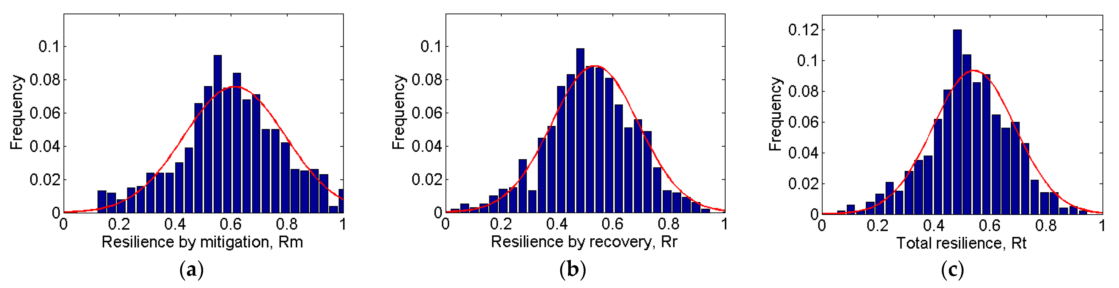
| Distribution of Resilience Indicators | Mean | Standard Deviation |
|---|---|---|
| Resilience by mitigation | 0.6121 | 0.1815 |
| Resilience by recovery | 0.5356 | 0.1557 |
| Total resilience | 0.5425 | 0.1471 |
| Distribution of Resilience Metrics | Mean | Standard Deviation |
|---|---|---|
| Resilience by mitigation | 0.6177 | 0.1874 |
| Resilience by recovery | 0.5678 | 0.1692 |
| Total resilience | 0.5597 | 0.1625 |
Disclaimer/Publisher’s Note: The statements, opinions and data contained in all publications are solely those of the individual author(s) and contributor(s) and not of MDPI and/or the editor(s). MDPI and/or the editor(s) disclaim responsibility for any injury to people or property resulting from any ideas, methods, instructions or products referred to in the content. |
© 2024 by the authors. Licensee MDPI, Basel, Switzerland. This article is an open access article distributed under the terms and conditions of the Creative Commons Attribution (CC BY) license (https://creativecommons.org/licenses/by/4.0/).
Share and Cite
Liu, X.; Zio, E.; Borgonovo, E.; Plischke, E. A Systematic Approach of Global Sensitivity Analysis and Its Application to a Model for the Quantification of Resilience of Interconnected Critical Infrastructures. Energies 2024, 17, 1823. https://doi.org/10.3390/en17081823
Liu X, Zio E, Borgonovo E, Plischke E. A Systematic Approach of Global Sensitivity Analysis and Its Application to a Model for the Quantification of Resilience of Interconnected Critical Infrastructures. Energies. 2024; 17(8):1823. https://doi.org/10.3390/en17081823
Chicago/Turabian StyleLiu, Xing, Enrico Zio, Emanuele Borgonovo, and Elmar Plischke. 2024. "A Systematic Approach of Global Sensitivity Analysis and Its Application to a Model for the Quantification of Resilience of Interconnected Critical Infrastructures" Energies 17, no. 8: 1823. https://doi.org/10.3390/en17081823
APA StyleLiu, X., Zio, E., Borgonovo, E., & Plischke, E. (2024). A Systematic Approach of Global Sensitivity Analysis and Its Application to a Model for the Quantification of Resilience of Interconnected Critical Infrastructures. Energies, 17(8), 1823. https://doi.org/10.3390/en17081823