

Investigation of Load, Solar and Wind Generation as Target Variables in LSTM Time Series Forecasting, Using Exogenous Weather Variables


Abstract
1. Introduction
- Our results have shown that weather data, used as exogenous variables within an LSTM framework, can have a significant positive impact on forecast accuracy for electricity load, solar and wind generation. It has been shown that careful consideration of a range of such variables is crucial for successful energy-related forecasting operations.
- Development of a framework for LSTM hyperparameter tuning for energy-related forecasting.
- Novel use of the seasonal component of a time series as a separate exogenous variable has been demonstrated to have potential utility as a possible LSTM training aid, as this improved accuracy metrics by a substantial margin.
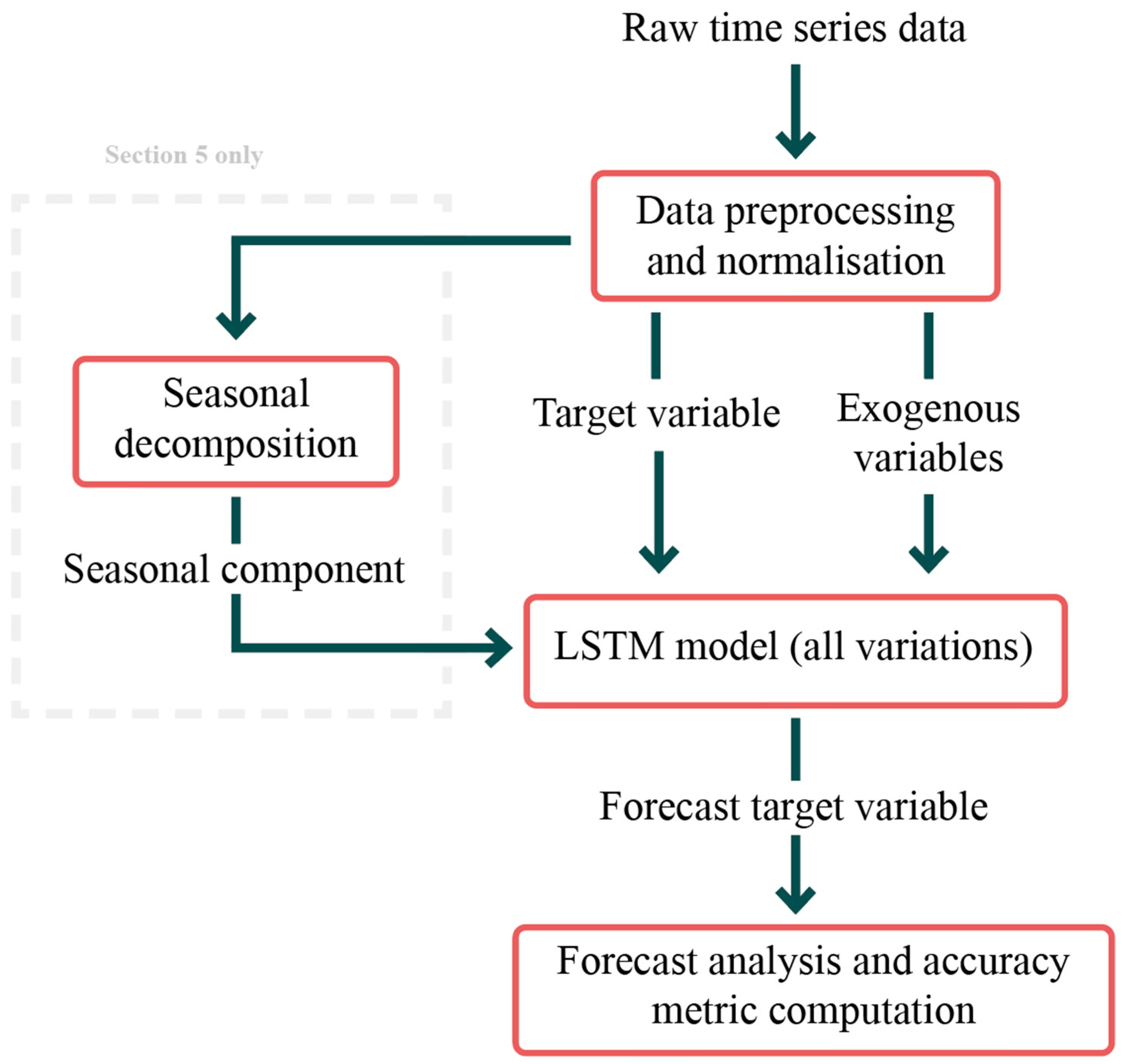
2. Proposed Methodology
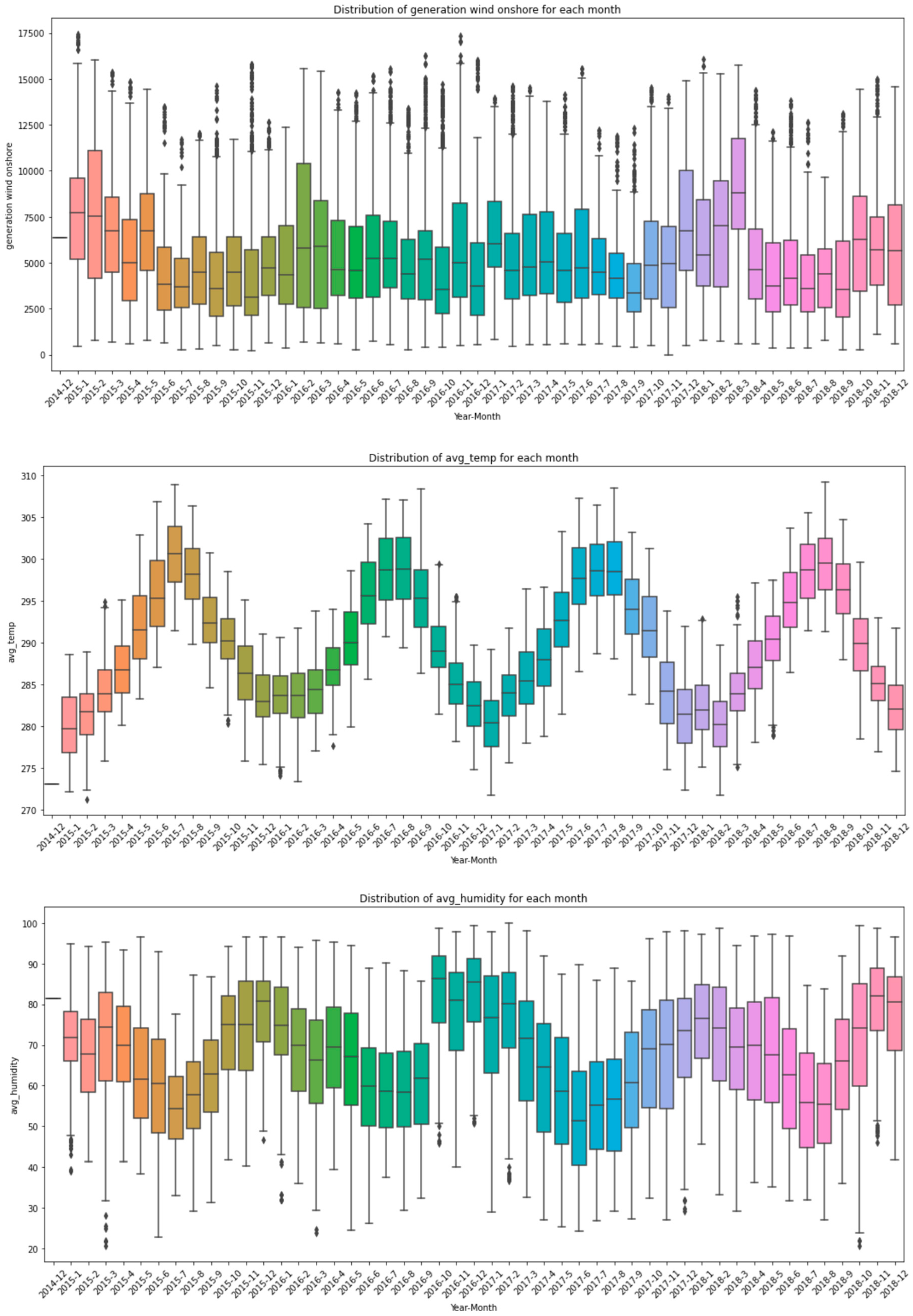
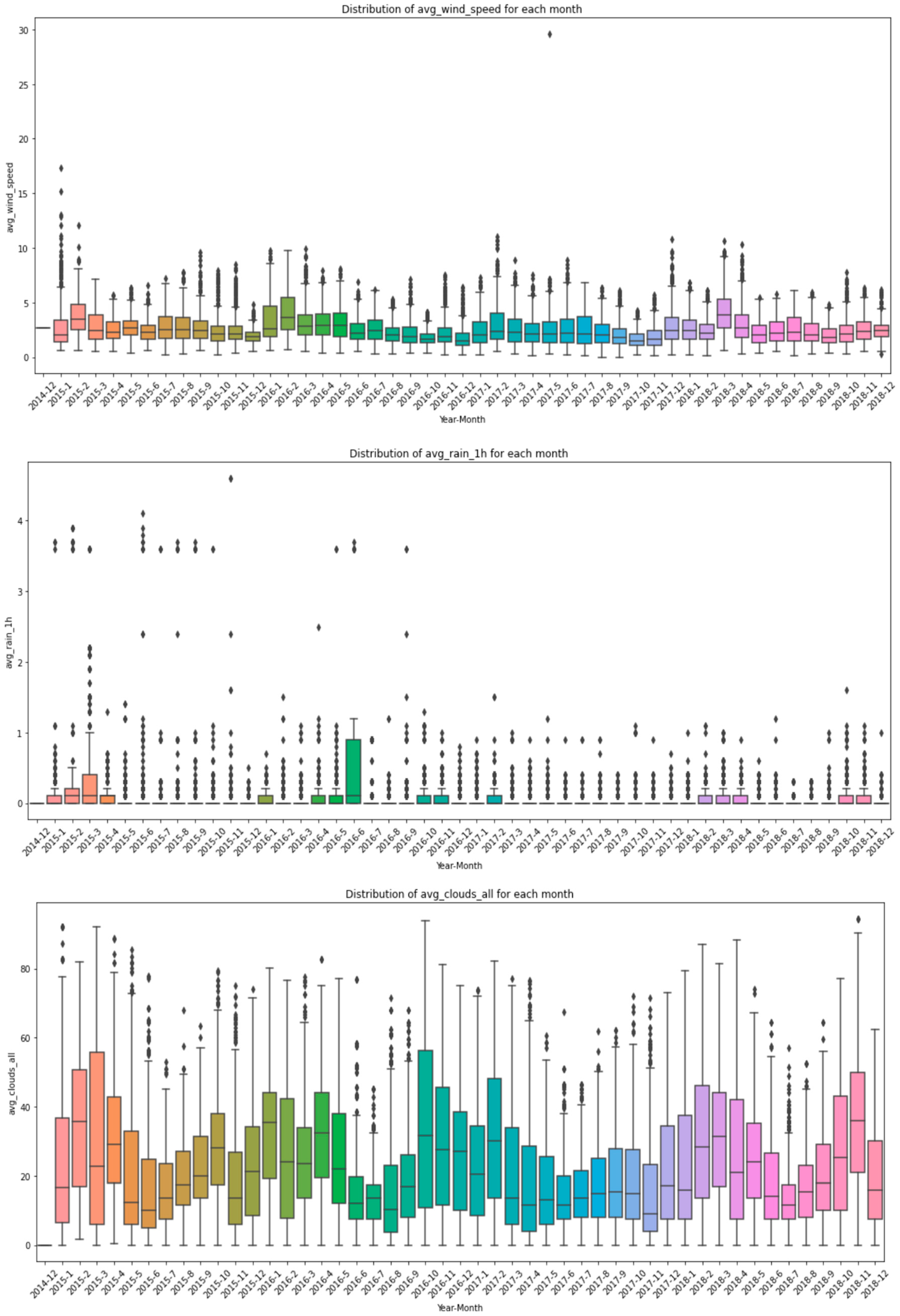
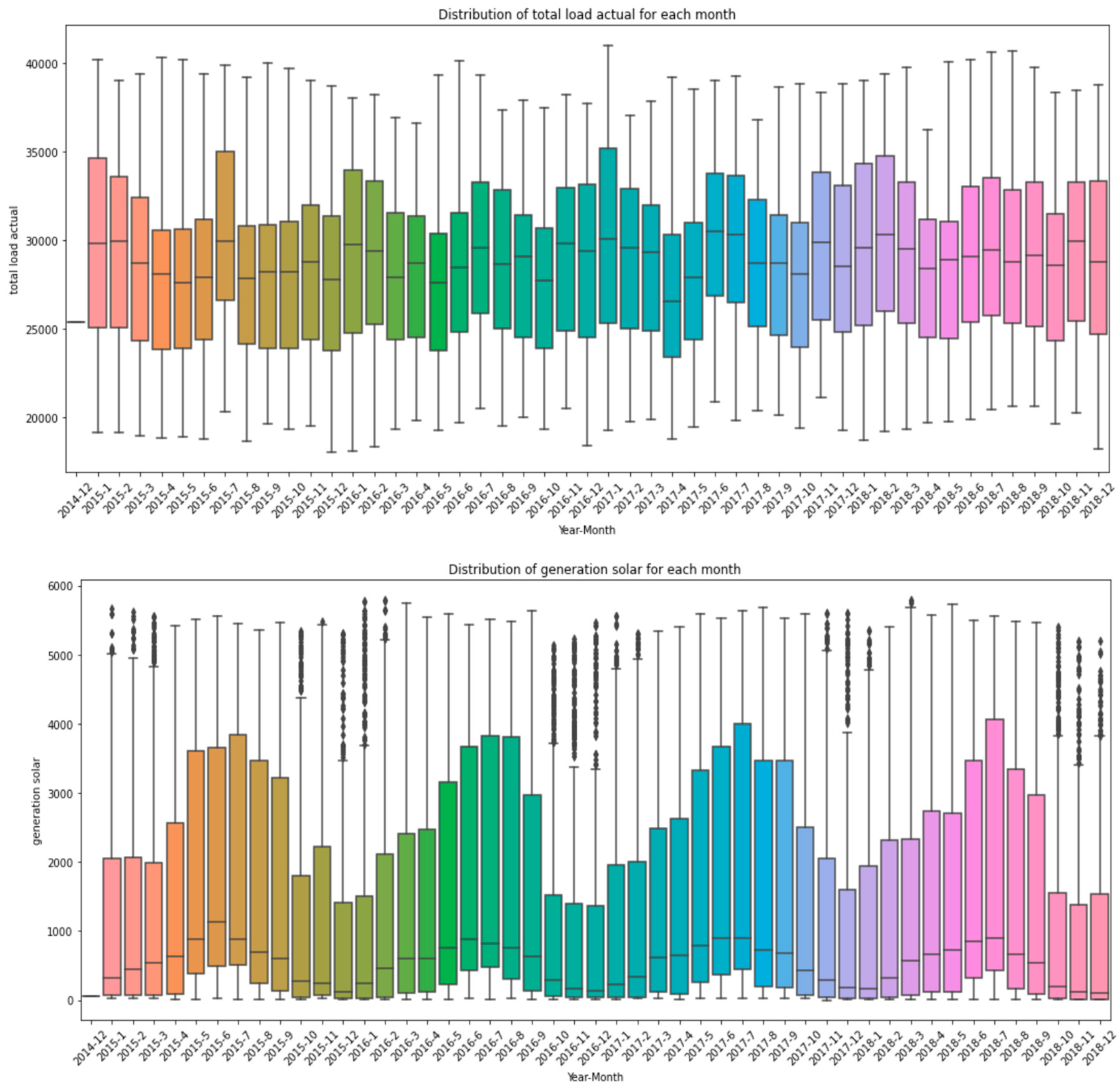
2.1. Input Data
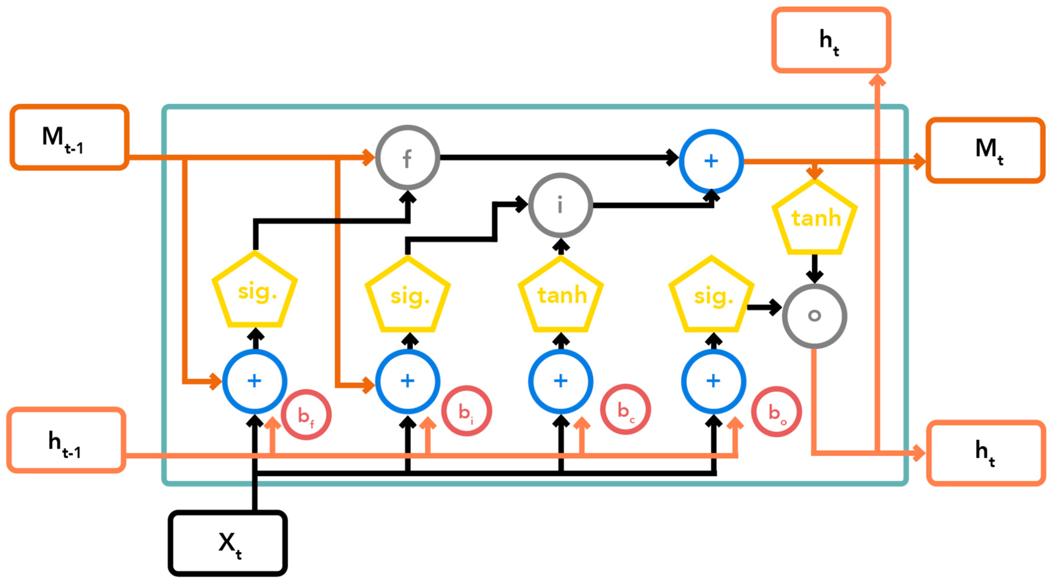
2.2. LSTM Basics
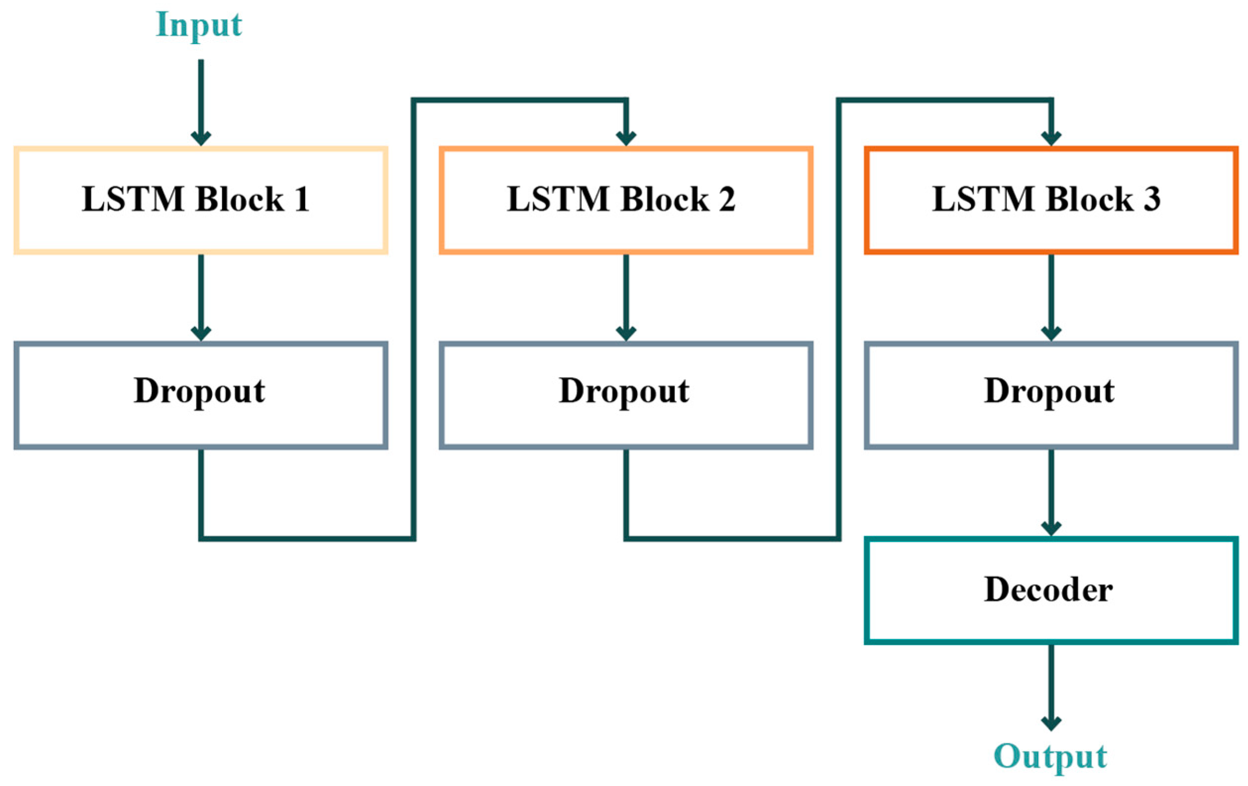
2.3. Proposed LSTM Architectures and Initialisation
2.4. Seasonal Decomposition
2.5. Evaluation Metrics
2.6. Initial Hyperparameter Optimisation
- −
- Optimiser weight decay = 1 × 10⁻⁶. This penalises large weights (the strength of the signal that a neuron will pass on to the next neuron in the network) in the neural network to avoid overfitting (when a model is unable to generalise to unseen data because it has fitted too closely the training data).
- −
- Batch size = 48. The number of data values in the time series processed before the model updates neuron weights in training. A lower value could potentially give more accurate predictions but the computational demand would increase. Furthermore, a lower value can make the model more ‘short-sighted’ to daily fluctuations, hence why a two-day period (48 h) was chosen.
- −
- The number of layers within an LSTM block = 2. Two layers within the LSTM block allow the block to capture more dependencies between data points compared to one layer. More layers led to a decrease in accuracy as the model likely overfitted.
- −
- A total of 200 epochs, the number of complete passes through all training data, during the training process, were used as this comfortably allowed convergence for training and validation loss. Therefore, discrepancies between training forecasts and the true values did not decrease further in a significant way after 200 passes.
3. Hyperparameter Cross-Validation and Model Evaluation
- −
- Hidden dimension size refers to the number of neuron units inside the hidden layer of an LSTM unit. Hidden dimension size adjustment was important to test because it helps to strike a balance between capturing enough information and not overfitting.
- −
- Learning rate, which affects how quickly neuron weights are updated during training, was selected as a key hyperparameter since the step size with which weights are updated is fundamental to convergence speed and accuracy, giving it a significant impact on performance. An optimal learning rate will provide a smooth progression towards the minimum test loss.
- −
- Dropout, the probability of a neuron in the dropout layer being deactivated temporarily during model training, is an easily implementable regularisation technique. It allows the model to better generalise by not relying heavily on any individual neuron and its associated connections. A dropout probability of 0.5, for example, would mean that 50% of neurons would be likely to be temporarily deactivated, forcing the model to function with the remaining 50%.
- −
- We experimented with three different optimisers: Adam, Root Mean Square Propagation (RMSProp) and Stochastic Gradient Descent (SGD), which are all commonly used algorithms that determine exactly how weights are updated during training. Optimiser functions can have a significant impact on model performance and convergence and depend greatly on other variables. As an example, the learning rate is a pivotal determinant of success for models using an SGD optimiser. Therefore, we thought it important to trial all possible hyperparameter combinations for each experiment.
- −
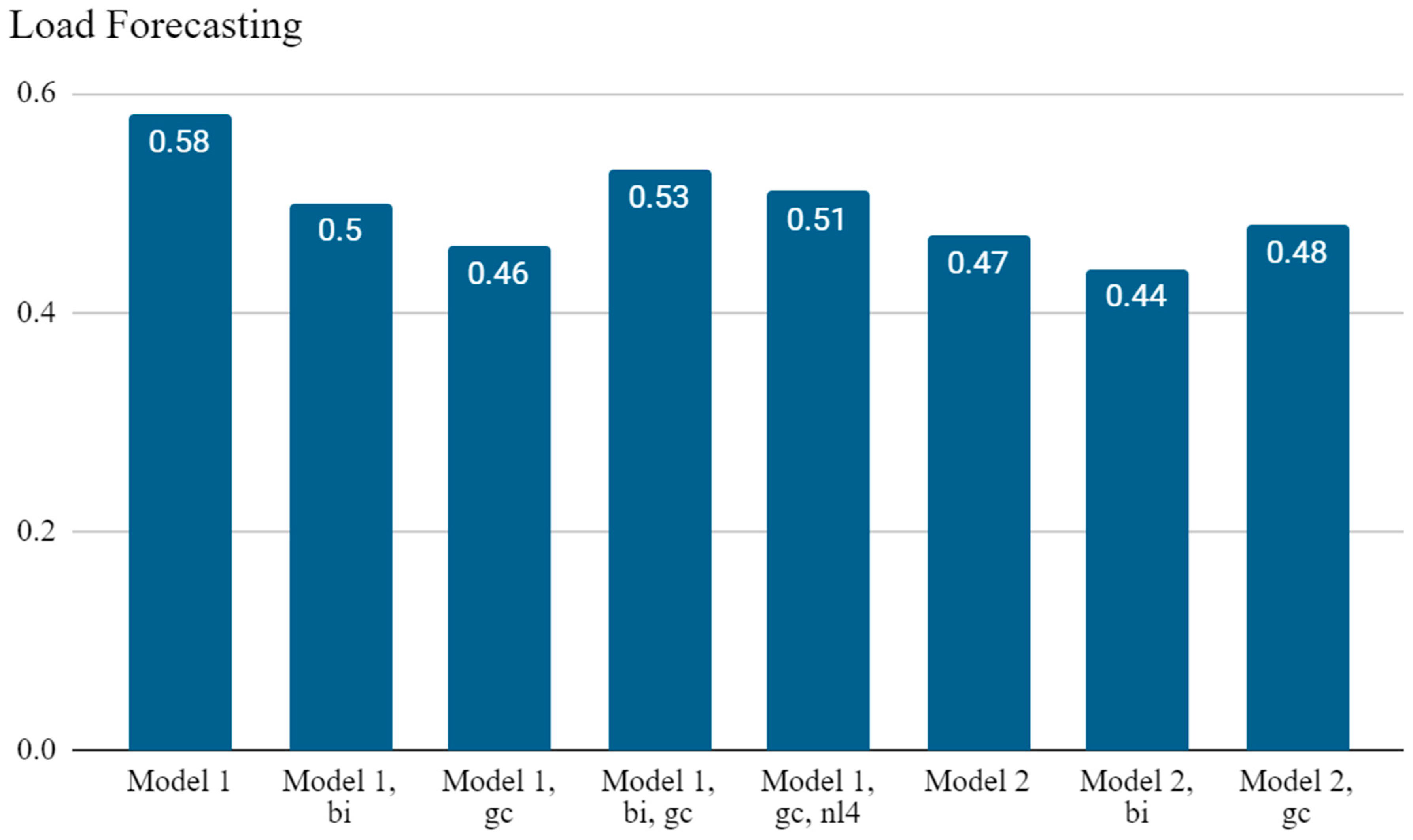
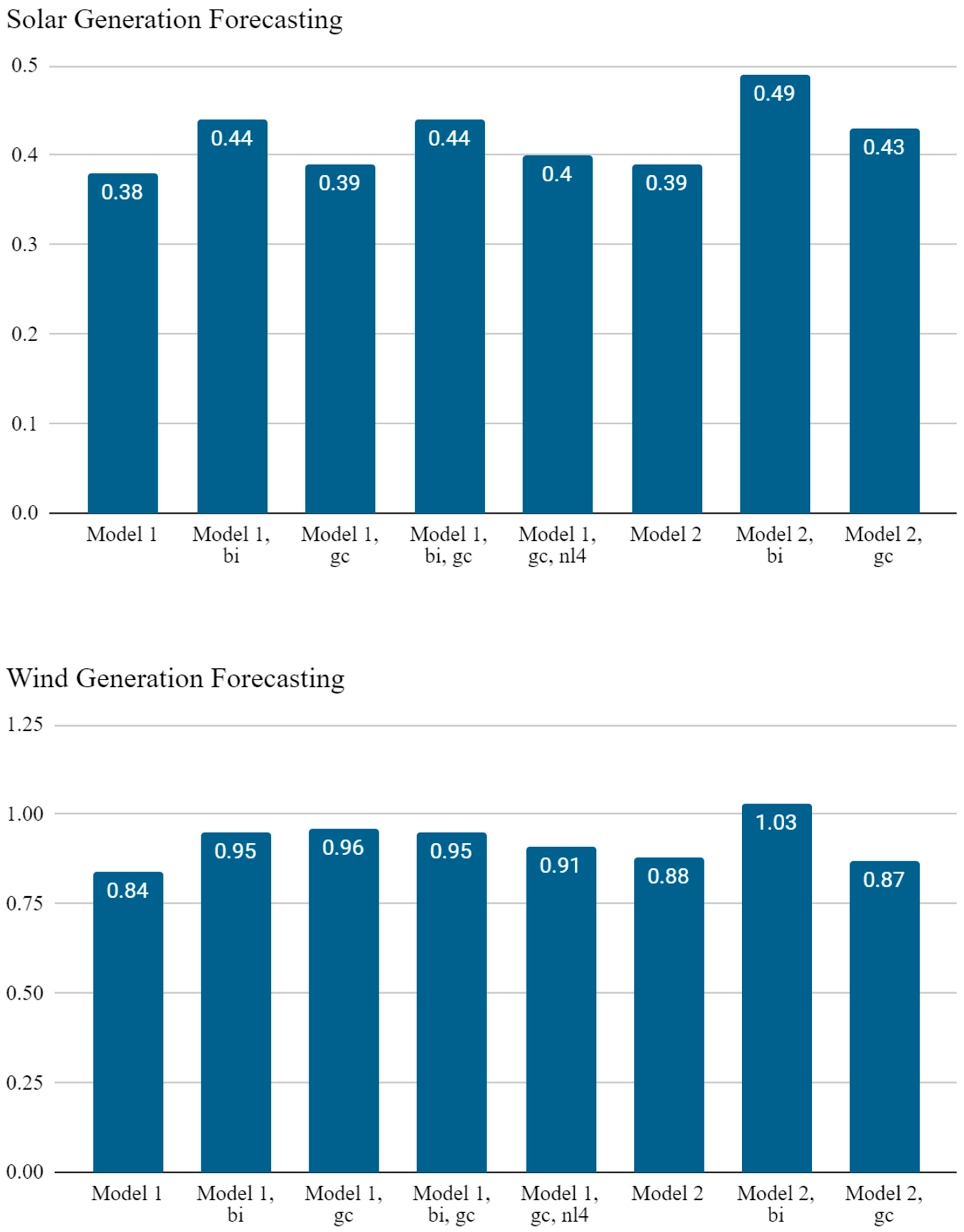
- Model 1 (Model 1);
- −
- Model 1 + bidirectional LSTM (Model 1, bi);
- −
- Model 1 + gradient clipping (Model 1, gc);
- −
- Model 1 + bidirectional LSTM + gradient clipping (Model 1, bi, gc);
- −
- Model 1 + gradient clipping + 4 LSTM block layers (Model 1, gc, nl4);
- −
- Model 2 (Model 2);
- −
- Model 2 + bidirectional LSTM (Model 2, bi);
- −
- Model 2 + gradient clipping (Model 2, gc);
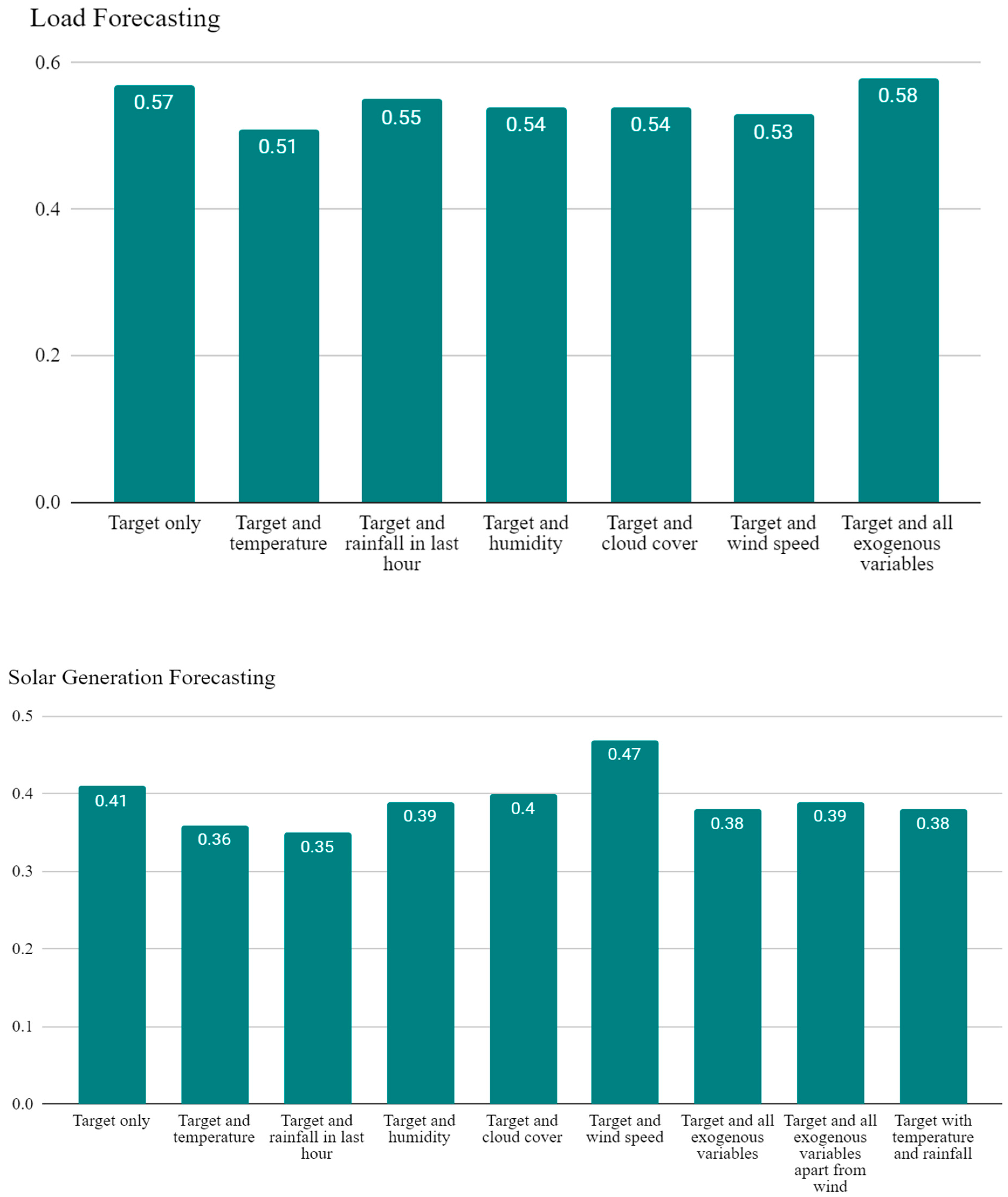
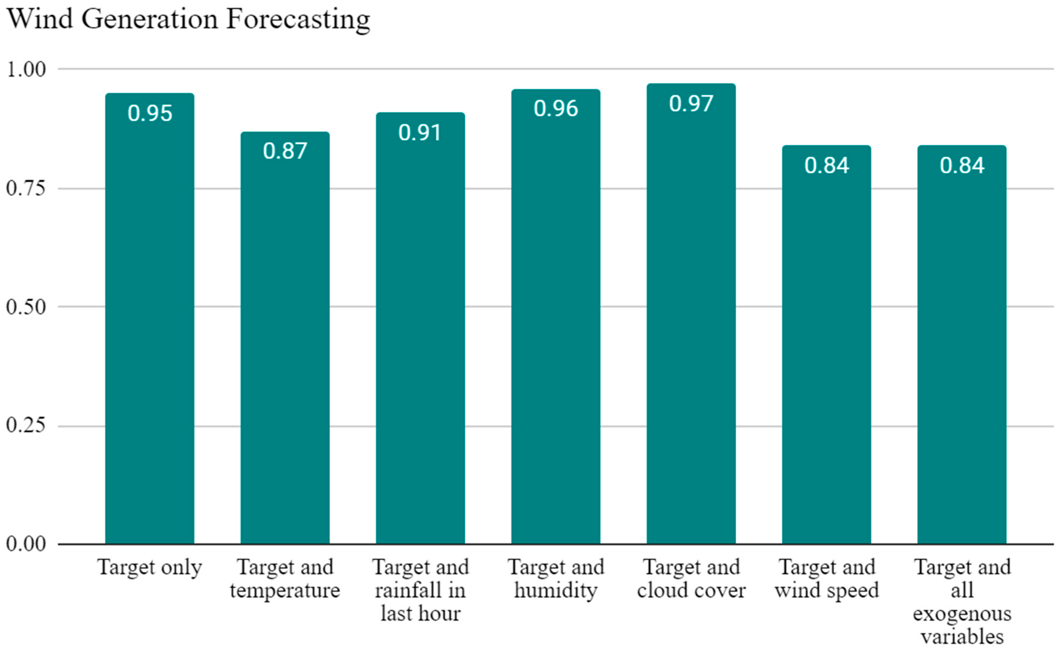
4. Exogenous Variable Analysis
- ~10% reduction in MASE and a ~14% decrease in test loss when load was forecast with an exogenous temperature variable (Appendix A Table A2).
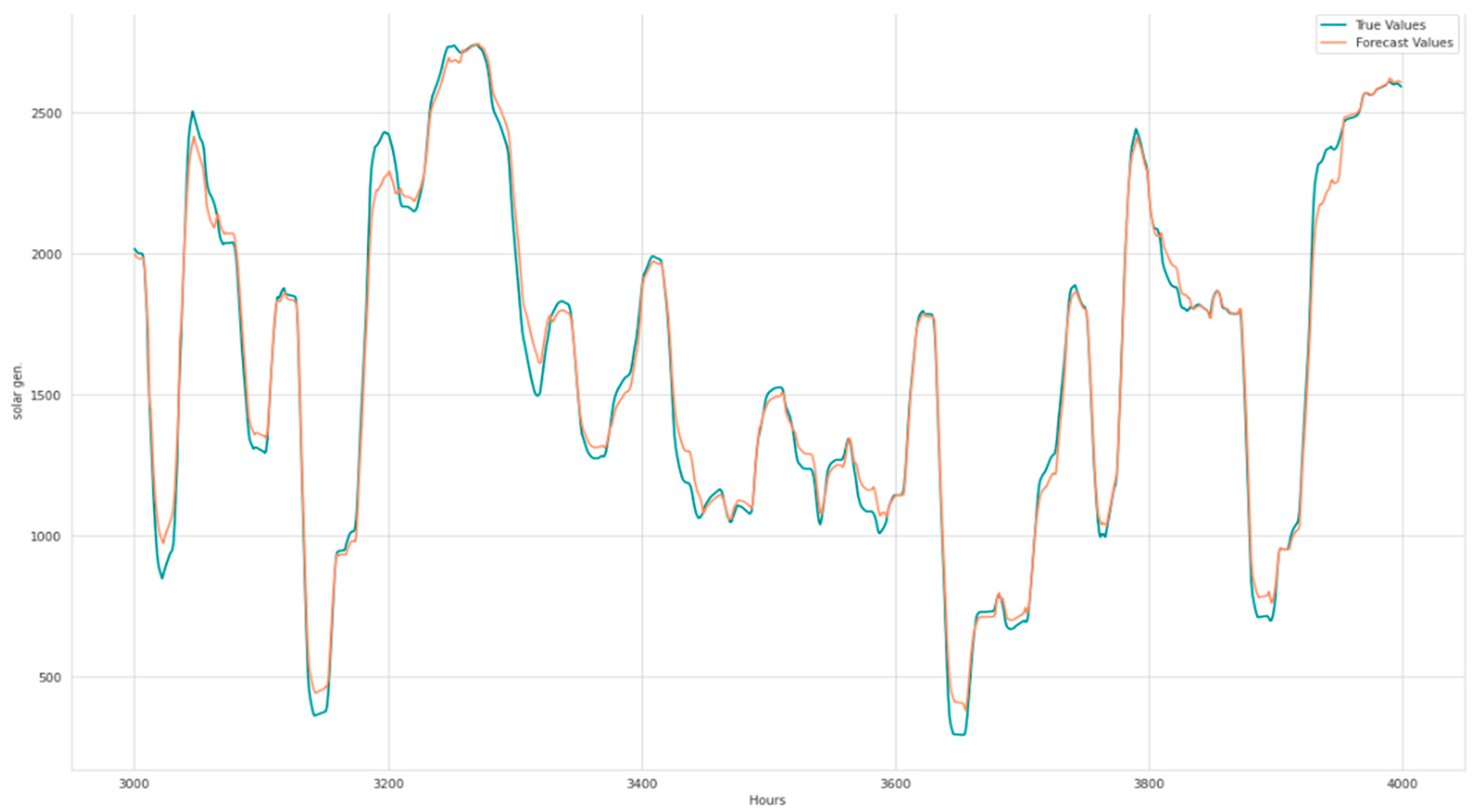
- ~15% and ~12% reductions in MASE, ~30% and ~33% reduction in test loss, for solar generation forecasting when paired with rainfall and temperature, respectively (Appendix A Table A2).
- ~12% reductions in MASE, ~6% and ~9% reductions in test loss, for wind generation combined with wind speed and all five variables, respectively (Appendix A Table A2).
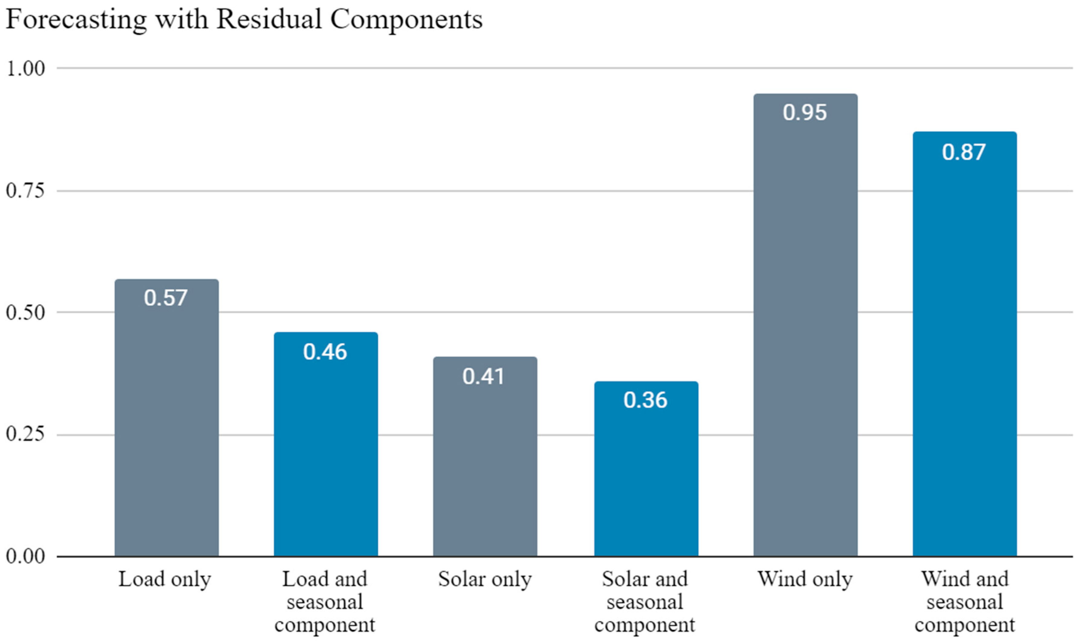
5. Seasonal Decomposition as a Source of Exogenous LSTM Input
- ~19% reduction in MASE and ~29% reduction in test loss for load forecasting.
- ~12% reduction in MASE and ~19% reduction in test loss for solar generation forecasting.
- ~8% reduction in MASE and test loss for wind generation forecasting.
- ~12% reduction in MASE and a ~31% reduction in test loss for solar generation forecast with the seasonal component and temperature, all normalised.
6. Conclusions
Author Contributions
Funding
Data Availability Statement
Conflicts of Interest
Appendix A

| Target Variable: Load | hd | lr (10−3) | Drop. | Opt. | Test Loss (10−3) | MASE | Bias (10−3) |
|---|---|---|---|---|---|---|---|
| Model 1 | 100 | 1 | 0.2 | Adam | 1.3 | 0.58 | −0.75 |
| Model 1, bi | 100 | 1 | 0.2 | RMSProp | 1.0 | 0.5 | −6.6 |
| Model 1, gc | 200 | 1 | 0.2 | Adam | 0.86 | 0.46 | 1.0 |
| Model 1, bi, gc | 100 | 1 | 0.5 | Adam | 1.2 | 0.53 | −7.6 |
| Model 1, gc, nl4 | 400 | 0.1 | 0.2 | RMSProp | 1.1 | 0.51 | −3.5 |
| Model 2 | 400 | 0.1 | 0.2 | Adam | 0.93 | 0.47 | −1.3 |
| Model 2, bi | 200 | 1 | 0.2 | Adam | 0.84 | 0.44 | −7.2 |
| Model 2, gc | 100 | 0.1 | 0.5 | Adam | 0.90 | 0.48 | 3.1 |
| Target Variable: Solar Generation | hd | lr (10−3) | drop. | opt. | Test loss (10−3) | MASE | bias (10−3) |
| Model 1 | 100 | 1 | 0.2 | Adam | 0.96 | 0.38 | −1.8 |
| Model 1, bi | 400 | 0.1 | 0.2 | RMSProp | 1.0 | 0.44 | −7.9 |
| Model 1, gc | 100 | 1 | 0.5 | Adam | 0.99 | 0.39 | −2.6 |
| Model 1, bi, gc | 100 | 1 | 0.5 | RMSProp | 1.0 | 0.44 | −12 |
| Model 1, gc, nl4 | 200 | 0.1 | 0.2 | RMSProp | 0.96 | 0.4 | −8.0 |
| Model 2 | 400 | 0.1 | 0.2 | Adam | 0.84 | 0.39 | 7.1 |
| Model 2, bi | 100 | 0.1 | 0.2 | RMSProp | 1.4 | 0.49 | −1.6 |
| Model 2, gc | 400 | 0.1 | 0.2 | Adam | 0.86 | 0.43 | 13 |
| Target Variable: Wind Generation | hd | lr (10−3) | Drop. | Opt. | Test Loss (10−3) | MASE | Bias (10−3) |
| Model 1 | 200 | 1 | 0.2 | Adam | 1.2 | 0.84 | −0.47 |
| Model 1, bi | 200 | 0.1 | 0.8 | RMSProp | 1.3 | 0.95 | 0.55 |
| Model 1, gc | 400 | 0.01 | 0.5 | Adam | 1.3 | 0.96 | 0.051 |
| Model 1, bi, gc | 200 | 0.1 | 0.8 | RMSProp | 1.3 | 0.95 | 1.1 |
| Model 1, gc, nl4 | 200 | 0.1 | 0.5 | RMSProp | 1.3 | 0.91 | −1.5 |
| Model 2 | 400 | 0.1 | 0.2 | RMSProp | 1.3 | 0.88 | −1.7 |
| Model 2, bi | 100 | 0.1 | 0.2 | RMSProp | 1.3 | 1.03 | −2.9 |
| Model 2, gc | 200 | 0.1 | 0.2 | RMSProp | 1.3 | 0.87 | −0.20 |
| Target Variable: Load | hd | lr (10−3) | Drop. | Opt. | Test Loss (10−3) | MASE | Bias (10−3) |
|---|---|---|---|---|---|---|---|
| Target only | 200 | 1 | 0.5 | RMSProp | 1.2 | 0.57 | 2.8 |
| Target and temperature | 200 | 1 | 0.2 | Adam | 1.1 | 0.51 | −0.55 |
| Target and rainfall in last hour | 200 | 1 | 0.2 | RMSProp | 1.2 | 0.55 | −7.6 |
| Target and humidity | 200 | 1 | 0.2 | RMSProp | 1.2 | 0.54 | −3.5 |
| Target and cloud cover | 200 | 1 | 0.5 | RMSProp | 1.2 | 0.54 | −8.1 |
| Target and wind speed | 400 | 1 | 0.2 | RMSProp | 1.1 | 0.53 | −7.0 |
| Target and all exogenous variables | 100 | 1 | 0.2 | Adam | 1.3 | 0.58 | 0.75 |
| Target Variable: Solar Generation | hd | lr (10−3) | Drop. | Opt. | Test Loss (10−3) | MASE | Bias (10−3) |
| Target only | 400 | 1.0 | 0.5 | RMSProp | 1.2 | 0.41 | −13 |
| Target and temperature | 100 | 1.0 | 0.2 | Adam | 0.80 | 0.36 | 1.9 |
| Target and rainfall in last hour | 200 | 0.10 | 0.2 | Adam | 0.89 | 0.35 | 1.7 |
| Target and humidity | 100 | 1.0 | 0.2 | RMSProp | 1.1 | 0.39 | −13 |
| Target and cloud cover | 100 | 1.0 | 0.2 | RMSProp | 1.2 | 0.40 | −14 |
| Target and wind speed * | 100 | 1.0 | 0.5 | RMSProp | 1.3 | 0.47 | −12 |
| Target and all exogenous variables | 100 | 1.0 | 0.2 | Adam | 0.96 | 0.38 | −1.8 |
| Target and all exogenous variables apart from wind | 100 | 1.0 | 0.2 | Adam | 0.99 | 0.39 | −4.9 |
| Target with temperature and rainfall | 100 | 1.0 | 0.2 | Adam | 0.93 | 0.38 | −2.4 |
| Target Variable: Wind Generation | hd | lr (10−3) | Drop. | Opt. | Test Loss (10−3) | MASE | Bias (10−3) |
| Target only | 100 | 1 | 0.2 | Adam | 1.3 | 0.95 | −7.7 |
| Target and temperature | 100 | 1 | 0.5 | Adam | 1.2 | 0.87 | 2.4 |
| Target and rainfall in last hour | 100 | 1 | 0.5 | RMSProp | 1.3 | 0.91 | −5.9 |
| Target and humidity * | 200 | 1 | 0.2 | Adam | 1.3 | 0.96 | −5.8 |
| Target and cloud cover | 200 | 1 | 0.2 | RMSProp | 1.4 | 0.97 | −9.3 |
| Target and wind speed | 100 | 1 | 0.2 | Adam | 1.2 | 0.84 | −4.3 |
| Target and all exogenous variables | 200 | 1 | 0.2 | Adam | 1.2 | 0.84 | −0.47 |
| Input Variables | hd | lr (10−3) | Drop. | opt. | Test loss (10−3) | MASE | Bias (10−3) |
|---|---|---|---|---|---|---|---|
| Load only | 200 | 1 | 0.5 | RMSProp | 1.2 | 0.57 | 2.8 |
| Load and seasonal component | 200 | 1 | 0.2 | Adam | 0.85 | 0.46 | 7.2 |
| Solar only | 400 | 1 | 0.5 | RMSProp | 1.2 | 0.41 | −13 |
| Solar and seasonal component | 200 | 0.1 | 0.2 | Adam | 0.97 | 0.36 | 0.12 |
| Wind only | 100 | 1 | 0.2 | Adam | 1.3 | 0.95 | −7.7 |
| Wind and seasonal component | 100 | 1 | 0.2 | Adam | 1.2 | 0.87 | −6.5 |


References
- Mbuli, N.; Mathonsi, M.; Seitshiro, M.; Pretorius, J.H.C. Decomposition forecasting methods: A review of applications in power systems. Energy Rep. 2020, 6, 298–306. [Google Scholar] [CrossRef]
- Dudek, G. Pattern-based local linear regression models for short-term load forecasting. Electr. Power Syst. Res. 2016, 130, 139–147. [Google Scholar] [CrossRef]
- Ariyo, A.A.; Adewumi, A.O.; Ayo, C.K. Stock Price Prediction Using the ARIMA Model. In Proceedings of the 2014 UK Sim-AMSS 16th International Conference on Computer Modelling and Simulation, Cambridge, UK, 26–28 March 2014; pp. 106–112. [Google Scholar] [CrossRef]
- Wang, Y.; Sun, S.; Chen, X.; Zeng, X.; Kong, Y.; Chen, J.; Guo, Y.; Wang, T. Short-term load forecasting of industrial customers based on SVMD and XGBoost. Int. J. Electr. Power Energy Syst. 2021, 129, 106830. [Google Scholar] [CrossRef]
- Elsaraiti, M.; Merabet, A. A Comparative Analysis of the ARIMA and LSTM Predictive Models and Their Effectiveness for Predicting Wind Speed. Energies 2021, 14, 6782. [Google Scholar] [CrossRef]
- Tarmanini, C.; Sarma, N.; Gezegin, C.; Ozgonenel, O. Short term load forecasting based on ARIMA and ANN approaches. Energy Rep. 2023, 9 (Suppl. S3), 550–557. [Google Scholar] [CrossRef]
- Markovics, D.; Mayer, M.J. Comparison of machine learning methods for photovoltaic power forecasting based on numerical weather prediction. Renew. Sustain. Energy Rev. 2022, 161, 112364. [Google Scholar] [CrossRef]
- Rodríguez, F.; Fleetwood, A.; Galarza, A.; Fontán, L. Predicting solar energy generation through artificial neural networks using weather forecasts for microgrid control. Renew. Energy 2018, 126, 855–864. [Google Scholar] [CrossRef]
- Wang, L.; Mao, M.; Xie, J.; Liao, Z.; Zhang, H.; Li, H. Accurate solar PV power prediction interval method based on frequency-domain decomposition and LSTM model. Energy 2023, 262, 125592. [Google Scholar] [CrossRef]
- Elman, J.L. Finding structure in time. Cogn. Sci. 1990, 14, 179–211. [Google Scholar] [CrossRef]
- Hochreiter, S.; Schmidhuber, J. Long short-term memory. Neural Comput. 1997, 9, 1735–1780. [Google Scholar] [CrossRef]
- Lu, S.; Zhu, Y.; Zhang, W.; Wang, J.; Yu, Y. Neural Text Generation: Past, Present and Beyond. arXiv 2018, arXiv:1803.07133. [Google Scholar]
- Elsaraiti, M.; Merabet, A. Solar Power Forecasting Using Deep Learning Techniques. IEEE Access 2022, 10, 31692–31698. [Google Scholar] [CrossRef]
- Memarzadeh, G.; Keynia, F. A new short-term wind speed forecasting method based on fine-tuned LSTM neural network and optimal input sets. Energy Convers. Manag. 2020, 213, 112824. [Google Scholar] [CrossRef]
- Torres, J.; Martínez-Álvarez, F.; Troncoso, A. A deep LSTM network for the Spanish electricity consumption forecasting. Neural Comput. Appl. 2022, 34, 10533–10545. [Google Scholar] [CrossRef] [PubMed]
- Akhtar, S.; Shahzad, S.; Zaheer, A.; Ullah, H.S.; Kilic, H.; Gono, R.; Jasiński, M.; Leonowicz, Z. Short-Term Load Forecasting Models: A Review of Challenges, Progress, and the Road Ahead. Energies 2023, 16, 4060. [Google Scholar] [CrossRef]
- Ding, S.; Zhang, H.; Tao, Z.; Li, R. Integrating data decomposition and machine learning methods: An empirical proposition and analysis for renewable energy generation forecasting. Expert Syst. Appl. 2022, 204, 117635. [Google Scholar] [CrossRef]
- Kwon, B.-S.; Park, R.-J.; Song, K.-B. Short-Term Load Forecasting Based on Deep Neural Networks Using LSTM Layer. J. Electr. Eng. Technol. 2020, 15, 1501–1509. [Google Scholar] [CrossRef]
- Machado, E.; Pinto, T.; Guedes, V.; Morais, H. Electrical Load Demand Forecasting Using Feed-Forward Neural Networks. Energies 2021, 14, 7644. [Google Scholar] [CrossRef]
- Wojtkiewicz, J.; Hosseini, M.; Gottumukkala, R.; Chambers, T.L. Hour-Ahead Solar Irradiance Forecasting Using Multivariate Gated Recurrent Units. Energies 2019, 12, 4055. [Google Scholar] [CrossRef]
- Xie, A.; Yang, H.; Chen, J.; Sheng, L.; Zhang, Q. A Short-Term Wind Speed Forecasting Model Based on a Multi-Variable Long Short-Term Memory Network. Atmosphere 2021, 12, 651. [Google Scholar] [CrossRef]
- Jhana, N. Hourly Energy Demand Generation and Weather. Available online: https://www.kaggle.com/datasets/nicholasjhana/energy-consumption-generation-prices-and-weather (accessed on 12 July 2023).
- ENTSO-E. Transparency Platform 2019. Available online: https://transparency.entsoe.eu/dashboard/show (accessed on 12 July 2023).
- OpenWeather API. 2019. Available online: https://openweathermap.org/api (accessed on 12 July 2023).
- Lin, J.; Ma, J.; Zhu, J.; Cui, Y. Short-term load forecasting based on LSTM networks considering attention mechanism. Int. J. Electr. Power Energy Syst. 2021, 137, 107818. [Google Scholar] [CrossRef]
- Abdel-Nasser, M.; Mahmoud, K. Accurate photovoltaic power forecasting models using deep LSTM-RNN. Neural Comput. Appl. 2019, 31, 2727–2740. [Google Scholar] [CrossRef]
- Mellit, A.; Pavan, A.M.; Lughi, V. Deep learning neural networks for short-term photovoltaic power forecasting. Renew Energy 2021, 172, 276–288. [Google Scholar] [CrossRef]
- Glorot, X.; Bengio, Y. Understanding the difficulty of training deep feedforward neural networks. In Proceedings of the Thirteenth International Conference on Artificial Intelligence and Statistics, Sardinia, Italy, 13–15 May 2010; pp. 249–256. [Google Scholar]
- Statsmodel Documentation for the Seasonal_Decompose Function. Available online: https://www.statsmodels.org/dev/generated/statsmodels.tsa.seasonal.seasonal_decompose.html (accessed on 20 August 2023).
- Hyndman, R.J.; Koehler, A.B. Another look at measures of forecast accuracy. Int. J. Forecast. 2006, 22, 679–688. [Google Scholar] [CrossRef]
- Kingma, D.P.; Ba, J. Adam: A method for stochastic optimization. arXiv 2014, arXiv:1412.6980. [Google Scholar]
- Hinton, G. Coursera Neural Networks for Machine Learning, Lecture 6. 2018. Available online: https://www.cs.toronto.edu/~tijmen/csc321/slides/lecture_slides_lec6.pdf (accessed on 29 January 2024).
- Sachdeva, A.; Jethwani, G.; Manjunath, C.; Balamurugan, M.; Krishna, A.V.N. An Effective Time Series Analysis for Equity Market Prediction Using Deep Learning Model. In Proceedings of the International Conference on Data Science and Communication (IconDSC), Bangalore, India, 1–2 March 2019; pp. 1–5. [Google Scholar] [CrossRef]
- Ruder, S. An overview of gradient descent optimization algorithms. arXiv 2016, arXiv:1609.04747. [Google Scholar]
- Schuster, M.; Paliwal, K.K. Bidirectional recurrent neural networks. IEEE Trans. Signal Process. 1997, 45, 2673–2681. [Google Scholar] [CrossRef]
- Ko, M.-S.; Lee, K.; Kim, J.-K.; Hong, C.W.; Dong, Z.Y.; Hur, K. Deep Concatenated Residual Network With Bidirectional LSTM for One-Hour-Ahead Wind Power Forecasting. IEEE Trans. Sustain. Energy 2021, 12, 1321–1335. [Google Scholar] [CrossRef]
- Pascanu, R.; Mikolov, T.; Bengio, Y. On the difficulty of training recurrent neural networks. In Proceedings of the International Conference on Machine Learning, Atlanta, GA, USA, 7–19 June 2013; Volume 28, pp. 1310–1318. [Google Scholar]
- Bengio, Y.; Courville, A.; Vincent, P. Representation Learning: A Review and New Perspectives. IEEE Trans. Pattern Anal. Mach. Intell. 2013, 35, 1798–1828. [Google Scholar] [CrossRef]
- Lim, S.C.; Huh, J.H.; Hong, S.K.; Park, C.Y.; Kim, J.C. Solar Power Forecasting Using CNN-LSTM Hybrid Model. Energies 2022, 15, 8233. [Google Scholar] [CrossRef]
- Ribeiro, M.H.D.M.; da Silva, R.G.; Ribeiro, G.T.; Mariani, V.C.; Coelho, L.S. Cooperative ensemble learning model improves electric short-term load forecasting. Chaos Solitons Fractals 2023, 166, 112982. [Google Scholar] [CrossRef]


| Hyperparameter | Variation 1 | Variation 2 | Variation 3 |
|---|---|---|---|
| Hidden Layer Dimension | 100 | 200 | 400 |
| Learning Rate | 1.0 × 10⁻³ | 1.0 × 10⁻⁴ | 1.0 × 10⁻⁵ |
| Dropout Probability | 0.2 | 0.5 | 0.8 |
| Optimiser Algorithm | Adam | RMSProp | SGD |
Disclaimer/Publisher’s Note: The statements, opinions and data contained in all publications are solely those of the individual author(s) and contributor(s) and not of MDPI and/or the editor(s). MDPI and/or the editor(s) disclaim responsibility for any injury to people or property resulting from any ideas, methods, instructions or products referred to in the content. |
© 2024 by the authors. Licensee MDPI, Basel, Switzerland. This article is an open access article distributed under the terms and conditions of the Creative Commons Attribution (CC BY) license (https://creativecommons.org/licenses/by/4.0/).
Share and Cite
Shering, T.; Alonso, E.; Apostolopoulou, D. Investigation of Load, Solar and Wind Generation as Target Variables in LSTM Time Series Forecasting, Using Exogenous Weather Variables. Energies 2024, 17, 1827. https://doi.org/10.3390/en17081827
Shering T, Alonso E, Apostolopoulou D. Investigation of Load, Solar and Wind Generation as Target Variables in LSTM Time Series Forecasting, Using Exogenous Weather Variables. Energies. 2024; 17(8):1827. https://doi.org/10.3390/en17081827
Chicago/Turabian StyleShering, Thomas, Eduardo Alonso, and Dimitra Apostolopoulou. 2024. "Investigation of Load, Solar and Wind Generation as Target Variables in LSTM Time Series Forecasting, Using Exogenous Weather Variables" Energies 17, no. 8: 1827. https://doi.org/10.3390/en17081827
APA StyleShering, T., Alonso, E., & Apostolopoulou, D. (2024). Investigation of Load, Solar and Wind Generation as Target Variables in LSTM Time Series Forecasting, Using Exogenous Weather Variables. Energies, 17(8), 1827. https://doi.org/10.3390/en17081827