Abstract
This study proposes a novel double closed-loop robust control strategy based on a power switching affine model of three-phase voltage source converters (VSCs). The aim is to overcome the challenges posed by inaccurate mathematical models, complex controller configurations, indirect switching control, and performance degradation under circuit parameters uncertainty or load variation in conventional methods. These conventional methods rely on linearization models, duty ratio regulation, and pulse width modulation (PWM) technologies. The contributions of work are the following: (1) A two-dimensional (2D) power switching affine model is constructed without any approximation or averaging. (2) The proposed approach achieves direct switching control of three-phase VSCs, eliminating the need for complex rotation coordinate transformation, PWM, and phase locking loop (PLL), which are utilized in traditional control methods. (3) The rigor of the system stability analysis is enhanced based on the 2D power switching model compared to the existing three-dimensional (3D) current switching model. (4) A simple control structure with only two control parameters is employed to address circuit parameter uncertainties. The effectiveness and superiority of the proposed method is validated through simulation and experimental comparison results.
1. Introduction
Three-phase voltage source converters (VSCs) are extensively used in renewable energy systems, electric mobility, and decentralized power generation, among other applications [1,2,3]. The operation of these converters depends on the discrete switching states of power switches, making three-phase VSCs inherently nonlinear systems. The conventional linearized modeling methods of converters, such as the commonly employed small signal modeling techniques [4,5], are derived by disregarding high-frequency components of system states and averaging them over a switching period. Therefore, they fail to accurately depict the operational procedures of three-phase VSCs [6], thereby impeding the design of high-performance controllers.
The conventional control approaches for three-phase VSCs, such as the traditional voltage-oriented control (VOC) methods [7] and direct power control (DPC) methods [8], rely heavily on linearized models. However, these methods suffer from the drawbacks of intricate controller design and challenges in tuning control parameters. On one hand, the rotation coordinate transformations are commonly employed within traditional controller design frameworks to convert the three-phase AC states into two-phase DC states, i.e., the direct- and quadrature-axis components [7,8]. To regulate the direct- and quadrature-axis components effectively, it is necessary to employ multiple control loops and decoupled control technology. However, uncertainties in circuit parameters inevitably lead to performance degradation within this control framework [9,10,11,12,13,14]. Sliding mode control (SMC) [9], adaptive control [10], and fuzzy control [11] are integrated with traditional VOC or DPC methods to enhance system robustness against uncertainties in circuit parameters or variations in load. Yet, these approaches introduce new challenges, such as the controller output chattering in SMC [12], difficulty in selecting appropriate parameters for adaptive control [13], and real-time control issues in fuzzy control [14]. On the other hand, duty ratio regulation is commonly employed for three-phase VSCs due to the reliance of traditional controller design on linearization models. This necessitates the utilization of complex pulse width modulation (PWM) technology [15,16]. However, the range within which system states can be regulated may be limited due to constraints on modulation ratio variation in PWM [16].
The model predictive control (MPC) methods have recently gained significant attention due to their ability to address the aforementioned issues in VOC and DPC. By minimizing the cost function based on predictive errors of system states, MPC methods allow for the regulation of multiple system states within a single control loop and facilitate direct selection of switching states for three-phase VSCs in the next control cycle [17,18]. However, uncertainties in circuit parameters can cause inaccuracies in the predictive values. Therefore, it is necessary to employ extended observers or compensators to enhance the control performance of MPC when dealing with circuit parameter uncertainties [19,20]. This necessitates addressing complexities associated with observer design and additional parameter tuning issues. Moreover, the selection of multi-objective weights and conducting stability analysis for MPC pose ongoing challenges [21].
The theory of switching systems offers a novel solution for addressing the issues encountered in traditional converter modeling and control methods. The three-phase VSCs, operating at different switching states, can be considered as distinct subsystems. In [22,23], the discrete-time switching linear model is constructed for three-phase active power filter (APF). Then, a quadratic linear optimal controller and an H∞ controller are designed to regulate the AC current. The switching models presented in [22,23] accurately capture the switching characteristics of the three-phase APF. However, it should be noted that the linearized process of the model in [22,23] still falls within the scope of duty radio control and therefore cannot be expected to facilitate system analysis. The switching affine models in [24,25,26] are constructed for the three-phase AC-DC converter. In contrast to traditional linearization models, these switching affine models in [24,25,26] are built without linearization. Thus, they achieve an accurate description of the working process of the converter. Moreover, by designing a stability-based switching rule in [24,25,26], the converter achieves regulation of its AC current directly through subsystem switching. The need for complex rotation coordinate transformations and PWM processes in conventional control methods is avoided. In [27], a switching model is developed for unbalanced grid based on the positive- and negative-sequence current components of the three-phase PWM converter. It is emphasized in [27] that this switching rule possesses the important characteristic of being insensitive to circuit parameters. Therefore, compared to traditional VOC, DPC, and MPC methods, the utilization of the switching control method [27] enables achieving strong system robustness without requiring additional observers or compensation blocks. However, despite the research accomplishments presented in [24,25,26,27], there are still two areas that require further improvement.
Firstly, existing methods based on switching system theory in [22,23,24,25,26,27] for three-phase VSCs primarily focus on the states of three-phase AC current. These methods typically involve formulating three-dimensional (3D) current switching affine models [26,27]. Due to the different equilibrium points of various subsystems in a switching affine model, system stability analysis and switching controller design commonly rely on the ‘average’ model and common Lyapunov function (CLF) [28,29]. In other words, an ‘average’ model of system under a specific switching sequence is established by addressing a convex combination of multiple subsystems. Subsequently, the asymptotic or quadratic stability of this ‘average’ system with an equilibrium at the origin is analyzed based on CLF. However, the traditional 3D current switching affine model in [26,27] faces a problem of solving four equations to find three convex combination variables when considering the combinations of three subsystems. A unique solution becomes unattainable. For this problem, in [26,27], one among the three current states has to be disregarded to reduce formula dimensionality. Although the authors of [26,27] argue for the formula’s reasonableness under three-phase balanced conditions, issues of inaccurate representation persist. Additionally, achieving strict grid balance conditions is challenging in real-world applications; hence, traditional stability analysis based on current switching models is not rigorous enough.
Secondly, the dynamic behavior of the overall control system is limited by that of the outer control loop in the commonly used double closed-loop controller for three-phase VSCs, where the reference for the inner loop controller is derived from the output of the outer loop controller. Therefore, although it has been demonstrated in [27] that the switching control in inner loop exhibits insensitivity to circuit parameters, further enhancements are still required to improve the robustness of the outer loop controller against load variations.
To address the aforementioned issues in traditional control methods and existing switching control methods based on the 3D current switching model, this paper proposes a robust control strategy for three-phase VSCs. The strategy is based on a two-dimensional (2D) power switching affine model to handle uncertainties in AC-side inductance and circuit equivalent resistance, as well as load variations. The proposed control system comprises an inner loop power switching controller and an outer loop feedback linearization controller with sliding mode observer (SMO). The proposed method offers several key advantages: (1) A controller configuration with only two control parameters is employed, which is characterized by its simplicity. (2) It achieves high-performance control of the system, even in the presence of uncertainties in circuit parameters and variations in load.
2. Power Switching Affine Model
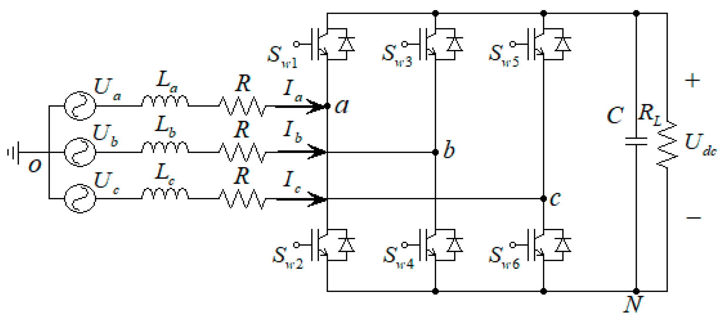
The circuit diagram of three-phase VSCs is illustrated in Figure 1. ua, ub, uc, ia, ib, and ic represent the three-phase AC voltages and currents, respectively. The AC-side filter inductance is La = Lb = Lc = L. R signifies the circuit equivalent resistance. Swi (i = 1, …, 6) are the switching devices. The DC-side filter capacitor is C and load is RL. Udc indicates the DC voltage.
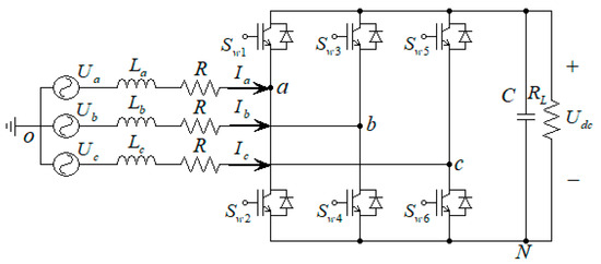
Figure 1.
Three-phase VSCs circuit.
According to the instantaneous power theory in [30], the instantaneous active and reactive power P(t) and Q(t) of three-phase VSCs are defined as
where uα(t) = (2ua(t) − ub(t) − uc(t))/3, , iα(t) = (2ia(t) − ib(t) − ic(t))/3, denote the AC voltage and current components under two-phase static (αβ) coordinate frames, respectively.
The primary control objectives for three-phase VSCs in Figure 1 encompass regulating the DC voltage Udc and synchronizing the three-phase AC voltages and currents [7]. These control objectives can be equivalent to the instantaneous power control of P(t) and Q(t) [8]. Defining system power references are Pr and Qr; then, we have system state error vector , where and . By calculating the derivative of (1) by substituting the traditional current differential equations of three-phase VSCs in [7], we can express a power switching affine error model as
where ω = 2πf is angle frequency of AC voltages; f is AC voltage frequency; A is state matrix; bσ is switching affine item, where is switching signal; m is the number of subsystems; Fα and Fβ are discrete switching functions, defined as
where and are discrete switching components under αβ coordinate frames, respectively; Swj (j = a, b, c) is discrete switching states of j bridge lags in Figure 1, where Swj = 1 presents the upper switch of j-leg in Figure 1 is turned ON and the bottom switch is turned OFF; Swj = 0 has contrary situation. It is evident that the three-phase VSCs consist of m = 8 subsystems, as per Suσ = [Fα Fβ] = [Swa Swb Swc] (σ ∈ {1, …, m}), as shown in Table 1.

Table 1.
The subsystems definitions.
The power switching affine model, denoted as model (2), stands out from the traditional linearization models in [4,5,6,7] by simultaneously describing the continuous dynamics of subsystems’ instantaneous power and the discrete switching process of the converter. This model accurately captures the operational dynamics of three-phase VSCs. In contrast to the conventional 3D current switching models in [24,25,26,27], the power switching model (2) adopts a 2D representation. This characteristic offers significant advantages in terms of system stability analysis and design of switching rules, which will be further discussed.
3. Proposed Controllers Design
3.1. Inner Loop Switching Controller
Under the switching theory frameworks, the switching rule is designed to select the switching signal σ, where the system asymptotic or quadratic stability should be guaranteed. The following Theorem 1, which considers the stability and switching rule simultaneously, is proposed.
If a convex combination vector λ, which satisfies the following condition, exists
Theorem 1.
For the switching affine model (2) of three-phase VSCs with N subsystems (N < m). If there exists a convex combination vector that satisfies the following condition
Then, is asymptotical stable equilibrium point under the switching rule
Proof of Theorem 1.
The following ‘average’ model of switching system (2) is considered based on the convex combination of subsystems [27,28,29].
where , and . It is clear that the equilibrium points of system (6) depend on the affine item . Defining a CLF, expressed as
where D = diag{d d} is a positive definite symmetric matrix and thus . By calculating the derivative of (7), we have
Due to and is Hurwitz, we have
Thus, according to Theorem 1, if a convex combination vector exists and satisfies for (8), then is satisfied, i.e., the asymptotical stable of (6) to original point is guaranteed. For the switching system (2), the behavior of the ‘average’ model can be mimicked by means of fast switching between the different subsystems with correct proportion of time (σ = 1, …, N) on each constant time interval. According to [24,25,26,27,28,29], the state-dependent switching rule, where the subsystem has minimum is selected for the next cycle, is defined by
From Equations (2), (8), and (10), the subsystem leads to minimum is equal to the subsystem has minimum value of item in (8), which is
The first term on the right side of Equation (11) is identical for all subsystems. Therefore, the relative value of each subsystem is determined by the second term on the right side of Equation (11). As a result, the switching rule can be simplified as (5). □
Remark 1.
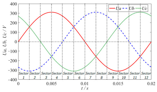
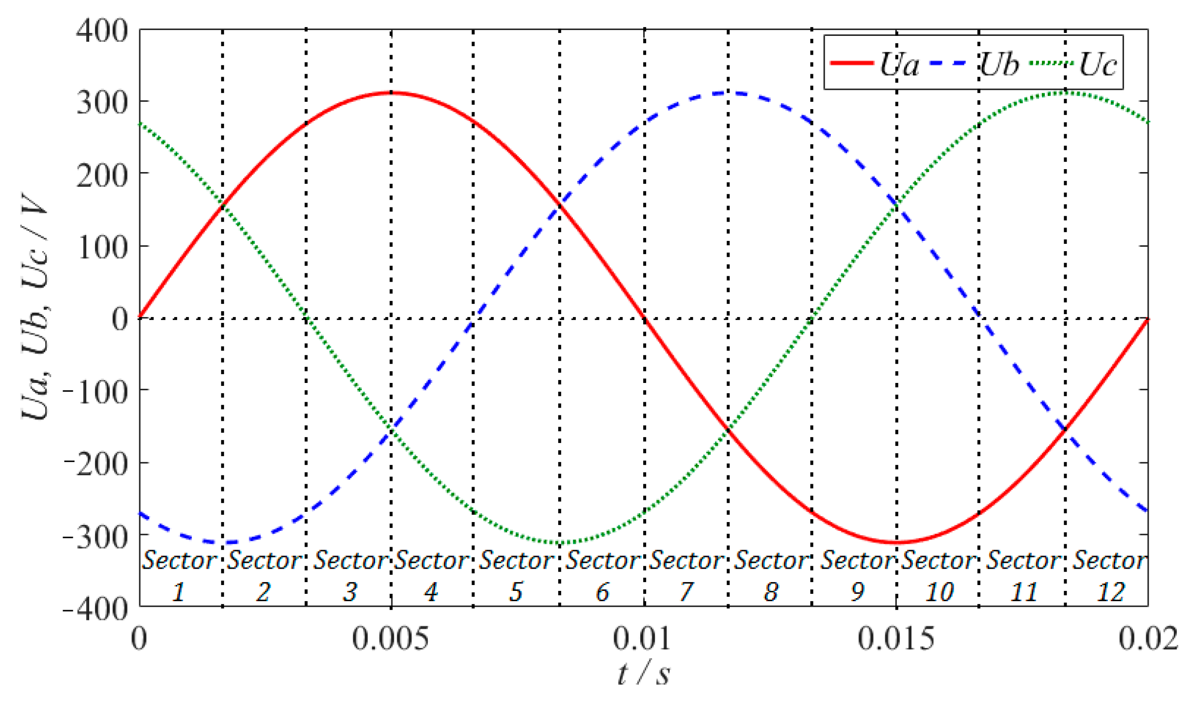
The necessary stability condition for switching system (2) with multiple equilibria, as stated in Theorem 1, is the existence of an ‘average’ model with an equilibrium at the origin. Therefore, it is crucial to confirm the number of subsystems N mentioned in Theorem 1. Since the proposed power switching model involves 2 state variables, it is required that the number of convex combination variables N should be 3 to ensure solvability of Equation (4). Similar to [25,26,27], we employ sector division and minimum switching principle to obtain a subset of switching signals for constructing an ‘average’ model. In this paper, we divide an AC voltage period into 12 sectors, as illustrated in Figure 2. In each sector, only the switching stability between 3 out of 8 subsystems needs to be considered. Using sector 2 for instance, because ub < 0 and its absolute value is bigger than voltage ua and uc, the bottom switch of b leg in Figure 1 should be turned ON according the working principle of three-phase VSCs, i.e., Swb = 0. Thus, only the subset of subsystems Su1, Su2, Su5, and Su6 in Table 1 are feasible in sector 2. Furthermore, in accordance with the principle of minimum switching, it is imperative to minimize the interchanging of bridge legs in converter as a means to mitigate switching losses. The switching between subsystems Su2 = [Swa Swb Swc] = [0 0 1] and Su5 = [Swa Swb Swc] = [1 0 0] should be avoided in sector 2. Consequently, in sector 2, a subset of subsystems (Su1, Su2, Su6) and a subset of subsystems (Su1, Su5, Su6) should be considered according to Theorem 1. The stability for subset of subsystems (Su1, Su5, Su6) and (Su1, Su2, Su6) are analyzed separately according to Theorem 1.
Figure 2.
Twelve-sector division of the three-phase VSCs.
For the subset of subsystems (Su1, Su5, Su6), if subsystems Su1, Su5, or Su6 are activated, respectively, we have
According to Theorem 1, if there exist (n = 1, 2, 3) satisfying the following equations, then the switching stability of three-phase VSCs in sector 2 can be guaranteed.
By solving (13), we obtain
Due to uα > 0 > uβ in sector 2, λ1 to λ3 in (14) satisfy the stability conditions of Theorem 1. Thus, the switching between subsystems Su1, Su5, and Su6 is feasible in sector 2. In contrary, for the subset of subsystems (Su1, Su2, and Su6), we have
The infeasibility of switching between subsystems Su1, Su2, and Su6 in sector 2 is attributed to the negative value of λ2, as indicated by Equation (15). As a result, an offline system stability analysis can be conducted for all 12 sectors depicted in Figure 2, followed by the construction of an offline switching Table 2. For each sampling period, the switching states of three-phase VSCs for the next control cycle can be directly selected from the offline switching table, shown in Table 2, based on the switching rule (5).
Table 2.
Offline switching table.
Remark 2.
The sector division approach adopted in this work is similar to the methods utilized in [25,26,27]. However, due to the utilization of a 2D power switching model, the stability analysis becomes more rigorous. When analyzing system stability for N = 3 subsystems across different sectors in the traditional 3D current switching model discussed in [26,27], four equations need to be solved to determine three convex combination variables. It is not possible to obtain a unique solution. In [26,27], one of the three current variables in the traditional current switching model is disregarded to reduce formula dimensions. The authors of [26,27] argue that this practice is reasonable under balanced grid conditions. However, it is inappropriate both in terms of formula expression and actual system operating conditions. If one of the three current variables is ignored in these traditional models, it becomes difficult to claim that an accurate ‘average’ model of the switching system has been obtained. Additionally, it is challenging to achieve strict balance in converter grids in real-world applications. Therefore, the stability conditions may not be rigorous for three-phase VSCs based on traditional 3D current switching models. In contrast, the proposed 2D power switching model for system stability analysis overcomes these limitations.
Remark 3.
Compared to the traditional control method of three-phase VSCs, the proposed inner loop switching control method offers a simpler control system configuration without any control parameters. Additionally, the proposed switching rule (5) demonstrates robustness against circuit parameter uncertainty due to its insensitivity towards the circuit parameters L and R in model (2). Furthermore, in comparison to the traditional switching rule (10) and the switching rule utilized in [25,26,27] based on the conventional current switching model, the proposed power-based switching rule (5) is further simplified, rendering it more suitable for digital programming.
3.2. Outer Loop Feedback Linearization Controller with Sliding Mode Observer
To ensure the constant DC voltage control objectives of three-phase VSCs, the outer loop controller should be robust to load variations in accordance with changing working conditions. In other words, since the active power reference Pr in inner control loop is determined by the outer loop controller, it is essential for the outer loop control to be robust against load variations and calculate the power reference Pr based on the real-time load of the converter. In this subsection, we extend our previous work [31] by combining an outer loop feedback linearization controller with SMO with the inner loop switching controller.
The voltage equation of three-phase VSCs under two-phase (dq) rotation coordinate frame is given by [7,31]
where is manipulating variable; Swd is active-axis component of switching states Swj (j = a, b, c); idr is the current reference of active-axis current id; iL is load current. Assuming the DC voltage reference is Udcr and the DC voltage state error is eu = Udc − Udcr, the conventional feedback linearization control law in [32] can be used, given by
where ku > 0 is the control gain. However, the load may vary according to the working conditions, i.e., the DC current iL = Udc/RL is the variation. Therefore, the active power reference Pr = iLUdcr may inaccurate under load variations. A SMO is used for the current estimation of load, as expressed in Theorem 2.
Theorem 2.
For three-phase VSCs voltage Equation (17), if the following feedback linearization control law with the SMO are used for outer control loop
where is the improved manipulated variable; is an estimated load current; is estimation value of DC voltage; is the sliding mode item and γ is the observer gain; is the estimate error of DC voltage. Then, the DC voltage tracking control can be achieved. Meanwhile, the observing error ev of DC voltage and observing error of load current approach to zero exponentially.
Proof of Theorem 2.
Due to the minimal DC voltage fluctuation in three-phase VSCs at high switching frequencies, it can be assumed that there is no load current fluctuation, i.e., . Therefore, the output DC voltage and current states are expressed as
Using (20) minus (19), we have
Defining the Lyapunov function
Then, the derivative of (22) is
The observing error of DC voltage ev and the estimate error of load current eL converge exponentially to zero. Then, if the feedback linearization control law (18) is used for (19), we have . It is obvious that, as long as control gain ku > 0, the asymptotical stable of system is guaranteed. □
To this end, the active power reference is obtained, which is time-changing according to the load variation.
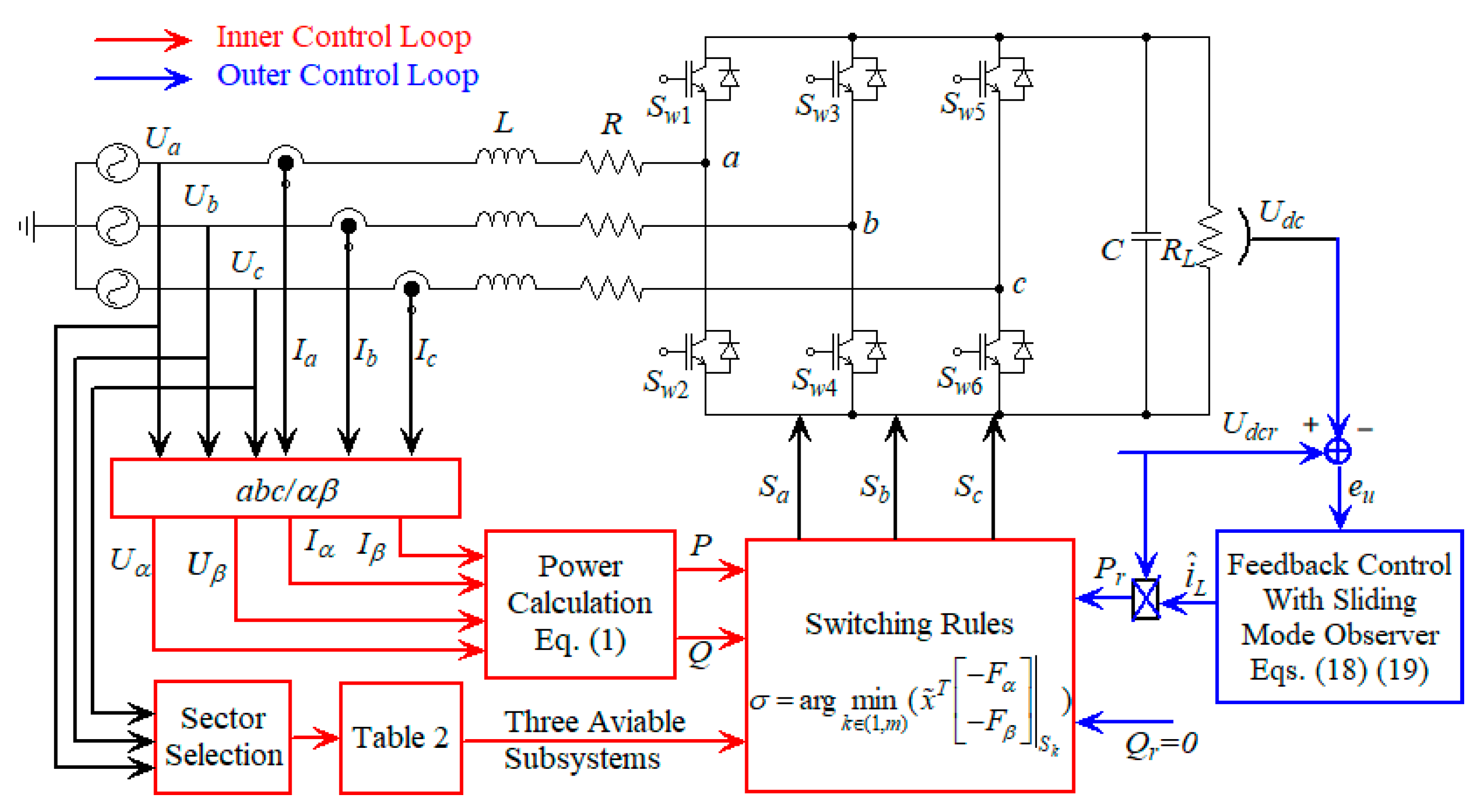
It is notable that the control law with SMO in Theorem 2 is derived based on the voltage Equation (16) under a two-phase rotating coordinate frame. However, the computation of control law (18) and SMO (19) does not require complex coordinate transformations at all. In conjunction with the inner loop controller, the complete control system of the proposed method can be designed within a two-phase static (αβ) coordinate frame. This approach eliminates the need for complex phase-locked loops (PLL) [33], coordinate transformations, and PWM processes commonly encountered in conventional control methods [7,8,9,10,11,12,13]. Moreover, only two positive control parameters (γ, ku) need adjustment in the proposed controller, which is very easy to choose based on control theory and simulation testing. To sum up, the block diagram of proposed methodology for three-phase VSCs is illustrated in Figure 3.

Figure 3.
The block diagram of proposed control method.
4. Simulation and Experimental Results
4.1. Simulation Results
The simulation model is built in Matlab 2018a using the nominal parameters given in Table 3.
Table 3.
Nominal parameters.
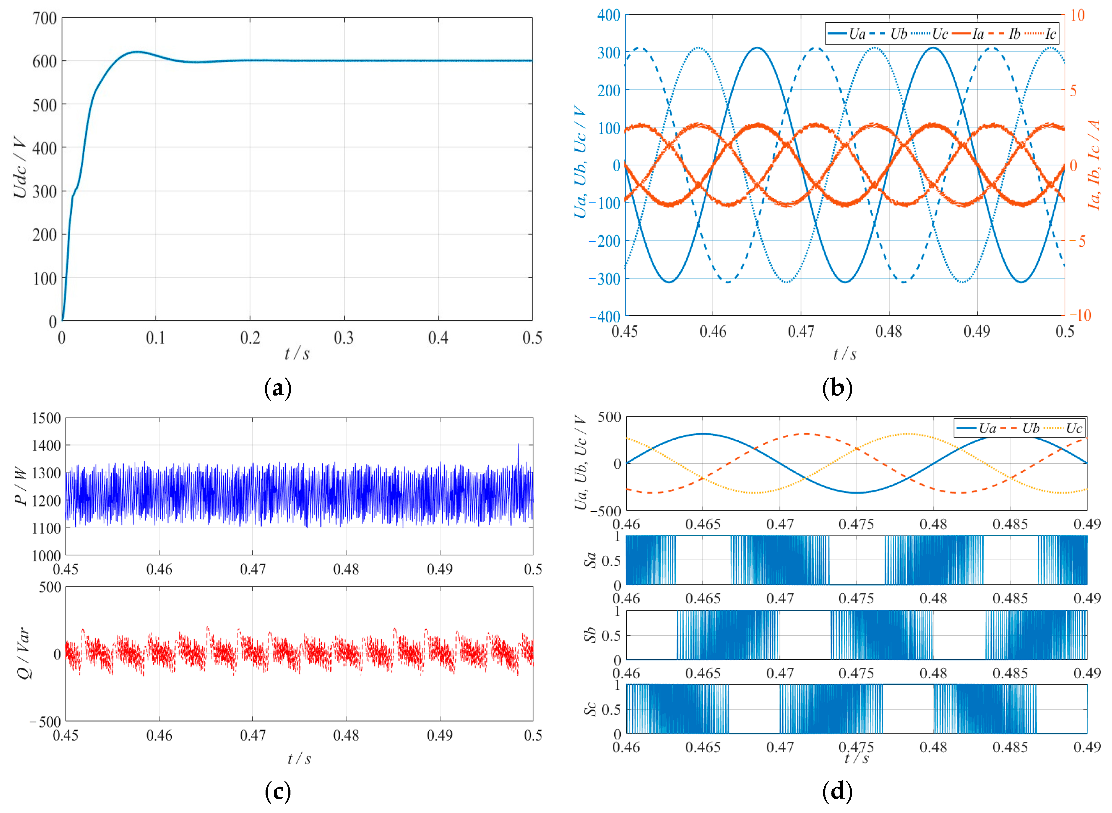
The simulation results of the proposed method for three-phase VSCs under nominal circuit parameters condition are illustrated in Figure 4. Specifically, Figure 4a displays the output DC voltage waveform, while Figure 4b presents the waveforms of three-phase voltage and current. Additionally, Figure 4c presents the active and reactive power waveforms and Figure 4d exhibits the switching states under switching control framework. From Figure 4a,c, the regulation of active power P leads to the control of DC voltage, where both of them reach the expected values. In Figure 4b,c, the regulation of reactive power Q to its expected value, Qr = 0, ensures that the input current is sinusoidal and synchronized with the input voltage, achieving high power factor control (PF = 0.9985). Moreover, according to distinct sector-based switching rules, the subsystem is selected directly using the proposed method for the next control cycle. Thus, during each control instant, one of the three bridge legs remains fixed for three-phase VSCs in Figure 4d, distinguishing it from conventional SPWM and SVPWM methods.
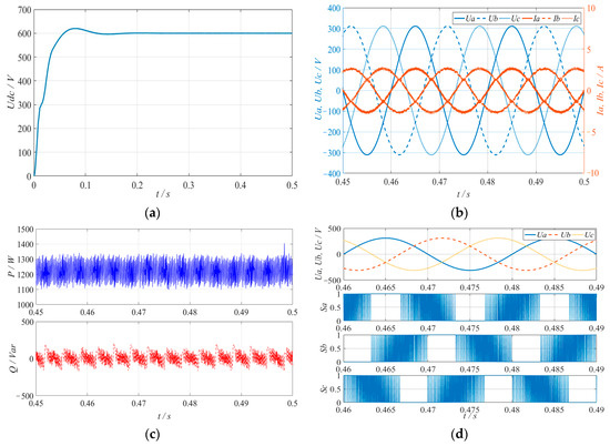
Figure 4.
Simulation results using proposed method with nominal parameters in Table 3: (a) output DC voltage waveform; (b) three-phase voltage and current waveforms; (c) the active and reactive power waveforms; (d) the three-phase bridge legs switching states.
The uncertainties of circuit parameters L and R, where the estimated values = 20 mH and = 1 Ω are utilized in inner loop controller and the actual circuit parameters remain the nominal values in Table 3, have been taken into consideration. The comparison results of A-phase current simulation among the traditional VOC with PI controller in [7], the table-based DPC in [8], the FCS-MPC in [18], and the proposed switching control are illustrated in Figure 5. From Figure 5, we learn that the performance of the traditional VOC method in [7] is inevitably degraded due to its inaccurate decoupled item in controller under circuit parameters uncertainty. The A-phase voltage and current waveforms in Figure 5 exhibit a phase lag when using the traditional VOC method in [7], resulting in a low PF = 0.975 and low total harmonic distortion (THD) 9.15%. For the traditional DPC method in [8], because the switching states of three-phase VSCs are derived according to the positive and negative relation of power error and the predefined switching table, the conventional DPC method in [8] exhibits remarkable robustness against uncertainties in circuit parameters. The synchronism of A-phase voltage and current waveforms using the traditional DPC method in [8] is satisfied, with a PF of 0.9983 and a THD of 5.63%, as shown in Figure 5. However, because the hysteresis comparators are used to generate the switching states in traditional DPC method in [8], the current fluctuation of the converter is big, as seen in Figure 5. The FCS-MPC method in [18] generates the switching states directly by minimizing the cost function, where the cost function is derived by calculating the error between the references and the system state predictive values. Thus, it realizes the satisfied control performance with a simple control structure. However, the robustness of the traditional FCS-MPC method in [18] is unsatisfactory due to the inherent inaccuracies associated with uncertain parameters used in the predictive model. The phase lag between the A-phase voltage and the corresponding current waveforms exists using the traditional FCS-MPC method in Figure 5 (the PF is 0.9913 and THD is 7.57%). Compared with the aforementioned control strategies, the proposed method generates switching states of system directly according to the switching Table 2 and switching rule. It not only avoids the complicated PWM process in the traditional method but is also insensitive to the circuit parameters. Thus, the strong robustness and better control performance are achieved simultaneously using proposed method in Figure 5, where PF is 0.9984 and THD is 5.41%. The detailed feature comparison between the traditional VOC method [7], the traditional DPC method [8], the traditional FCS-MPC method [18], and the proposed method are shown in Table 4.
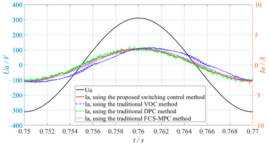
Figure 5.
The A-phase voltage and current simulation waveforms of three-phase VSCs using the proposed method, the VOC method in [7], the DPC method in [8] and the FCS-MPC method in [18] under circuit parameters of L and R uncertainty.
Table 4.
Detailed comparison of different inner loop control methods.
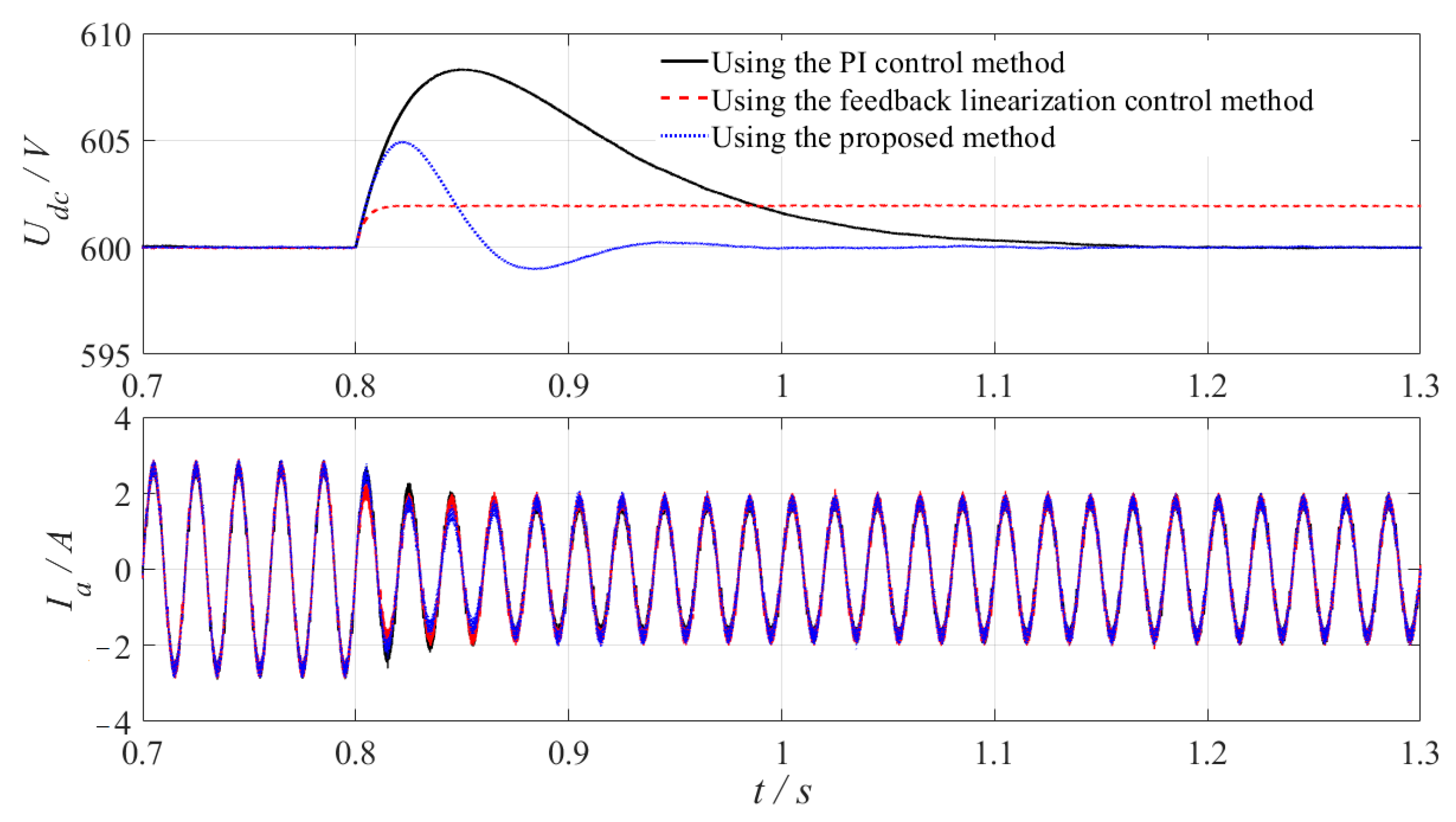
For the robustness of outer loop controller, the load variations are considered, where the load RL suddenly changes from 300 Ω to 450 Ω at 0.8 s. Figure 6 illustrates the simulation comparison results among the traditional PI control method in [7], the traditional feedback linearization method in [32], and the proposed feedback linearization method with SMO under this load variation condition. In Figure 6, the upper panel shows the DC voltage waveforms and the bottom panel shows the A-phase current waveforms. The results in Figure 6 indicate that the traditional PI controller [7] experiences significant fluctuations in DC voltage (9.1 V) and a slow recovery speed (0.38 s) under load variation. In Figure 6, using the traditional feedback linearization method in [8], a steady-state voltage error between the DC voltage and its reference occurs due to discrepancies between the estimated value and actual load in the controller. However, by incorporating SMO, our proposed voltage loop feedback linearization control method achieves smaller fluctuations in DC voltage (5 V) and faster recovery speed (0.22 s). Therefore, it is evident that our proposed voltage loop control method outperforms others.
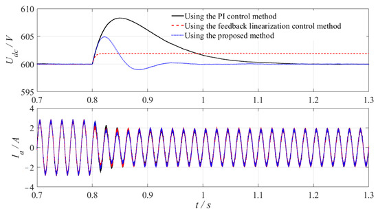
Figure 6.
DC voltage and A-phase current transient state simulation waveforms using the PI control method in [7], the feedback linearization control method in [32] and the proposed method under load variation.
4.2. Experimental Results
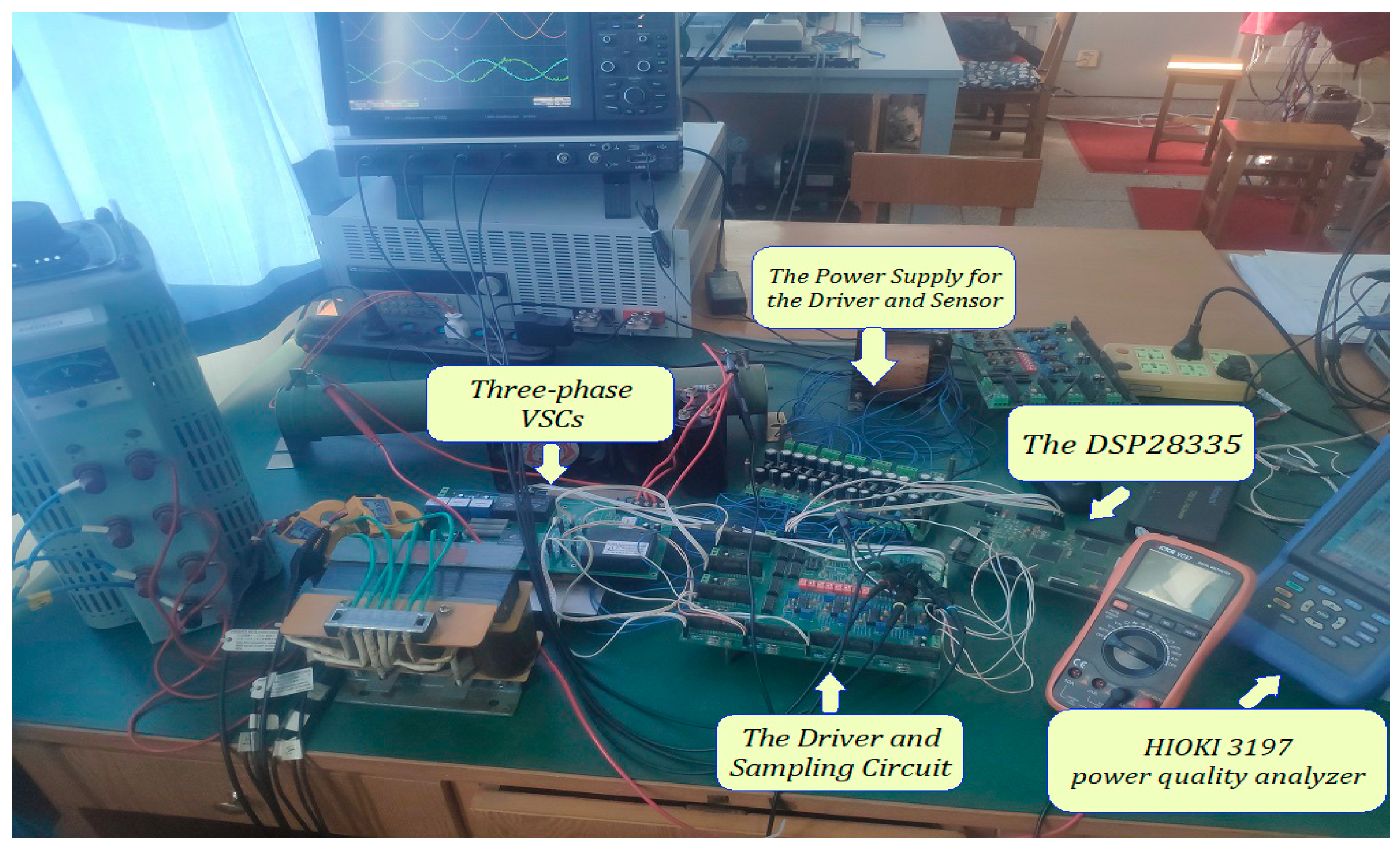
A 1.2 kW three-phase VSC prototype is utilized to validate the efficacy of the control strategies, as shown in Figure 7. The digital controller TMS320F28335 is programmed with control algorithms in the experimental setup, while power quality measurements are conducted using HIOKI 3197 power quality analyzer.

Figure 7.
A photograph of the experimental setup.
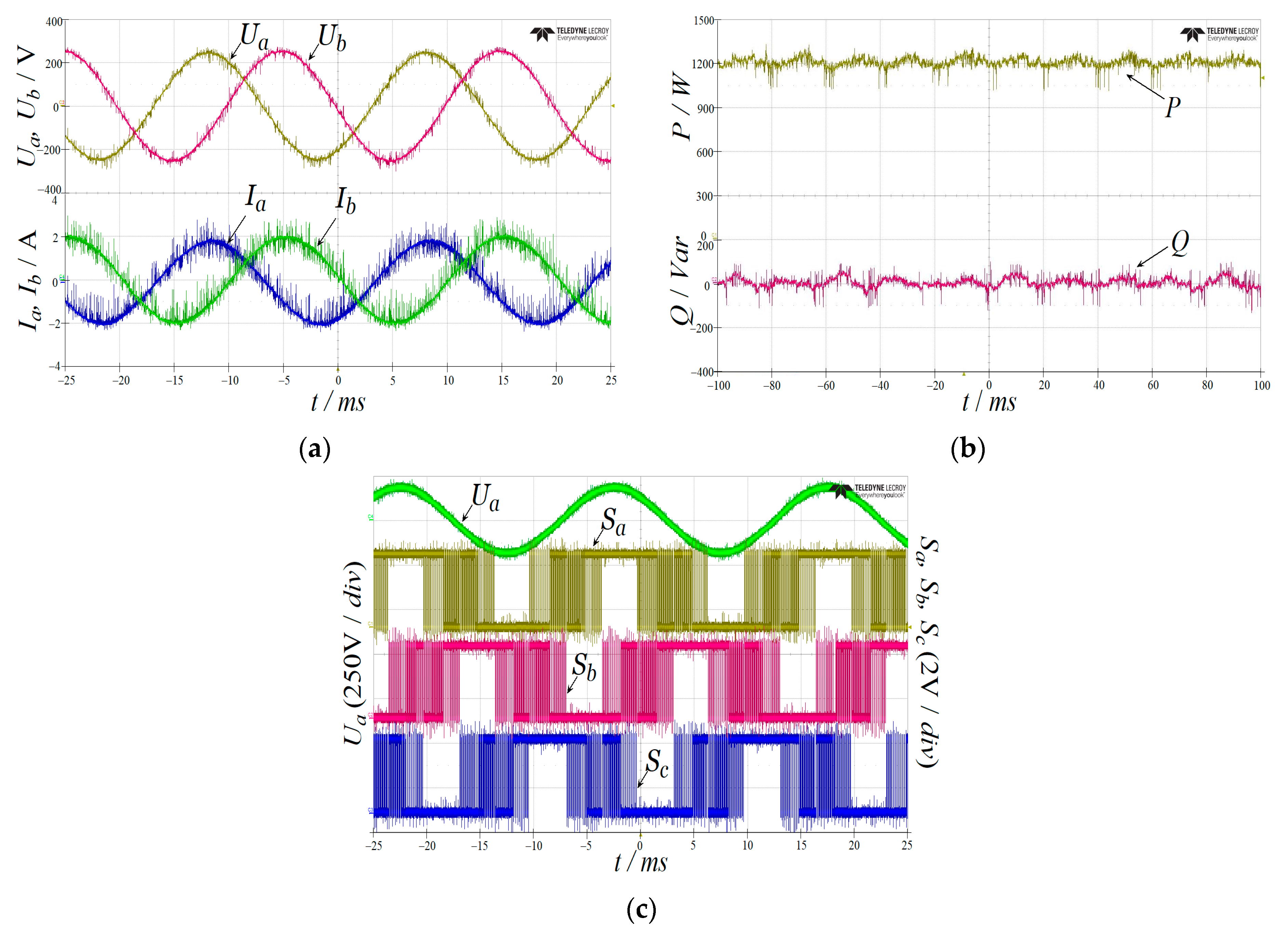
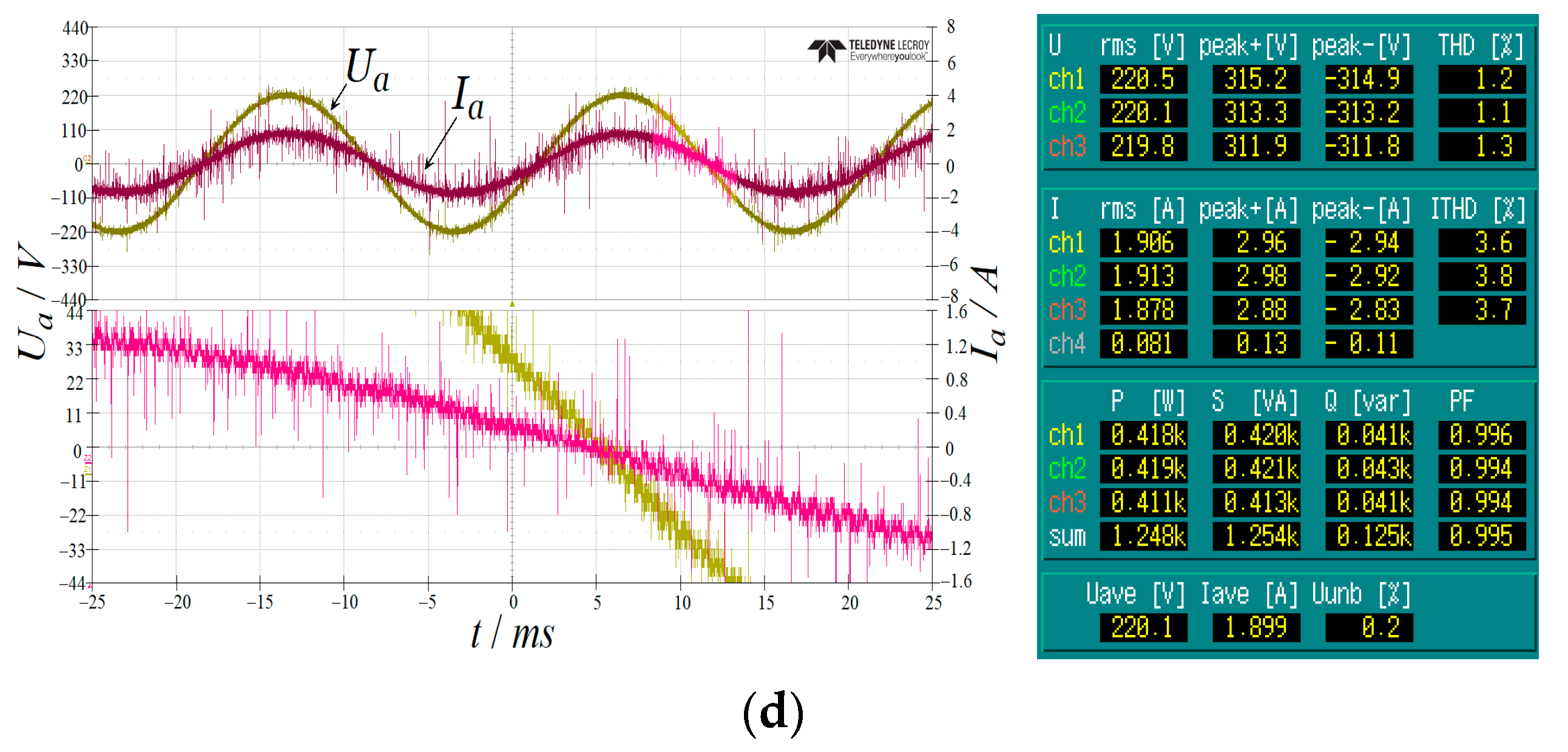
For the practical experimental setup, accurate measurement of actual circuit parameters of three-phase VSCs, such as inductance L, circuit equivalent resistance R, and load RL, is challenging due to their inherent uncertainty and potential variation. In light of this uncertainty in the actual circuit parameters, Figure 8 presents the experimental results of the proposed method for three-phase VSCs. Figure 8a depicts the A- and B-phases voltage and current waveforms, while Figure 8b presents the measured active and reactive power waveforms obtained from D/A channels. Additionally, Figure 8c shows the AC voltage waveform for the A-phase along with the switching states of the three-phase bridge legs. In Figure 8a,b, the proposed method enables the instantaneous regulation of active and reactive power, facilitating the synchronization of three-phase AC voltage and a corresponding current. In Figure 8c, it can be observed that the system achieves direct switching control, wherein one of the three-phase bridge legs maintains a constant switching state within each sector. The experimental results shown in Figure 8 align with the simulation results depicted in Figure 4.

Figure 8.
The experimental results using the proposed method for practical parameters uncertainty: (a) the two-phase voltage and corresponding current waveforms; (b) the active and reactive power waveforms; (c) the A-phase voltage and three-phase switching states waveforms.
Meanwhile, the unity PF and low THD control for three-phase VSCs is achieved using the proposed method, where the average PF is 0.995 and the average THD is 4.7%, as shown in Figure 8c.
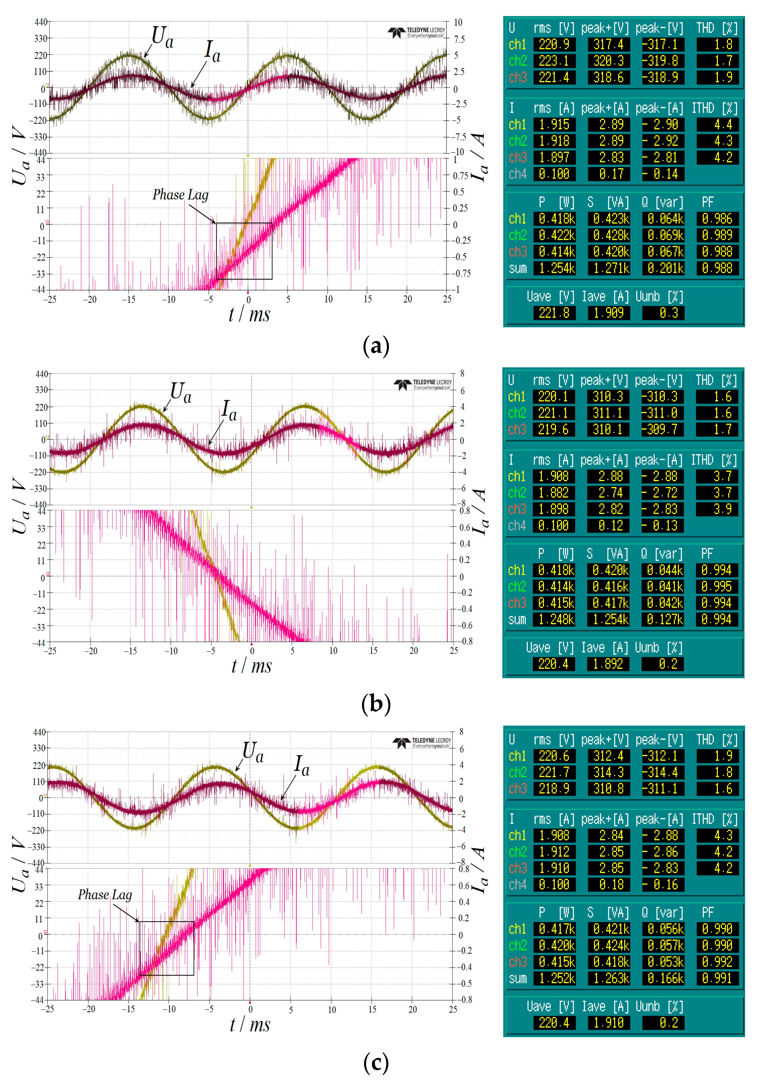
Figure 9a–d display the experimental comparison results of A-phase voltage and current waveforms, as well as the results obtained from HIOKI 3197 power quality analyzer. These comparisons are made between the traditional VOC method in [7], the traditional DPC method in [8], the traditional FCS-MPC method in [18], and the proposed switching control method. It is important to note that these comparisons were conducted while using the nominal values listed in Table 3 for the inner loop controller design of three-phase VSCs. In all subplots on the left side of Figure 9, the upper panel displays the A-phase voltage and current waveforms, while the bottom panel presents enlarged waveforms near the zero-crossing point. The yellow lines represent the voltage curves of phase A, and the red lines represent the current curves of phase A in both panels in Figure 9. In Figure 9a, by using the traditional VOC method in [7], the A-phase current is synchronous to the AC voltage of converter. However, due to the utilization of a decoupled control structure in VOC in [7] and the design of a PI controller based on nominal circuit parameters, the performance of the traditional VOC method described in [7] inevitably deteriorates. There is a phase lag between the A-phase voltage and its corresponding current waveforms in Figure 9a using VOC in [7], resulting in a PF of 0.988 and THD of 4.3%. The traditional DPC method in [8] realizes the active and reactive power control of three-phase VSCs, respectively. It has strong robustness for the circuit parameters uncertainty in Figure 8b, where the PF is 0.994 and THD is 3.76%. However, the parameter tuning of the hysteresis comparators in the traditional DPC method in [8] is difficult. The FCS-MPC method in [18] faces control performance issues under circuit parameter uncertainty due to the inaccuracy parameters used in the predictive model. There is a small phase lag between the A-phase voltage and the corresponding current waveforms in Figure 9c using the MPC method in [18], where PF is 0.991 and THD is 4.23%. Meanwhile, the MPC method in [18] still faces the control parameters tuning difficulty of weights in cost function. The switching rule calculation of the proposed method is unaffected by circuit parameters, in contrast to traditional control methods mentioned above. As a result, Figure 9d demonstrates improved control performance using the proposed method, with a higher PF (0.995) and lower THD (3.7%). The experimental results in Figure 8 align with the simulation results depicted in Figure 5.
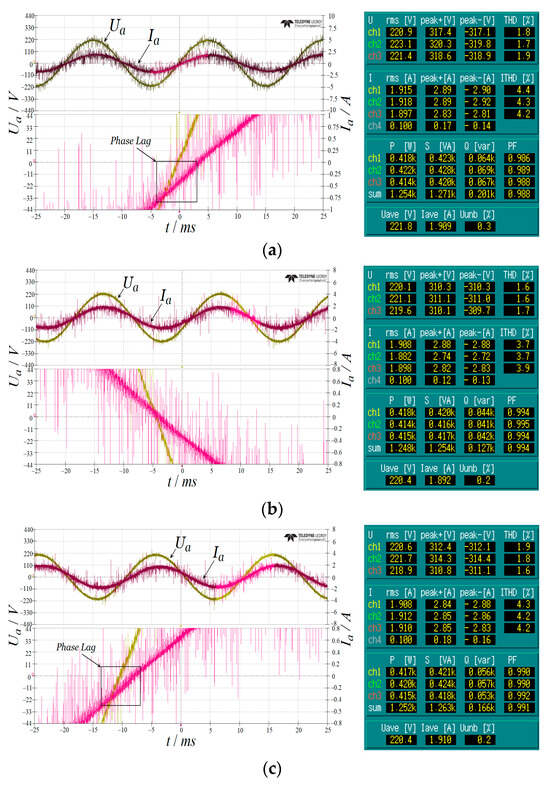
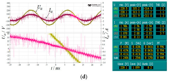
Figure 9.
A-phase voltage and current experiment results of different inner loop control strategies: (a) using the traditional VOC method in [7]; (b) using the traditional DPC method in [8]; (c) using the traditional FCS-MPC method in [18]; (d) using the proposed switching control method.
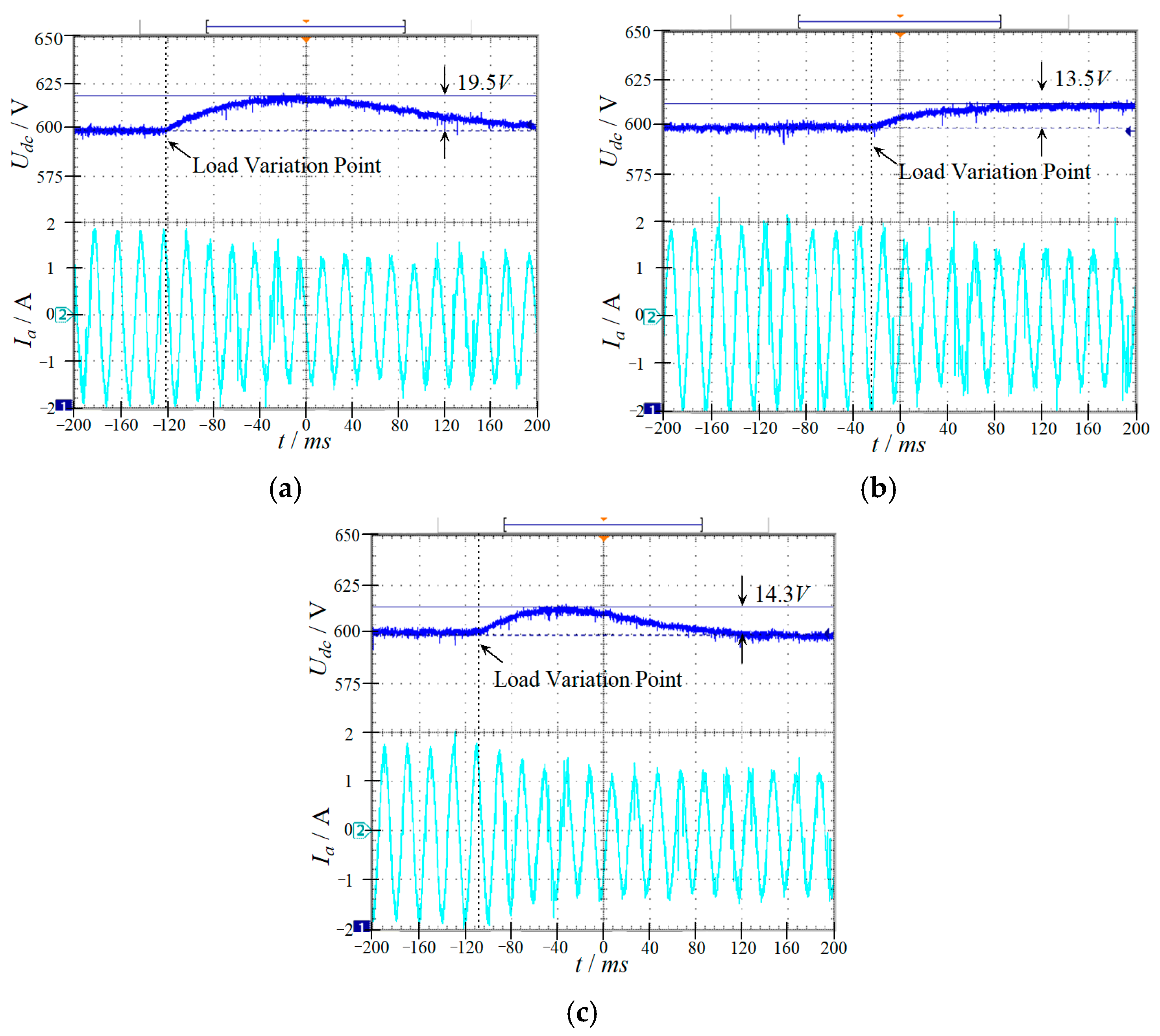
The experimental comparison results of the transient load variation (300 Ω to 450 Ω) among different outer loop control methods are presented in Figure 10, where the proposed power switching control method is employed for the inner controller. In all subplots of Figure 10, the upper panel in all subplots displays the DC voltage waveforms represented by the blue line, while the lower panel illustrates the A-phase current waveforms indicated by the cyan line. From Figure 10, it can be observed that the traditional PI control method described in [7] fails to achieve optimal performance during transient load variation, as evidenced by high voltage perturbation (19.5 V) and slow recovery time (0.32 s), as shown in Figure 10a. Similarly, the traditional feedback linearization control discussed in [32] exhibits a steady-state error (13.5 V) in DC voltage under load variation depicted in Figure 10b. In comparison with these methods, our proposed outer loop controller demonstrates smaller voltage fluctuation (14.3 V) and faster recovery speed (0.23 s), as illustrated in Figure 10c, thereby indicating its superior performance.
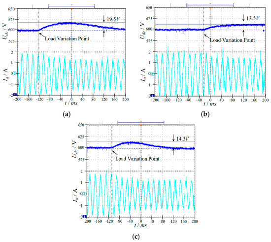
Figure 10.
Experiment comparison results between the different outer voltage loop control methods under transient load variations: (a) using the traditional PI control in [7]; (b) using the traditional feedback linearization control in [32]; (c) using the proposed feedback linearization control with SMO.
5. Conclusions
The paper presents a 2D power switching affine model for three-phase VSCs. Meanwhile, a combined inner loop switching controller and outer loop feedback linearization controller with SMO are proposed to address circuit parameter uncertainty and load variations. Compared to traditional linearized modeling and control methods, the proposed approach achieves superior performance with simpler control structure and fewer control parameters, resulting in improved static and transient performance related to PF and voltage fluctuation. Despite the challenge of the unfixed switching frequency inherent in the proposed method, it still presents considerable improvements over traditional control strategies.
Author Contributions
Conceptualization, methodology, and writing—original draft preparation, X.G.; software and validation, J.Q.; formal analysis, Y.L.; writing—review and editing, supervision, and project administration, S.J. All authors have read and agreed to the published version of the manuscript.
Funding
This research was funded partly by National Natural Science Foundation of China, grant number 62371388, 61803300, 62103327.
Data Availability Statement
Data are contained within the article.
Conflicts of Interest
We declare that we have no financial and personal relationships with other people or organizations that can inappropriately influence our work; there is no professional or other personal interest of any nature or kind in any product, service, and/or company that could be construed as influencing the position presented in, or the review of, the manuscript entitled “A Robust Switching Control Strategy for Three-Phase Voltage Source Converters with Uncertain Circuit Parameters ”.
References
- Chandwani, A.; Mallik, A. A reduced stage configuration of three-phase isolated AC/DC converter for auxiliary power units. IEEE Trans. Veh. Technol. 2022, 71, 3687–3703. [Google Scholar] [CrossRef]
- Ma, K.; Wang, J.S.; Cai, X.; Blaabjerg, F. AC grid emulations for advanced testing of grid-connected converters—An overview. IEEE Trans. Power Electr. 2021, 36, 1626–1645. [Google Scholar] [CrossRef]
- Chen, H.; Xu, D.G.; Deng, X. Control for power converter of small-scale switched reluctance wind power generator. IEEE Trans. Ind. Electron. 2021, 68, 3148–3158. [Google Scholar] [CrossRef]
- Wang, P.; Chen, X.Z.; Tong, C.N.; Jia, P.Y.; Wen, C.X. Large- and small-signal average-value modeling of dual active-bridge DC-DC converter with triple-phase-shift control. IEEE Trans. Power Electron. 2021, 36, 9237–9250. [Google Scholar] [CrossRef]
- Yue, X.L.; Wang, X.F.; Blaabjerg, F. Review of small-signal modeling methods including frequency-coupling dynamics of power converters. IEEE Trans. Power Electron. 2019, 34, 3313–3328. [Google Scholar] [CrossRef]
- Liao, Y.C.; Wang, X.F. Small-signal modeling of AC power electronic systems: Critical review and unified modeling. IEEE Open J. Power Electron. 2021, 2, 424–439. [Google Scholar] [CrossRef]
- Guo, X.; Ren, H.P.; Liu, D. An optimized PI controller design for three- phase PFC converter based on multi-objective chaotic particle swarm optimization. J. Power Electron. 2016, 16, 610–620. [Google Scholar] [CrossRef]
- Gui, Y.H.; Kim, C.H.; Chung, C.C.; Guerrero, J.M.; Guan, Y.J.; Vasquez, J.C. Improved direct power control for grid-connected voltage source converters. IEEE Trans. Ind. Electron. 2018, 65, 8041–8051. [Google Scholar] [CrossRef]
- Jeeranantasin, N.; Nungam, S. Sliding mode control of three-phase AC/DC converters using exponential rate reaching law. J. Syst. Eng. Electron. 2022, 33, 210–221. [Google Scholar] [CrossRef]
- Ren, H.P.; Guo, X. Robust adaptive control of a CACZVS three-phase PFC converter for power supply of silicon growth furnace. IEEE Trans. Ind. Electron. 2016, 63, 903–912. [Google Scholar] [CrossRef]
- Hasanien, H.M.; Matar, M. A fuzzy logic controller for autonomous operation of a voltage source converter-based distributed generation system. IEEE Trans. Smart Grid 2015, 6, 158–165. [Google Scholar] [CrossRef]
- Hou, L.M.; Ma, J.H.; Wang, W. Sliding mode predictive current control of permanent magnet synchronous motor with cascaded variable rate sliding mode speed controller. IEEE Access 2022, 10, 33992–34002. [Google Scholar] [CrossRef]
- Yin, Y.F.; Liu, J.X.; Luo, W.S.; Wu, L.G.; Vazquez, S.; Leon, J.I.; Franquelo, L.G. Adaptive control for three-phase power converters with disturbance rejection performance. IEEE Trans. Syst. Man Cybern. Syst. 2021, 51, 674–685. [Google Scholar] [CrossRef]
- Dyhia, K.; Hakim, D.; Lamine, H.M.; Arezki, F.; Nacereddine, B. Comparative study of PI and fuzzy logic controllers for three-phases parallel multi-cell converter. In Proceedings of the International Conference on Control, Automation and Diagnosis, Grenoble, France, 2–4 July 2019. [Google Scholar]
- Shieh, C.S. Quick implementation of pule wise modulation (PWM), pulse frequency modulation (PFM) and mixed PWM/PFM on FPGA chip. In Proceedings of the International Symposium on Computer, Consumer and Control, Taichung City, Taiwan, 13–16 November 2020. [Google Scholar]
- Holmes, D.G.; Lipo, T.A. Pulse Width Modulation for Power Converters: Principles and Practice; Wiley-IEEE Press: Hoboken, NJ, USA, 2003. [Google Scholar]
- Khalilzadeh, M.; Vaez-Zadeh, S.; Rodriguez, J.; Heydari, R. Model-free predictive control of motor drives and power converters: A review. IEEE Access 2020, 9, 105733–105747. [Google Scholar] [CrossRef]
- Zhao, Z.L.; Gong, S.Q.; Yang, Q.G.; Xie, J.D.; Luo, X.; Zhang, J.X.; Ni, Q.; Lai, L.L. An improved FCS-MPC strategy for low-frequency oscillation stabilization of PV-based microgrids. IEEE Trans. Sustain. Energy 2023, 14, 2376–2390. [Google Scholar] [CrossRef]
- Li, X.Y.; Tian, W.; Gao, X.N.; Yang, Q.F.; Kennel, R. A generalized observer-based robust predictive current control strategy for PMSM drive system. IEEE Trans. Ind. Electron. 2022, 69, 1322–1332. [Google Scholar] [CrossRef]
- Guo, X.; Ren, H.P.; Li, J. Robust model predictive control for compound active clamp three-phase soft switching PFC converter under unbalanced grid condition. IEEE Trans. Ind. Electron. 2018, 65, 2156–2166. [Google Scholar] [CrossRef]
- Vazquez, S.; Rodriguez, J.; Rivera, M.; Franquelo, L.G.; Norambuena, M. Model predictive control for power converters and drives: Advances and trends. IEEE Trans. Ind. Electron. 2017, 64, 935–947. [Google Scholar] [CrossRef]
- Li, C.W.; Tang, H.H.; Zheng, X.S.; Rong, H.J. Modeling and quadratic optimal control of three-phase APF based on switched system. Proc. CSEE 2008, 28, 66–72. [Google Scholar]
- Ding, Q.Q.; Tang, H.H.; Rong, Y.J.; Jiao, F. Modeling and h∞ control of three-phase APF based on switched system. Trans. China Electrotech. Soc. 2008, 23, 125–131. [Google Scholar]
- Egidio, L.N.; Deaecto, G.S.; Barros, T.A. Switched control of a three-phase AC-DC power converter. IFAC-PapersOnLine 2020, 53, 6471–6476. [Google Scholar] [CrossRef]
- Li, X.F.; Qu, L.L.; Ren, W.D.; Zhang, C.X.; Liu, S.Y. Controllability of the three-phase inverters based on switched linear system model. In Proceedings of the IEEE International Conference on Industrial Technology, Taipei, Taiwan, 14–17 March 2016. [Google Scholar]
- Tian, C.Y.; Li, K.; Zhang, C.H.; Zhuang, F.F.; Ye, B.S. Control strategy for bi- directional AC-DC converter based on switched system model. Trans. China Electrotech. Soc. 2015, 30, 70–76. [Google Scholar]
- Guo, X.; Ren, H.P. A switching control strategy based on switching system model of three-phase VSR under unbalanced grid conditions. IEEE Trans. Ind. Electron. 2021, 68, 5799–5809. [Google Scholar] [CrossRef]
- Bolzern, P.; Spinelli, W. Quadratic stabilization of a switched affine system about a nonequilibrium point. In Proceedings of the 2004 American Control Conference, Boston, MA, USA, 30 June–2 July 2004. [Google Scholar]
- Della Rossa, M.; Egidio, L.N.; Jungers, R.M. Stability of switched affine systems: Arbitrary and dwell-time switching. arXiv 2022, arXiv:2203.06968. [Google Scholar] [CrossRef]
- Yan, S.; Yang, Y.H.; Hui, S.Y.; Blaabjerg, F. A review on direct power control of pulse width modulation converters. IEEE Trans. Power Electron. 2021, 36, 11984–12007. [Google Scholar] [CrossRef]
- Guo, X.; Ren, H.P. Nonlinear feedback control of compound active-clamp soft-switching three-phase PFC converter base on load observer. In Proceedings of the IEEE Energy Conversion Congress and Exposition, Pittsburgh, PA, USA, 14–18 September 2014. [Google Scholar]
- Bao, X.W.; Zhuo, F.; Tian, Y.; Tan, P.X. Simplified feedback linearization control of three-phase photovoltaic inverter with an LCL filter. IEEE Trans. Power Electron. 2013, 28, 2739–2752. [Google Scholar] [CrossRef]
- Golestan, S.; Guerrero, J.M.; Vasquez, J.C. Three-phase PLLs: A review of recent advances. IEEE Trans. Power Electron. 2017, 32, 1894–1907. [Google Scholar] [CrossRef]

Disclaimer/Publisher’s Note: The statements, opinions and data contained in all publications are solely those of the individual author(s) and contributor(s) and not of MDPI and/or the editor(s). MDPI and/or the editor(s) disclaim responsibility for any injury to people or property resulting from any ideas, methods, instructions or products referred to in the content. |
© 2024 by the authors. Licensee MDPI, Basel, Switzerland. This article is an open access article distributed under the terms and conditions of the Creative Commons Attribution (CC BY) license (https://creativecommons.org/licenses/by/4.0/).