Research on Off-Design Characteristics and Control of an Innovative S-CO₂ Power Cycle Driven by the Flue Gas Waste Heat

Abstract

Recently, supercritical CO₂ (S-CO₂) has been extensively applied for the recovery of waste heat from flue gas. Although various cycle configurations have been proposed, existing studies predominantly focus on the steady analysis and optimization of different S-CO₂ structures under design conditions, and there is a noticeable deficiency in off-design research, especially for the innovative S-CO₂ cycles. Thus, in this work aimed at the proposed novel S-CO₂ power cycle, off-design characteristics and corresponding control strategies are investigated for the waste heat recovery. Based on the design parameters of the S-CO₂ cycle, structural dimensions of printed circuit heat exchangers (PCHEs) and shell-and-tube heat exchangers are determined, and design values of turbines and compressors are specified. On this basis, off-design models for these key components are formulated. By manipulating variables such as cooling water inlet temperature, cooling water mass flow rate, flue gas inlet temperature and flue gas mass flow rate, cycle performances of the system are analyzed under off-design conditions. The simulation results show that when the inlet temperature and the mass flow rate of cooling water vary separately, the thermal efficiency both can reach the maximum value of 28.43% at the design point. For the changes in heat source parameters, the optimum point is slightly deviated from the design condition. Amidst the fluctuations in flue gas inlet temperature, the thermal efficiency optimizes to a peak of 28.56% at 530 °C. In the case of variation in the flue gas mass flow rate, the highest thermal efficiency 28.75% can be obtained. Furthermore, to maintain the efficient and stable operation of the S-CO₂ power cycle, the corresponding control strategy of the cooling water mass flow rate is proposed for the cooling water inlet temperature variation. Generally, when the inlet temperature of cooling water increases from 23 °C to 27 °C, the cooling water mass flow should increase from 82.3% to 132.7% of the design value to keep the system running as much as possible at design conditions.

1. Introduction

1.1. Background

Currently, fossil fuel energy is still the main source of energy with the increase in primary energy consumption. However, the burning of coal, oil and other fossil fuels generates a high amount of environmentally unfriendly gases, among which carbon dioxide causes a serious greenhouse effect [1,2]. To alleviate the dilemma of energy scarcity while reducing the environmental impact of fossil fuels, it is imperative to enhance energy efficiency. The waste heat from industrial waste gas has great recovery potential, and scholars have extensively conducted research on the comprehensive recovery and optimal utilization of industrial waste heat without interfering with the original industrial manufacturing process [3,4]. The organic Rankine cycle (ORC) holds a pivotal position in the realm of low temperature thermal power generation due to the low critical parameters of the organic working fluid [5,6]. Although ORC is a mature technology that offers the advantages of low maintenance costs, high operating pressure and autonomous operation, it still suffers from disadvantages such as a low boiling point of organic working fluid, low waste heat recovery efficiency, environmental pollution and safety issues [7,8]. In the case of high-temperature waste heat utilization, the technically mature steam Rankine cycle is usually used. However, the steam Rankine cycle has high heat loss, a large component volume and high system cost [9]. In recent years, in view of the shortcomings of the existing steam Rankine cycle and the low critical parameters of CO₂ (Tc = 30.98 °C, Pc = 7.38 MPa), scholars have proposed the application of the supercritical CO₂ (S-CO₂) Brayton power cycle to recover the waste heat of high temperature flue gas [10,11]. In contrast with the steam Rankine cycle, the S-CO₂ cycle has the advantages of a compact system structure, a low cost and high cycle efficiency [12].

1.2. Study on S-CO₂ Cycle Layout and Performance

In order to improve thermal efficiency, scholars in various countries have conducted many studies on optimizing the S-CO₂ cycle. One approach is to combine thermodynamic processes such as multi-stage compression, segmented expansion and reheating on the basis of a simple S-CO₂ cycle [13,14]. Several typical layouts of S-CO₂ cycles have been formed, including the simple recuperative cycle (SRC), the recompression cycle (RC), the precompression cycle (PC), the partial cooling cycle (PCC), the intermediate cooling cycle (ICC), and their layouts with reheating. Liao et al. analyzed five types of cycles and compared the cycle efficiencies of the five cycle systems under the same operating parameters, which showed that both the recompression cycle and the partial cooling cycle exhibit superior efficiency, while no significant advantage in efficiency is observed for the partial cooling cycle under low pressure ratios [15]. Fang et al. introduced a waste heat recovery system predicated on the split expansion cycle. Compared to the conventional recompression cycle, the fuel utilization rate of a 1 MW natural gas engine increases by 14.9%, while achieving the net power and heat recovery rates of 174.2 kW and 58%, respectively [16]. Another enhancement approach involves designing a combined cycle layout with the S-CO₂ cycle serving as the top cycle [13]. Given that the primary function of the bottom cycle is to capture low-grade waste heat from the top cycle, the transcritical CO₂ cycle (T-CO₂), ORC, and refrigeration cycle are all integrated with the S-CO₂ cycle, forming well-combined cycles. Fu used the S-CO₂ Brayton cycle as the top cycle and combined it with an ORC system or a T-CO₂ cycle system to establish a combined cycle with different layouts. The performance of the combined cycle exhibited notable enhancements compared to the stand-alone S-CO₂ Brayton cycle. Moreover, in the recompression S-CO₂/ORC combined cycle, system efficiency reached its peak when employing isopentane as the working fluid in the ORC [17]. The above research results show that the improvement of thermal efficiency is closely related to the S-CO₂ cycle structure, and the different configuration of the cycle system has a crucial impact on the performance of the cycle.

1.3. Study on Off-Design Performance of S-CO₂ Cycle

The above studies, all analyzed with the key system parameters unchanged, evaluated the steady-state performance of different S-CO₂ systems. In practical applications, the performances of systems are likely to vary due to the fluctuations in cold and heat source conditions influenced by environmental changes. To advance the practical engineering application of the S-CO₂ power cycle, it is imperative to analyze and study the performance characteristics of the cycle under off-design conditions, so as to solve the problems that may occur in the actual operation of the system. Andrew et al. studied the off-design operation of the S-CO₂ cycle by utilizing head and efficiency curves proposed by Dyreby. They modified the dimensionless compression ratio and isentropic efficiency of the compressor based on these curves to characterize the performance characteristics of the compressor under off-design operating conditions [18]. Duniam et al. conducted a study examining the influence of ambient temperature at design values on the operational performance of the S-CO₂ recompression Brayton cycle under off-design conditions. The results showed that the lower the design value, the higher the peak efficiency. However, the declines in efficiency are greater with the increase in ambient temperature, and the benefit of low ambient temperature is limited when the design values are higher [19]. In conclusion, these existing studies focus more on the off-design performance analysis of typical S-CO₂ cycles and system components, and there is still a lack of studies on off-design conditions for novel S-CO₂ cycles.

1.4. Purpose of This Work

The system can run efficiently and stably by adjusting the key parameters when the external conditions change, so it is necessary to study the off-design characteristics of the cycle. Based on an innovative S-CO₂ power cycle driven by flue gas waste heat proposed by our research group [20], off-design characteristics and corresponding control strategies are studied in this paper. Based on the design parameters of the S-CO₂ cycle, along with the determined structural parameters of heat exchangers and performance parameters of the turbomachinery, off-design mathematical models are developed for the system components. Subsequently, according to the simulation results, the performance characteristics of the system are analyzed when the parameters of cold and hot sources change. In addition, since the cooling water inlet temperature is prone to affect the cycle performance, a cooling water mass flow rate control strategy is proposed to ensure the stable and efficient operation of the cycle.

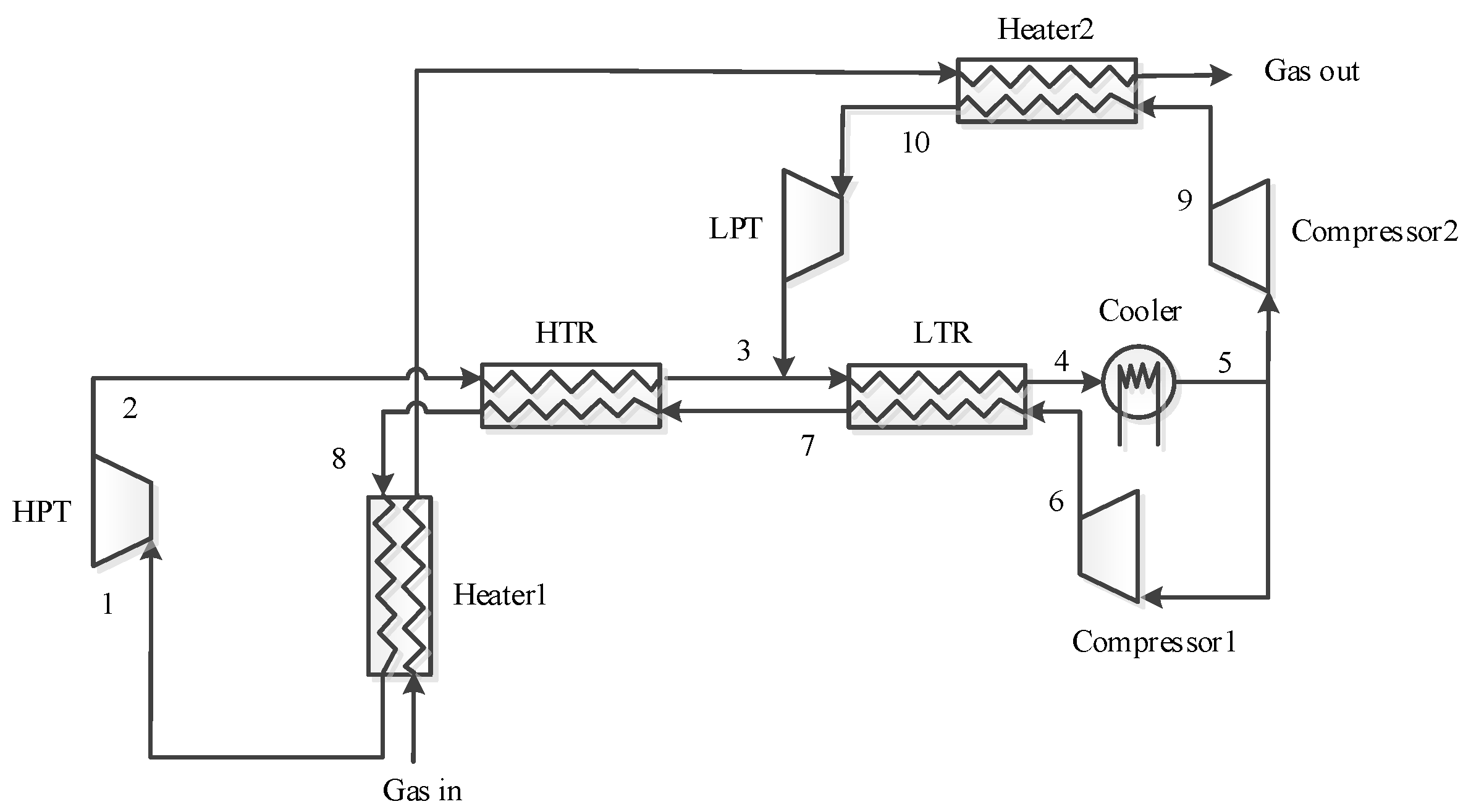
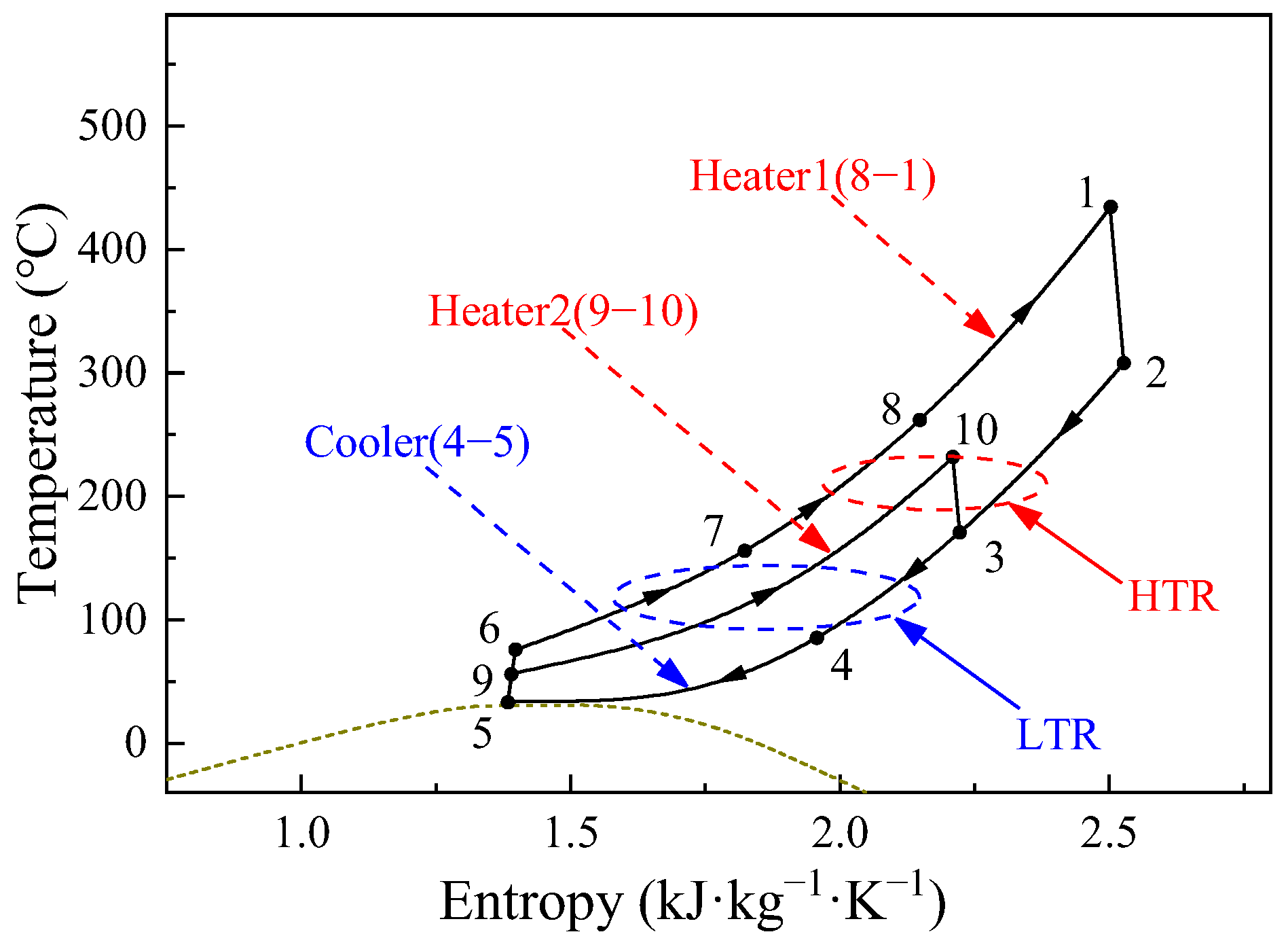
2. System Layout and Design Parameters

Figure 1 illustrates the layout of the S-CO₂ power cycle driven by flue gas waste heat, and the corresponding T-s diagram is shown in Figure 2. S-CO₂ is divided into two streams at the outlet of the cooler. One stream is compressed in Compressor1 (5–6), and then successively flows into the high-pressure side of the low-temperature recuperator (LTR, 6–7) and the high-temperature recuperator (HTR, 7–8) to be heated. After that, S-CO₂ further absorbs waste heat from the flue gas in Heater1, expanded to carry out work in the high-pressure turbine (HPT, 1–2), and finally cooled by HTR (2–3), LTR (3–4), and the cooler (4–5). Another stream of S-CO₂ is first compressed in Compressor2 (5–9), and then heated by the flue gas in Heater2 (9–10). After being heated, S-CO₂ is expanded into the low-pressure turbine (LPT, 10–3) to carry out work, and finally S-CO₂ is mixed with another stream of fluid at the low-pressure outlet of HTR.

The composition and parameters of the flue gas are obtained from a diesel engine, as shown in

Table 1. Main parameters of flue gas [20,21].

Flue Gas Components	Value	Flue Gas Parameters	Value
N2 (%)	71.6	Flue gas inlet temperature (°C)	520
CO2 (%)	15.1	Flue gas mass flow (kg/s)	20
O2 (%)	7.8	Flue gas pressure (MPa)	0.1
H2O (%)	5.5

. Besides the components listed in Table 1, the flue gas mixture also contains SO₂, SO₃, NO_X and other components. However, they are not included in the table because of the extremely low content and small impact on the heat transfer characteristics of the flue gas.

For the cycle, the parameters of design conditions are shown in

Table 2. System standard design conditions.

Design Parameters	Value
HPT inlet temperature (°C)	434.35
Compressor inlet temperature (°C)	33
HPT inlet pressure (MPa)	25
LPT inlet pressure (MPa)	15
Compressor inlet pressure (MPa)	7.8
PPTD of Heater1 (°C)	20
PPTD of Heater2 (°C)	20
PPTD of HTR (°C)	≥5
PPTD of LTR (°C)	≥5
Isentropic efficiency of Compressor [20]	0.85
Isentropic efficiency of Turbine [20]	0.9
Energy efficiency coefficient of heat exchanger [20]	0.9

. The high pressure, medium pressure and low pressure of the cycle are set to be 25 MPa, 15 MPa and 7.8 MPa, respectively. The compressor inlet temperature represents the minimum cycle temperature, which is set at 33 °C. For the pinch point temperature difference (PPTD), considering the heat exchange efficiency and heat exchanger economy, the PPTD of the heat exchangers are set above 5 °C. Under the design conditions, the parameters of each state point of the cycle are shown in

Table 3. Parameters of each state point of the cycle.

State Point	m (kg/s)	P (MPa)	T (°C)	s (kJ/(kg·K))	h (kJ/kg)
1	24.44	25	434.35	2.5	887.36
2	24.44	7.8	307.9	2.53	762.17
3	37.94	7.8	170.52	2.22	606.76
4	37.94	7.8	85.16	1.96	501.11
5	37.94	7.8	33	1.38	318.06
6	24.44	25	75.32	1.4	349.02
7	24.44	25	155.6	1.82	513.01
8	24.44	25	261.73	2.15	668.43
9	13.5	15	55.66	1.39	331.95
10	13.5	15	231.66	2.21	654.43
Flue gas inlet	20	0.1	520	7.2	959.9
Flue gas outlet of Heater1	20	0.1	281.73	6.8	692.32
Flue gas outlet	20	0.1	75.69	6.31	474.63
cooling water inlet	110.79	0.1	25	0.37	104.92
cooling water outlet	110.79	0.1	40	0.57	167.62

.

For the performances of the S-CO₂ Brayton cycle, the evaluation indexes include the thermal efficiency (η_th) and net output work (W_net) of the cycle. In order to obtain these data, the expansion work, compression work and total heat absorption of the cycle should be calculated.

The W_net is the difference between the work of expansion and the work of compression, which can be expressed by

$$W_{\mathrm{net}}=W_{\mathrm{HPT}}+W_{\mathrm{LPT}}-W_{\mathrm{Compressor}1}-W_{\mathrm{Compressor}2}$$

(1)

The η_th is the ratio of W_net to the total heat absorbed by the flue gas heat source, which is calculated as follows:

$${\eta }_{\mathrm{th}}=\frac{W_{\mathrm{net}}}{Q_{\mathrm{Heater}1}+Q_{\mathrm{Heater}2}}$$

(2)

3. Structural Design and Off-Design Models of Heat Exchangers

The heat exchangers in the system include a cooler, two heaters and two recuperators. The fluids used in the heat exchangers include CO₂, flue gas and water. To simplify heat transfer calculations, thermodynamic modeling makes the following assumptions:

• The pressure drop of the heat exchangers caused by inlet losses, outlet losses and acceleration effects is neglected.
• The fluids are fully mixed in the tube and flow one-dimensionally.
• The heat conduction between the fluids and the tube wall along the axial direction is ignored.
• The heat transfer with the external environment is ignored.

Based on the above assumptions and the heat transfer condition of the cycle, printed circuit heat exchangers (PCHEs) and shell-and-tube heat exchangers are used to complete the heat transfer in the system.

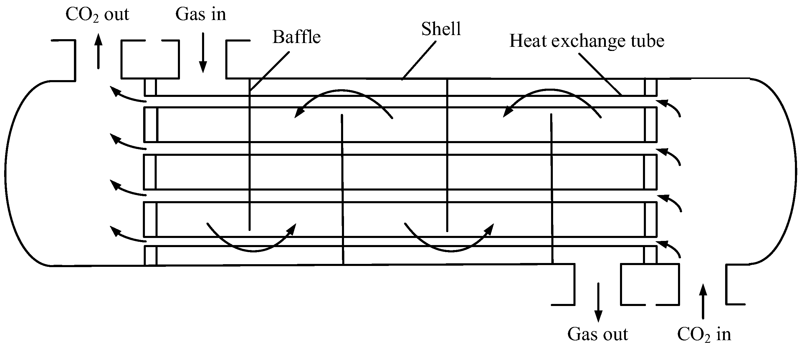
3.1. Structural Design of Heat Exchangers

The off-design performances of the system are affected by the capacity constraints of the system components. Therefore, the heat exchangers should first be designed. The structural design parameters of PCHEs and shell-and-tube heat exchangers are obtained by calculating the parameters of each state point under the design conditions, as shown in

Table 4. Structural design parameters of PCHEs.

Parameters	HTR	LTR	Cooler
Channel width (mm)	1	1	1
Channel depth (mm)	1	1	1
Plate thickness (mm)	1.5	1.5	1.5
Fin width (mm)	0.5	0.5	0.5
Number of channels per layer	300	300	300
Number of plies	300	300	300
Single channel heat transfer area (m2)	0.025	0.05	0.036

and

Table 5. Structural design parameters of shell-and-tube heat exchangers.

Parameters	Heater1	Heater2
Number of one-way tubes	484	237
One way tube length (m)	16.64	40.44
Length of tube (m)	5	7
Number of tube sides	4	6
Number of shell sides	2	2
Number of centerline tubes	48	41
Calculated nominal diameter (m)	1.77	1.51
Nominal diameter (m)	1.8	1.6
Inside diameter of tube (m)	0.02	0.02
Outer diameter of tube (m)	0.025	0.025
Tube wall thickness (m)	0.0025	0.0025
Tube pitch (m)	0.032	0.032
Pipe flow area (m2)	0.0003	0.0003
Baffle thickness (m)	0.012	0.012
Baffle spacing (m)	0.3	0.3
Number of baffles	52	126
Total heat transfer area (m2)	596.97	706.9
Area margin	17.20%	1.65%
CO2 tube velocity (m/s)	0.75	0.75
Flue gas center velocity (m/s)	204.26	142.83
Pipe pressure drop (kPa)	7.93	17.41
Pipe volume (m3)	3.04	3.13
Heat transfer coefficient of CO2 (W/(m2·k))	535.34	575.07
Heat transfer coefficient of flue gas (W/(m2·k))	380.22	324.64

.

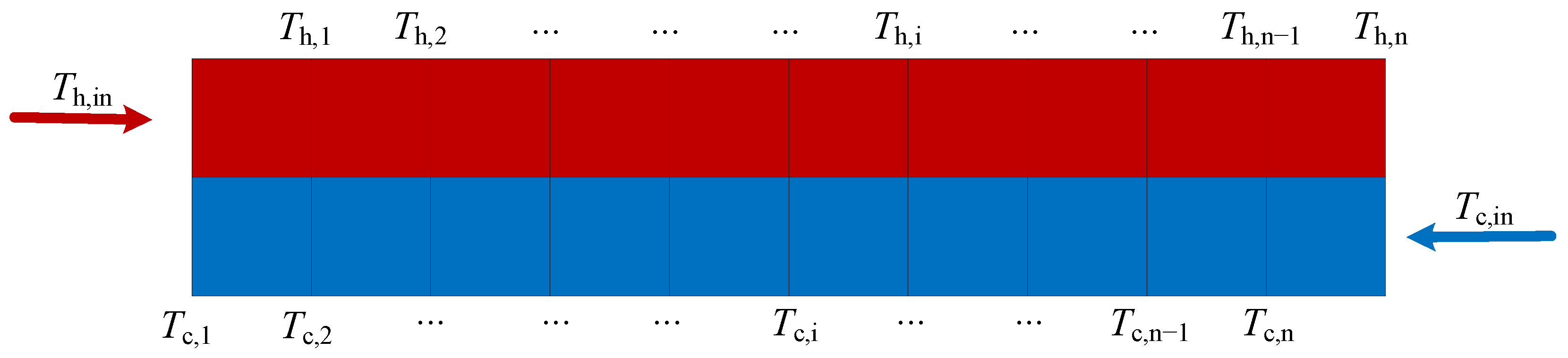
3.2. Off-Design Models of Heat Exchangers

3.2.1. Off-Design Models of PCHEs

Compared with traditional heat exchangers, micro-channel heat exchangers can significantly reduce the volume and greatly enhance the heat transfer efficiency while maintaining the same heat transfer capacity. In this way, they have been widely used in many important fields. Among them, PCHE is widely used in the S-CO₂ energy system due to its advantages of high-temperature and high-pressure resistance, high compactness and high reliability [22]. Therefore, the HTR and LTR of the S-CO₂ cycle adopt counter current S-shaped fin PCHEs. For the cooler, the S-CO₂ fluid is cooled by water cooling. The density of water at normal temperature and pressure is the same order of magnitude as that of S-CO₂, and the treated water has less corrosion on the PCHE micro-channels. Thus, the cooler of the system uses the same PCHE as the recuperators. Taking into account periodic boundary conditions, the PCHE model is simplified to a single channel. It consists of a hot and a cold side channel. Furthermore, the heat transfer parameters of each channel unit in a single layer are considered to be the same [23].

The single channel unit heat transfer rate Q_ch is:

$$Q_{\mathrm{ch}}=\frac{Q}{a}$$

(3)

where Q is the total heat transfer rate, and a is the total number of channel units of cold or hot fluid [24].

As shown in Figure 3, the inlet temperatures of the hot and cold fluids of the PCHE are T_h,in and T_c,in, respectively. A single channel unit is divided into n segments along the flow direction, and each segment is regarded as a separate subunit. The heat transfer rate of each subunit Q_ch,i is formulated as:

$$Q_{\mathrm{ch},\mathrm{i}}=\frac{Q_{\mathrm{ch}}}{n}$$

(4)

Based on the parameters of each heat exchange subunit, the heat exchange area A_ch,i can be calculated as

$$A_{\mathrm{ch},\mathrm{i}}=\frac{Q_{\mathrm{ch},\mathrm{i}}}{k_{\mathrm{i}}\cdot \mathsf{\Delta }{T}_{\mathrm{i}}}$$

(5)

where ΔT_i represents the arithmetic average temperature difference between the cold and hot streams in section i, and k represents the local heat transfer coefficient, which can be expressed by Equation (6).

$$k=\frac{1}{\frac{1}{h_{\mathrm{h}}}+R_{\mathrm{w}}+\frac{1}{h_{\mathrm{c}}}}$$

(6)

where R_w denotes the thermal resistance of the channel wall, h_h and h_c represent the convective heat transfer coefficients of hot and cold fluids, respectively.

The convective heat transfer coefficient h can be expressed in the following way:

$$h=\frac{\lambda \cdot Nu}{d_{\mathrm{hy}}}$$

(7)

where λ denotes the thermal conductivity of the fluid and d_hy denotes the hydraulic diameter of the channel.

The heat transfer correlations used for the PCHE models in the system are shown in

Table 6. Heat transfer correlations of PCHE models.

Category	Heat Transfer Correlations	References
The S-CO2 side of LTR, HTR, and cooler	$Nu=0.174{\mathit{Re}}^{0.593}{\mathit{Pr}}^{0.43}$	[23,25]
The water side of cooler	$Nu=\frac{\frac{f}{8}(\mathit{Re}-1000)\mathit{Pr}}{1+12.7\sqrt{\frac{f}{8}}\left({\mathit{Pr}}^{2/3}-1\right)},2300\le \mathit{Re}\le {10}^6,0.6\le \mathit{Pr}\le {10}^5$ $f={(0.79\times \ln \left(\mathit{Re}\right)-1.64)}^{-2}$	[26]

.

Channel hydraulic diameter d_hy can be represented by Equation (8).

$$d_{\mathrm{hy}}=\frac{2\cdot w_{\mathrm{ch}}\cdot d_{\mathrm{ch}}}{w_{\mathrm{ch}}+d_{\mathrm{ch}}}$$

(8)

where w_ch is the channel width and d_ch is the channel height. Based on these two parameters, the flow area A_flow of the channel can be calculated as

$$A_{\mathrm{flow}}=w_{\mathrm{ch}}\cdot d_{\mathrm{ch}}$$

(9)

Channel wall thermal resistance R_w can be expressed as

$$R_{\mathrm{w}}=\frac{t_{\mathrm{p}}-d_{\mathrm{ch}}}{{\lambda }_{\mathrm{w}}}$$

(10)

where t_p represents the thickness of the heat exchange plate, λ_w represents the thermal conductivity of the wall of the channel.

The total heat transfer area A_ch of a single channel is expressed as

$$A_{\mathrm{ch}}={\displaystyle \sum _{i=1}^n{A}_{\mathrm{ch},\mathrm{i}}}$$

(11)

The actual heat exchanger area of the PCHE is determined under the design condition. Under off-design conditions, a trial-and-error method is employed to determine the outlet temperatures of the PCHE based on the calculated heat transfer area.

3.2.2. Off-Design Models of Shell-and-Tube Heat Exchangers

For the heaters, the heat source is high-temperature flue gas. The flue gas has a large density gap with S-CO₂, and contains acidic gas, which will corrode the micro-channel of the heat exchanger, so PCHE is not suitable. Therefore, the shell-and-tube heat exchanger with a baffle shell is selected for the heaters in this paper, and its heat exchange tubes are arranged in a positive triangle mode, as shown in Figure 4.

The steady-state heat transfer equation of the hot fluid through a fixed wall surface is given by

$$Q=K\cdot A\cdot \mathsf{\Delta }T$$

(12)

where Q is the heat transfer rate, K is the total heat transfer coefficient, A is the heat transfer area, and ΔT is the average heat transfer temperature difference.

The total heat transfer coefficient K can be calculated from Equation (13) without considering the influence of fouling thermal resistance inside and outside the pipe.

$$K=\frac{1}{\frac{1}{{\alpha }_{\mathrm{o}}}+\frac{1}{{\alpha }_{\mathrm{i}}}\left(\frac{A_{\mathrm{o}}}{A_{\mathrm{i}}}\right)+\frac{\delta A_{\mathrm{o}}}{{\lambda }_{\mathrm{w}}{A}_{\mathrm{m}}}}$$

(13)

where α_i and α_o, respectively, represent the heat transfer coefficient inside and outside the tube, λ_w is the thermal conductivity of the tube wall, δ represents the thickness of the tube wall, A_i, A_o and A_m are, respectively, the heat transfer area inside and outside the heat transfer tube and the average heat transfer area.

For shell-and-tube heat exchangers, the tube heat transfer coefficient is related to the flow state, which is usually expressed by Re. The heat transfer correlations are shown in

Table 7. Heat transfer correlations of shell-and-tube heat exchanger models.

Category	Heat Transfer Correlations	References
S-CO2 side	$\alpha =0.023\frac{\lambda }{d}{\mathit{Re}}^{0.8}{\mathit{Pr}}^{\mathrm{n}},\mathit{Re}>{10}^4,0.7<\mathit{Pr}<120,L/d\ge 60$	[27]
	$\alpha =0.023(1-\frac{6\times {10}^5}{{\mathit{Re}}^{1.8}})\frac{\lambda }{d}{\mathit{Re}}^{0.8}{\mathit{Pr}}^n,2300<\mathit{Re}<{10}^4$	[28]
	$Nu=1.86{\mathit{Re}}^{1/3}{\mathit{Pr}}^{1/3}{\left(\frac{d_i}{L}\right)}^{1/3}{\left(\frac{{\mu }_i}{{\mu }_w}\right)}^{0.14},\mathit{Re}<2300$	[29]
Flue gas side	${\alpha }_o=0.36\frac{\lambda }{d_e}{\left(\frac{d_e{u}_o\rho }{\mu }\right)}^{0.55}{\mathit{Pr}}^{1/3}{\left(\frac{\mu }{{\mu }_w}\right)}^{0.14},2000<\mathit{Re}<{10}^6$	[30]

.

For the n in Table 5, n is set to be 0.4 when the fluid is heated, while n is set to be 0.3 when the fluid is cooled.

d_e denotes the feature size, which can be calculated by the following formula:

$$d_{\mathrm{e}}=\frac{1.1{P_{\mathrm{t}}}^2}{d_{\mathrm{o}}}-d_{\mathrm{o}}$$

(14)

where P_t denotes the center distance of the heat exchange tube and d_o denotes the outer diameter of the heat exchange tube.

The maximum cross-sectional area between tubes A_s can be expressed as

$$A_{\mathrm{s}}=l_{\mathrm{b}}{D}_{\mathrm{i}}\left(1-\frac{d_{\mathrm{o}}}{P_{\mathrm{t}}}\right)$$

(15)

where l_b represents the baffle spacing and D_i represents the inner diameter of the shell of the heat exchanger.

n_c represents the number of tubes across the centerline of the bundle, and for a triangular arrangement, n_c can be expressed as

$$n_{\mathrm{c}}=1.1\sqrt{N_{\mathrm{t}}}$$

(16)

where N_t represents the number of heat exchange tubes.

Shell side flow area A_f can be expressed as

$$A_{\mathrm{f}}=l_{\mathrm{b}}\left(D_{\mathrm{i}}-n_{\mathrm{c}}{d}_{\mathrm{o}}\right)$$

(17)

The heat transfer area of shell-and-tube heat exchanger is calculated differently from the PCHE, but the same trial-and-error method is used for off-design modeling.

4. Off-Design Models of the Power Machinery

In most current simulation studies, the isentropic efficiency of turbomachinery is usually assumed to be constant. It is applicable solely for calculating steady-state design conditions and is not suitable for analyzing off-design conditions. Under off-design conditions, when the external conditions change, the isentropic efficiency of the turbine and compressor in the S-CO₂ cycle changes dramatically with the change in key parameters [31]. Therefore, in order to meet the requirements of off-design conditions, it is necessary to modify the isentropic efficiency of turbomachinery. In this section, the mathematical models of compressor and turbine under off-design conditions are established. The isentropic efficiency varies with the basic operating parameters such as temperature, mass flow rate, pressure and speed [32,33].

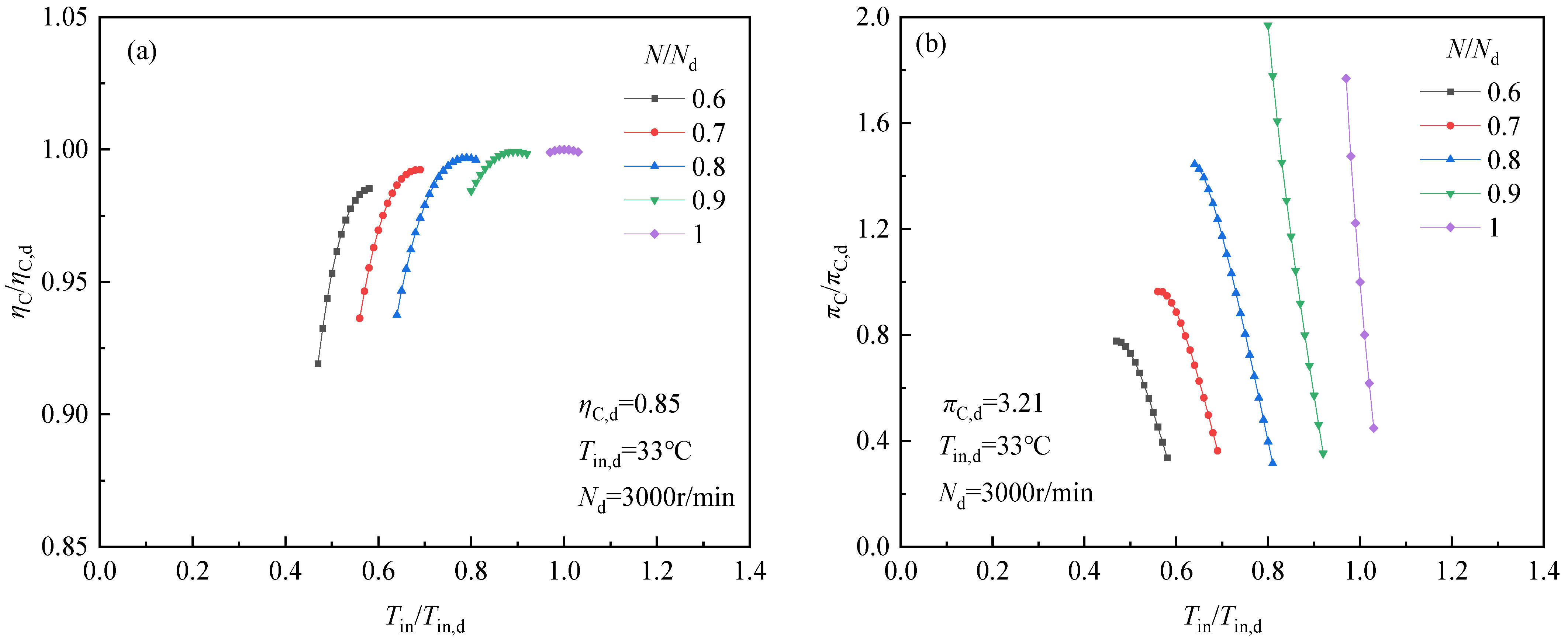
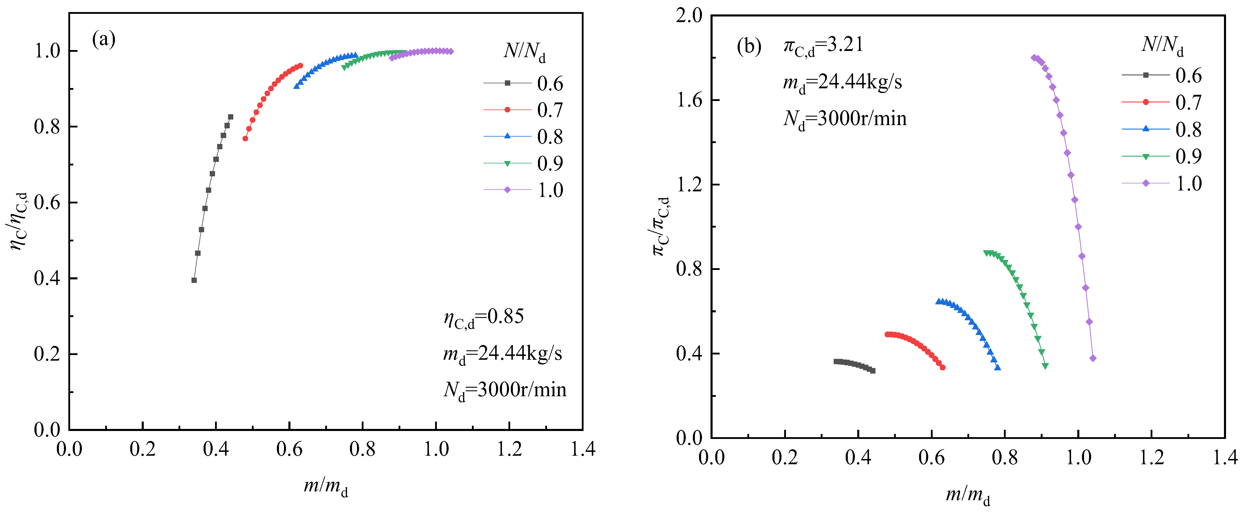
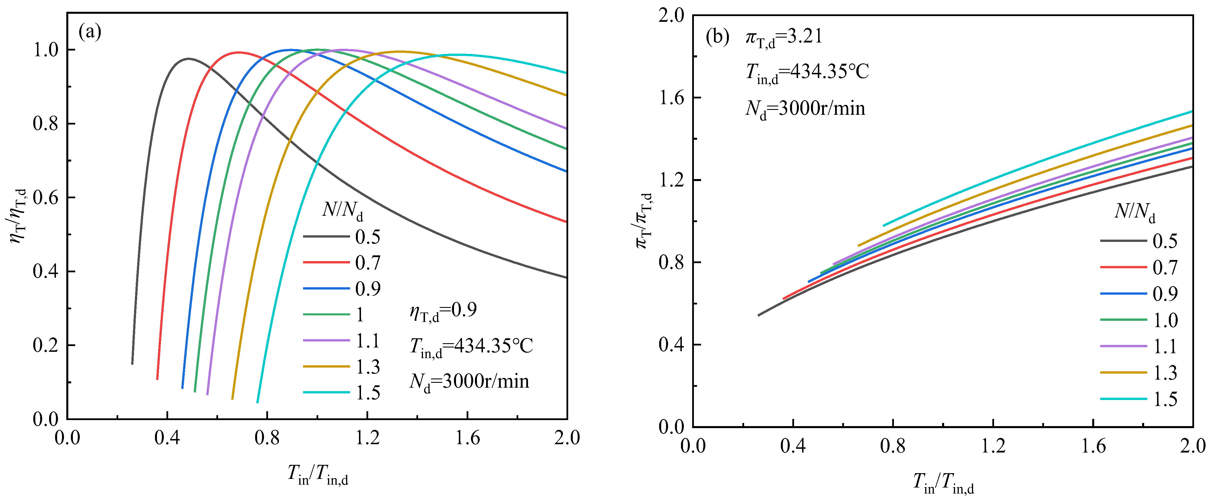
4.1. Modeling of Compressor

For compressors, the isentropic efficiency η_C under off-design conditions can be expressed by

$$\frac{{\eta }_{\mathrm{C}}}{{\eta }_{\mathrm{C},\mathrm{d}}}=\left[1-c_4\times {\left(1-\dot{N}\right)}^2\right]\left(\frac{\dot{N}}{\dot{m}}\right)(2-\frac{\dot{N}}{\dot{m}})$$

(18)

where η_C,d is the isentropic efficiency of the compressor under the design conditions, c₄ is the undetermined constant, which is generally set to be 0.3. Furthermore, $\dot{N}$ is the relative rotor speed of the compressor after correction, and $\dot{m}$ is the relative mass flow rate of the compressor after correction. They can be calculated by Equations (19) and (20), respectively.

$$\dot{N}=\frac{N}{N_{\mathrm{d}}}\sqrt{\frac{T_{\mathrm{in},\mathrm{d}}}{T_{\mathrm{in}}}}$$

(19)

where N is the actual rotor speed, N_d is the design rotor speed, T_in,d is the design inlet temperature of the compressor, and T_in is the actual inlet temperature of the compressor.

$$\dot{m}=\frac{m}{m_{\mathrm{d}}}\frac{P_{\mathrm{in},\mathrm{d}}}{P_{\mathrm{in}}}\sqrt{\frac{T_{\mathrm{in}}}{T_{\mathrm{in},\mathrm{d}}}}$$

(20)

where P_in,d is the designed inlet pressure of the compressor, and P_in is the actual inlet pressure of the compressor, m_d is the designed mass flow rate and m is the actual mass flow rate.

The relationship between the compression ratio of the compressor π_C and the relative mass flow rate $\dot{m}$ can be expressed as follows

$$\frac{{\pi }_{\mathrm{C}}}{{\pi }_{\mathrm{C},\mathrm{d}}}=c_1{\dot{m}}^2+c_2\dot{m}+c_3$$

(21)

where π_C is the actual compression ratio of the compressor, and π_C,d is the compression ratio of the compressor under the design conditions. c₁, c₂ and c₃ are related correction coefficients obtained by fitting empirical equations, which can be calculated as follows

$$c_1=\dot{N}/[p(1-q/\dot{N})+\dot{N}{(\dot{N}-q)}^2]$$

(22)

$$c_2=(p-2q{\dot{N}}^2)/[p(1-q/\dot{N})+\dot{N}{(\dot{N}-q)}^2]$$

(23)

$$c_3=-(pq\dot{N}-q^2{\dot{N}}^3)/[p(1-q/\dot{N})+\dot{N}{(\dot{N}-q)}^2]$$

(24)

where p and q are experimental parameters, and p and q are set to be 0.36 and 1.06, respectively, for large axial flow devices.

For compressors, the isentropic efficiency and compression ratio under off-design conditions can be determined by the corrected mass flow rate and rotor speed. Based on the above equations, the compressor model can be established to study the effects of relative mass flow rate and relative rotor speed on compressor performances. With the change in relative mass flow rate and relative rotor speed, the change curves of relative isentropic efficiency and relative compression ratio of the compressor are shown in Figure 5. m/m_d is in the range of 0.3 to 1.1, N/N_d is in the range of 0.6 to 1.0, η_C varies from 0 to 100%, and π_C is greater than 1.

When N/N_d of the compressor is 1 and m/m_d increases from 0.88 to 1.04, η_C/η_C,d of the compressor first increases from 0.98 to 1.00 and then decreases to 0.998, and π_C/π_C,d decreases from 1.8 to 0.37. As N/N_d of the compressor increases from 0.6 to 1.0, the relative isentropic efficiency curves shown in Figure 5a tend to flatten out, and the peak value of η_C/η_C,d and the corresponding m/m_d gradually increases. As shown in Figure 5b, as the ratio N/N_d increases, the relative compression ratio curves exhibit a tendency to steepen. Simultaneously, there is a gradual decrease in π_C/π_C,d, with their peak values and the corresponding m/m_d gradually increasing.

As shown in Figure 6, the relative inlet temperature and relative rotor speed have significant effects on compressor performances. The range of T_in/T_in,d is from 0.4 to 1.1, N/N_d is from 0.6 to 1.0, and η_C is from 0 to 100%. Furthermore, π_C/π_C,d is in the range of 0–2 and π_C is greater than 1. As can be seen from the figure where N/N_d is constant, with the increase in T_in/T_in,d, the η_C/η_C,d of the compressor increases rapidly at first, and then tends to be flat, while π_C/π_C,d decreases significantly. When the N/N_d of the compressor increases from 0.6 to 1.0, the relative isentropic efficiency curves tend to be flat. However, the decline trend of the relative compression ratio curves become steep with the increase in N/N_d.

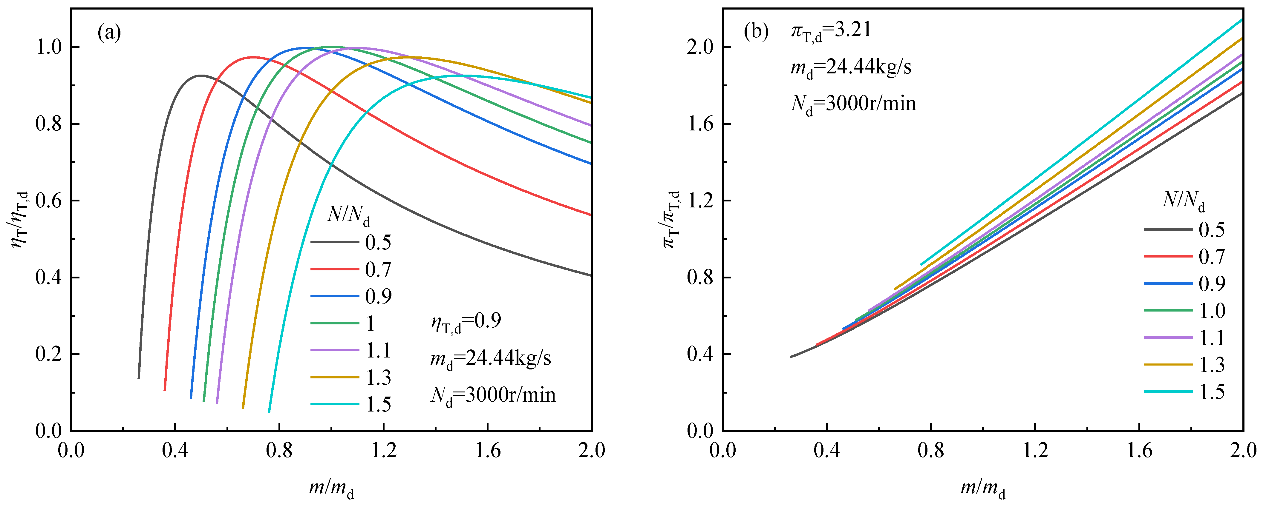
4.2. Modeling of Turbine

The isentropic efficiency η_T of the turbine under off-design conditions can be expressed by

$$\frac{{\eta }_{\mathrm{T}}}{{\eta }_{\mathrm{T},\mathrm{d}}}=\left[1-0.3{\left(1-\dot{N}\right)}^2\right]\left(\frac{\dot{N}}{\dot{m}}\right)(2-\frac{\dot{N}}{\dot{m}})$$

(25)

where η_T,d is the isentropic efficiency of the turbine under the design conditions, $\dot{N}$ is the relative rotor speed of the turbine after correction, $\dot{m}$ is the relative mass flow rate of the turbine after correction, and their calculation methods are the same as those of the compressor.

Furthermore, the mass flow rate m, rotor speed N, inlet temperature T_in and expansion ratio π_T of the turbine are mutually constrained, and the corresponding coupling relationship can be expressed as follows:

$$\frac{m}{m_{\mathrm{d}}}=\sqrt{1.4-0.4\frac{N}{N_{\mathrm{d}}}}\sqrt{\frac{T_{\mathrm{in}}}{T_{\mathrm{in},\mathrm{d}}}}\sqrt{\frac{({{\pi }_{\mathrm{T}}}^2-1)}{({{\pi }_{\mathrm{T},\mathrm{d}}}^2-1)}}$$

(26)

where π_T is the actual expansion ratio of the turbine, and π_T,d is the expansion ratio of the turbine under the design conditions.

Based on the above control equations, the effects of relative mass flow rate and relative rotor speed on turbine performances are studied. The effects of m/m_d on the turbine relating to relative isentropic efficiency and the relative expansion ratio of the turbine are shown in Figure 7. The range of m/m_d is from 0.0 to 2.0, N/N_d is from 0.5 to 1.5, η_T is from 0 to 100%, and π_T is greater than 1. It can be seen that when N/N_d is 1 and m/m_d increases from 0.51 to 2.0, η_T/η_T,_d increases rapidly from 0.077 to 1, and then slowly decreases to 0.75, while π_T/π_T,_d increases from 0.576 to 1.926. When the N/N_d of the turbine increases from 0.5 to 1.5, the peak value of η_T/η_T,_d gradually increases from 0.925 to the maximum value 1 initially and then decreases to 0.925, while its corresponding m/m_d gradually increases, and the relative expansion ratio curves become steep. Furthermore, when the m/m_d of the turbine is 1 and N/N_d increases from 0.5 to 1.5, η_T/η_T,_d is symmetric with respect to N/N_d = 1, increasing from 0.694 to 1.00 and then decreasing to 0.694, while π_T/π_T,_d increases from 0.922 to 1.107.

As shown in Figure 8, relative inlet temperature and relative rotor speed have significant effects on the isentropic efficiency and expansion ratio of the turbine. The range of T_in/T_in,d is from 0.0 to 2.0, and the ranges of N/N_d, η_T and π_T are the same as those in Figure 7. When the N/N_d of the turbine is constant, with the increase in T_in/T_in,d, η_T/η_T,d increases rapidly and then decreases slowly, while π_T/π_T,d increases steadily. When N/N_d increases from 0.5 to 1.5, the peak value of η_T/η_T,d remains basically unchanged, which increases from 0.975 to 1 and then decreases to 0.986, while the relative expansion ratio curves increase slowly.

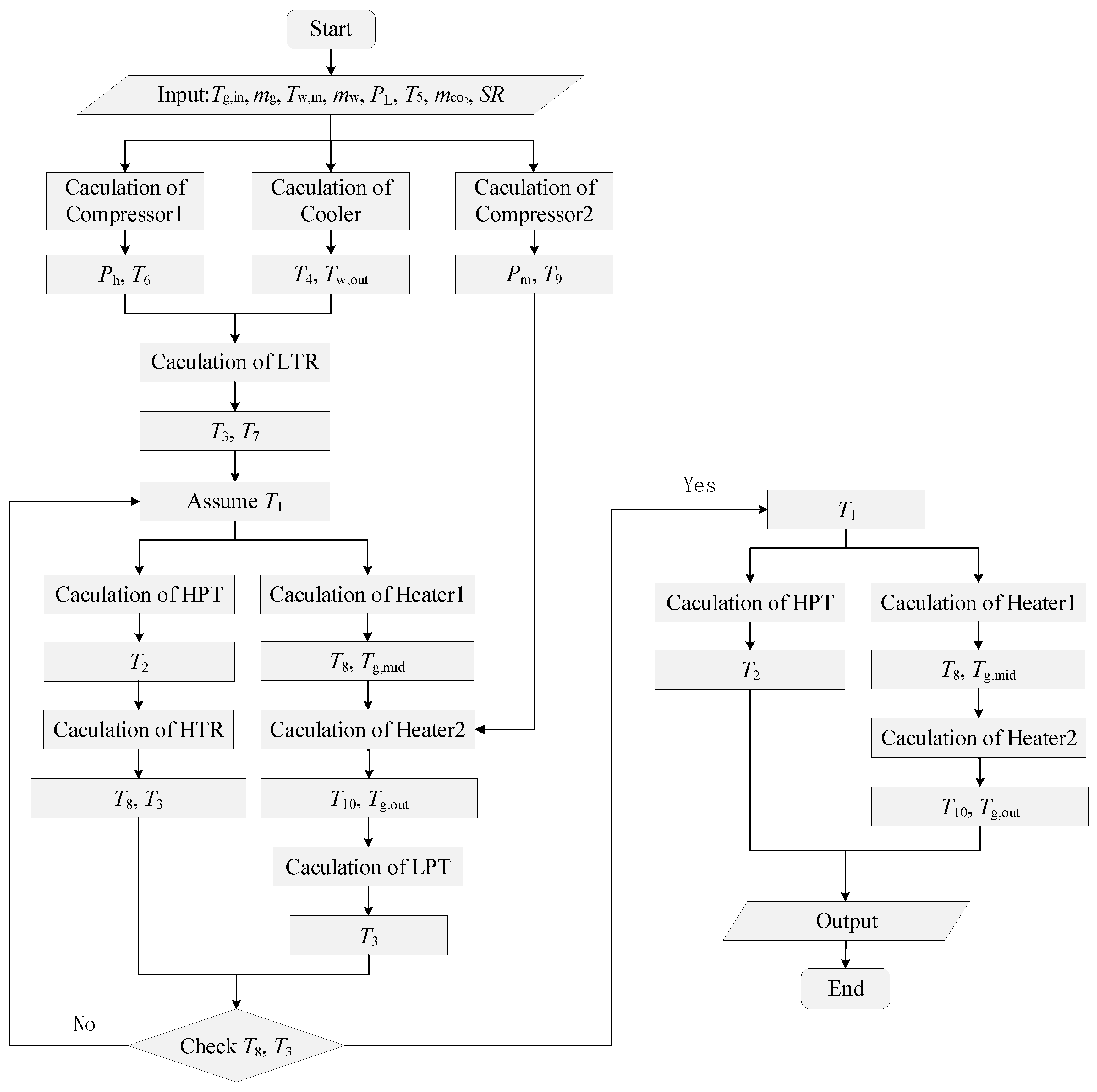
5. Off-Design Performance Calculation of S-CO₂ Cycle

Based on the above solution methods of the system components, the off-design working condition models of the compressor, turbine and heat exchangers are programmed on the Matlab platform. In addition, the physical properties of CO₂, flue gas and water can be calculated by the REFPROP 9.0 software, based on known parameters. The corresponding calculation flow of the S-CO₂ power cycle under off-design working conditions is established, as shown in Figure 9. Firstly, the parameters, such as cold and heat source conditions, compressor inlet temperature and pressure, the mass flow rates of the working fluids and split ratio, are input. Then the models of the cooler, compressors, recuperators, turbines and heaters are calculated successively. Finally, the parameters of each state point are output, and the cycle performance parameters such as the net output work and cycle efficiency can be obtained.

6. Effects of Key System Parameters

During industrial production, cold and heat source parameters often fluctuate, which can impact the output parameters of system components and the performance of the cycle. In order to evaluate the system performances under off-design conditions, we analyze the cycle performances by controlling key variables such as cooling water inlet temperature, cooling water mass flow rate, flue gas inlet temperature and flue gas mass flow rate.

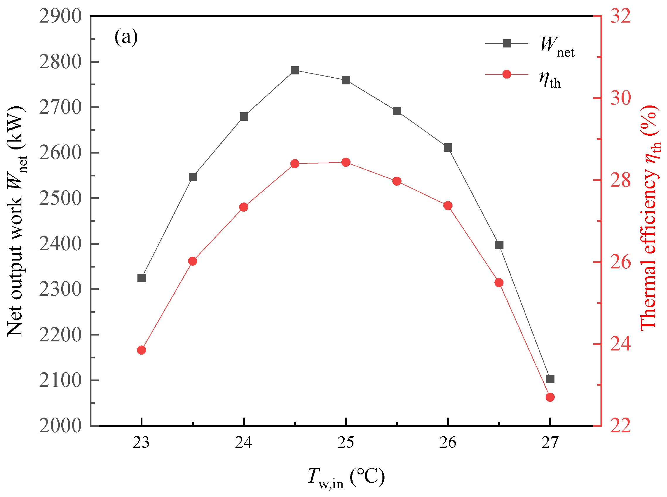
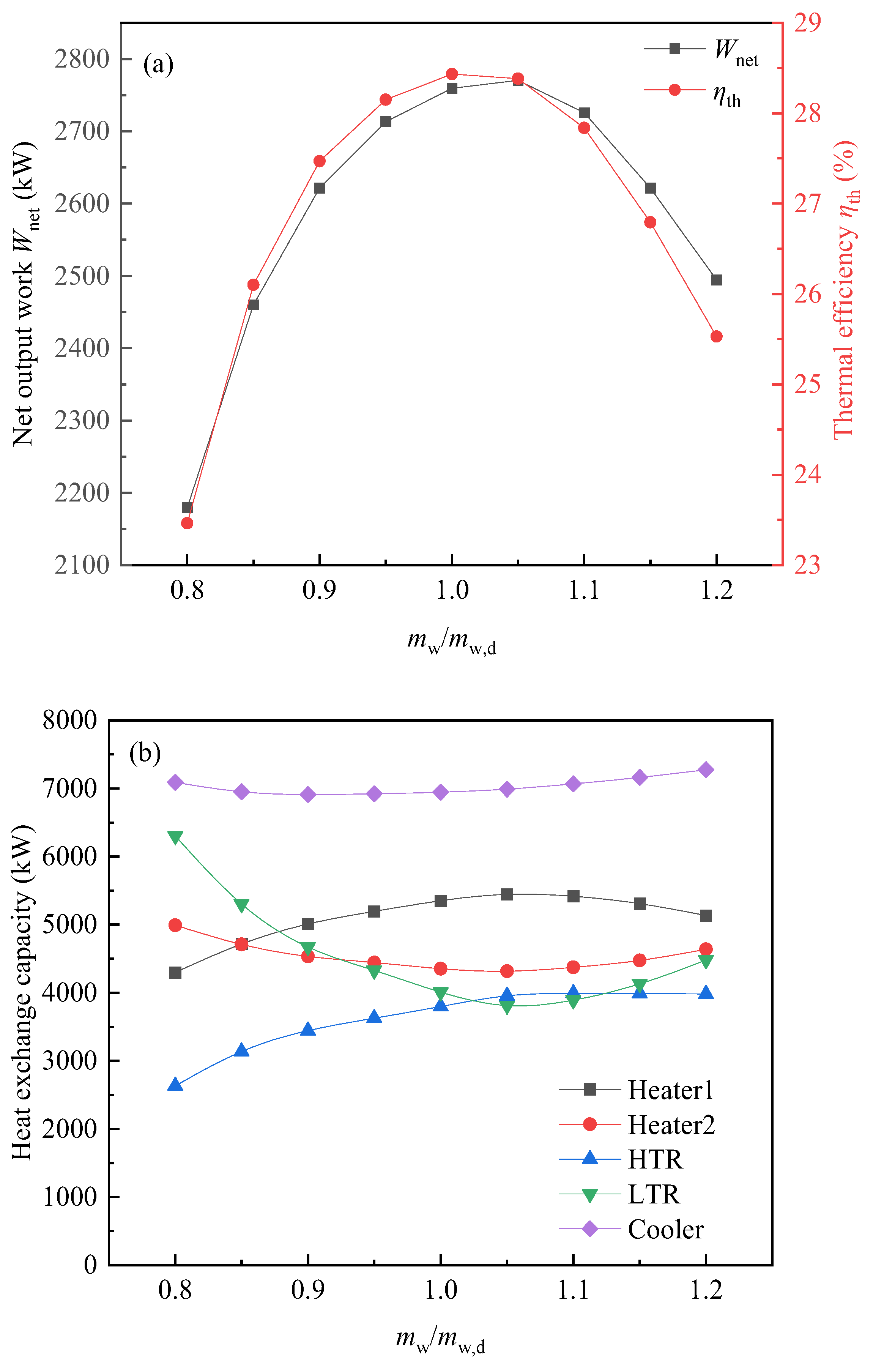
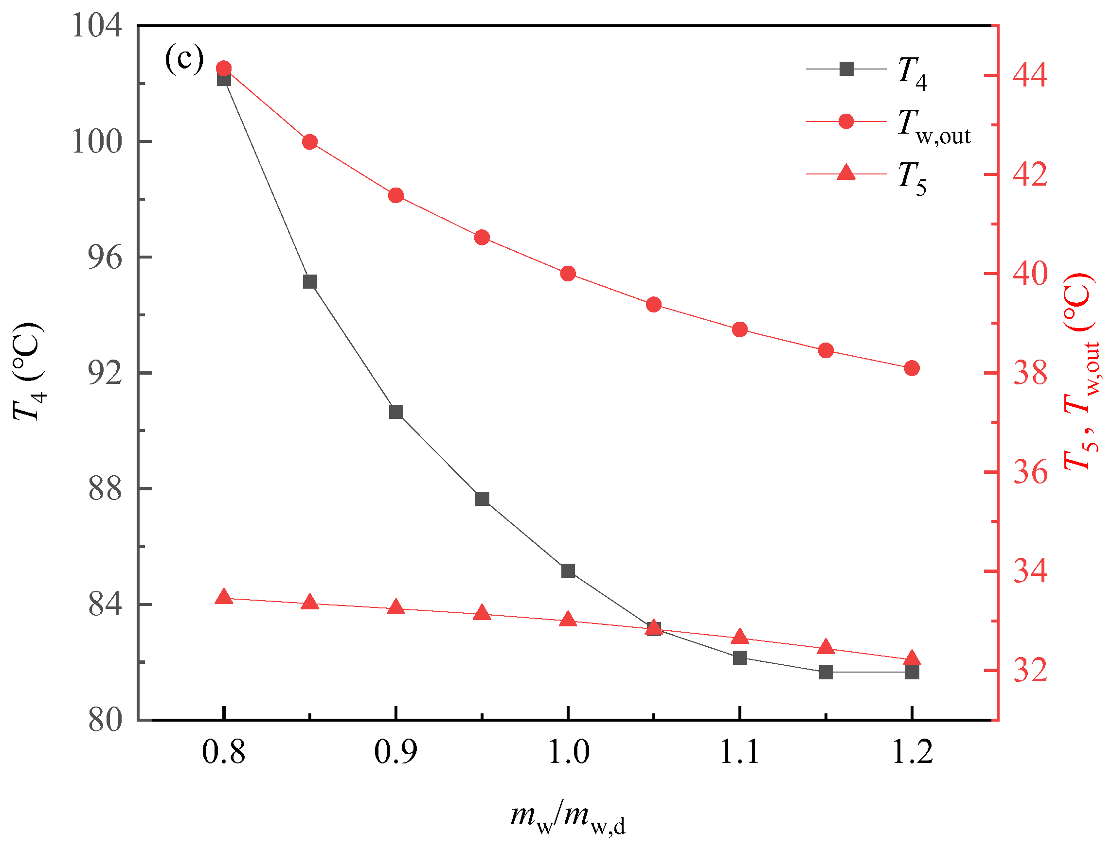
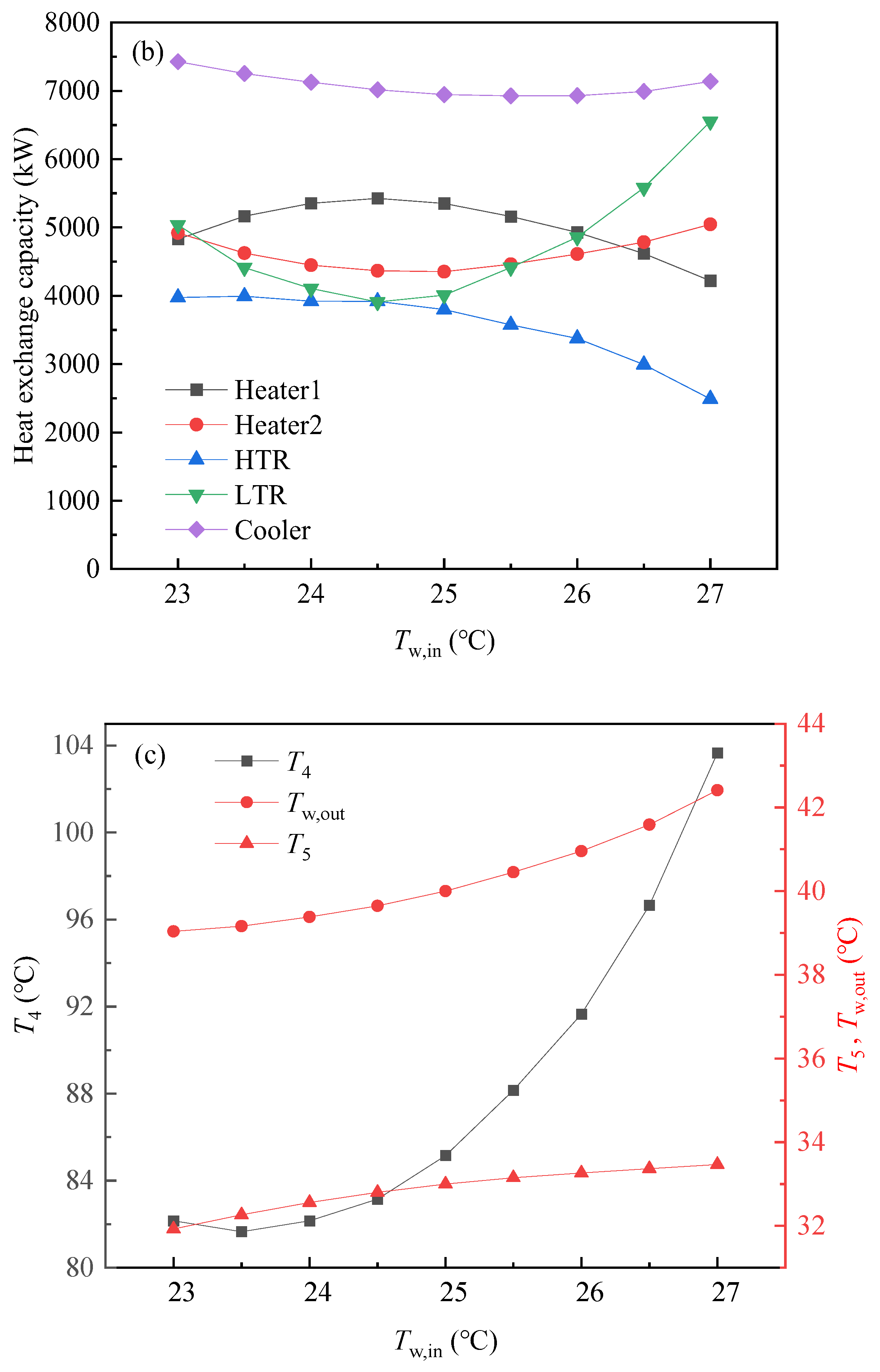
6.1. Effects of Cold Source Parameters

For the S-CO₂ power cycle that recovers flue gas waste heat, the cooling method is generally water cooling. In the actual production, the temperature of the cooling water is easily affected by the ambient temperature. Therefore, it is of practical significance to study the effects of cooling water parameters on the off-design characteristics of the system [34].

Under off-design conditions, the effects of cooling water inlet temperature on the system performances are analyzed when the other parameters are constant. As shown in Figure 10, the inlet temperature of the cooling water under the design working conditions is 25 °C, and the variation range of the inlet temperature is set at 23–27 °C. As the inlet temperature of the cooling water increases, the outlet temperature of the cooling water increases, and the inlet temperature T₄ and outlet temperature T₅ of the CO₂ side of the cooler gradually increase. As can be seen from Figure 6, the variation in the compressor inlet temperature has a weak effect on the isentropic efficiency, while it has a drastic effect on the compression ratio. Thus, the compression ratio gradually decreases as the compressor inlet temperature increases. With the increase in T₅ and the decrease in compressor outlet pressure, the compressor outlet temperature T₆ and T₉ increase correspondingly, and the compression work decreases first and then increases.

As the CO₂ inlet temperature T₉ of Heater2 gradually increases, there is an initial decrease followed by an increase in outlet temperature T₁₀. The heat absorption in Heater2 also follows a similar trend, with the heat absorption first decreasing and then increasing as the inlet temperature slowly changes. When the CO₂ inlet temperature T₈ of Heater1 decreases first and then increases, the flue gas outlet temperature and CO₂ outlet temperature T₁ decreases first and then increases, while the flue gas inlet temperature remains constant. Consequently, the heat absorption in Heater1 initially increases but subsequently decreases.

From Figure 8a, it can be seen that the isentropic efficiency decreases as the turbine inlet temperature deviates from the design value at constant rotor speed. As shown in Figure 8b, due to the gradual decrease in the inlet pressure of the turbine, the rotor speed of the turbine is gradually reduced in order to maintain a stable low outlet pressure, resulting in a corresponding decrease in isentropic efficiency. Due to the effects of inlet temperature and rotor speed, both the outlet temperatures T₂ and T₃ of the turbines initially decrease and then increase, while total expansion work first increases and then decreases. Consequently, the net output work of the system increases from 2324.41 kW to 2781.11 kW and then decreases to 2102.63 kW. The total heat absorbed from the flue gas heat source follows the trend of initially increasing and subsequently decreasing, leading to an improvement in thermal efficiency from 23.85% to 28.43%, followed by a decline to 22.69%.

The impacts of the cooling water mass flow rate on the system’s performance characteristics under off-design conditions are illustrated in Figure 11. The cooling water mass flow rate varies within the range of 0.8–1.2 times the design value. Within this investigated range, the CO₂ inlet and outlet temperatures T₄ and T₅ of the cooler gradually decrease as the cooling water mass flow rate increases. Simultaneously, there is a gradual decrease in compressor outlet temperatures T₆ and T₉, an increase in compressor outlet pressure, and a non-linear trend observed for total compression work with an initial decrease followed by an increase. Furthermore, the CO₂ outlet temperature T₁₀ of the Heater2 exhibits a similar trend of first decreasing and then increasing. Compared to T₉, the variation in T₁₀ is much greater, resulting in a fluctuating heat absorption for Heater2, characterized by an initial decrease followed by an increase. For Heater1, the flue gas outlet temperature T_g,mid initially decreases and then increases while maintaining a constant flue gas inlet temperature. Therefore, the heat absorption first increases and then decreases.

As the medium and high pressures at the turbine inlet gradually increase, the turbine rotor speed gradually increases in order to keep the low pressure constant. Meanwhile, the isentropic efficiency and the total expansion work first increase and then decrease. Thus, the net output work of the system rises from 2179.45 kW to 2770.51 kW and then declines to 2494.5 kW. The total heat absorbed from the flue gas heat source experiences a slow increase followed by a decrease. As a result, the thermal efficiency increases from 23.46% to 28.43% and then decreases to 25.53%.

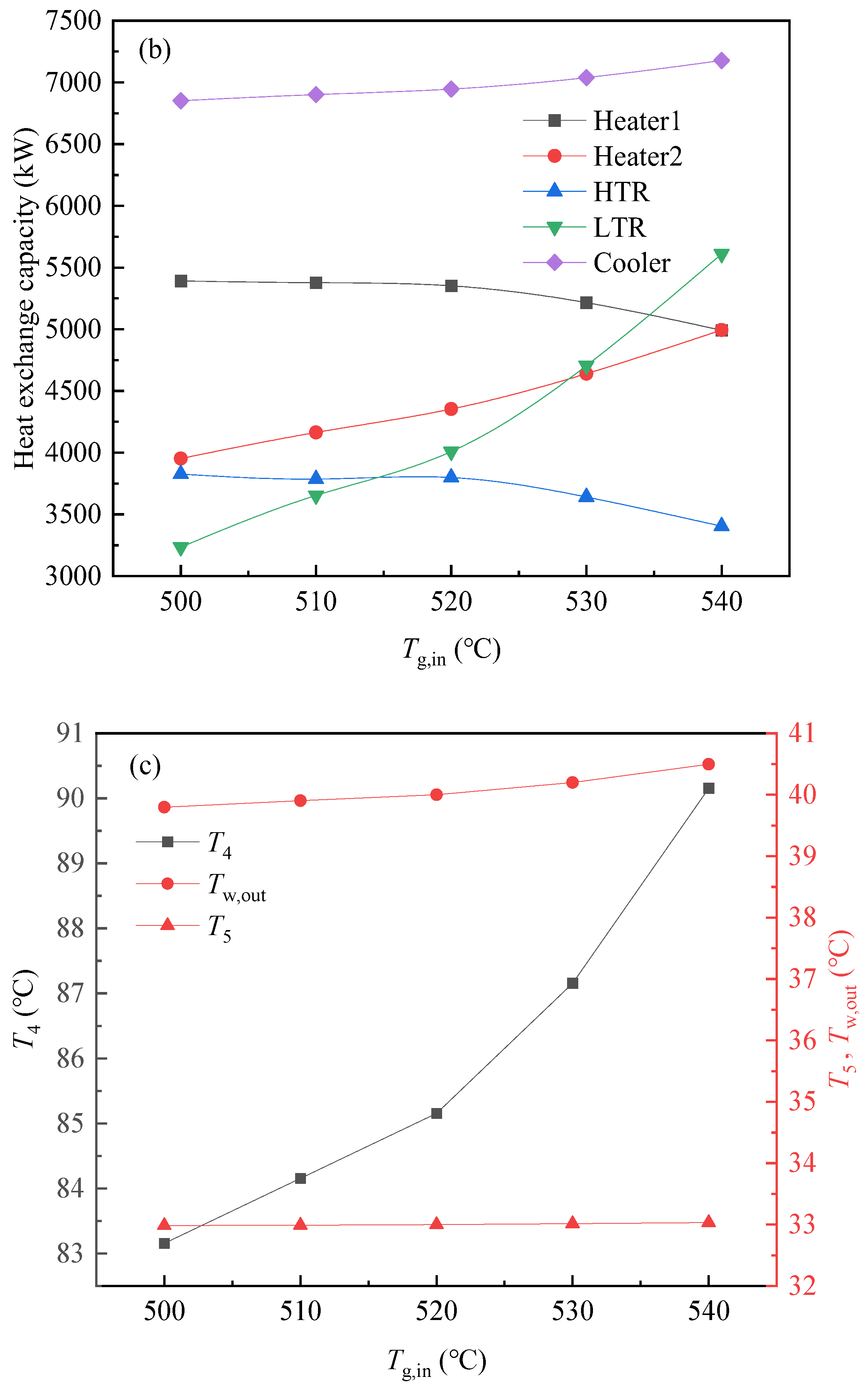
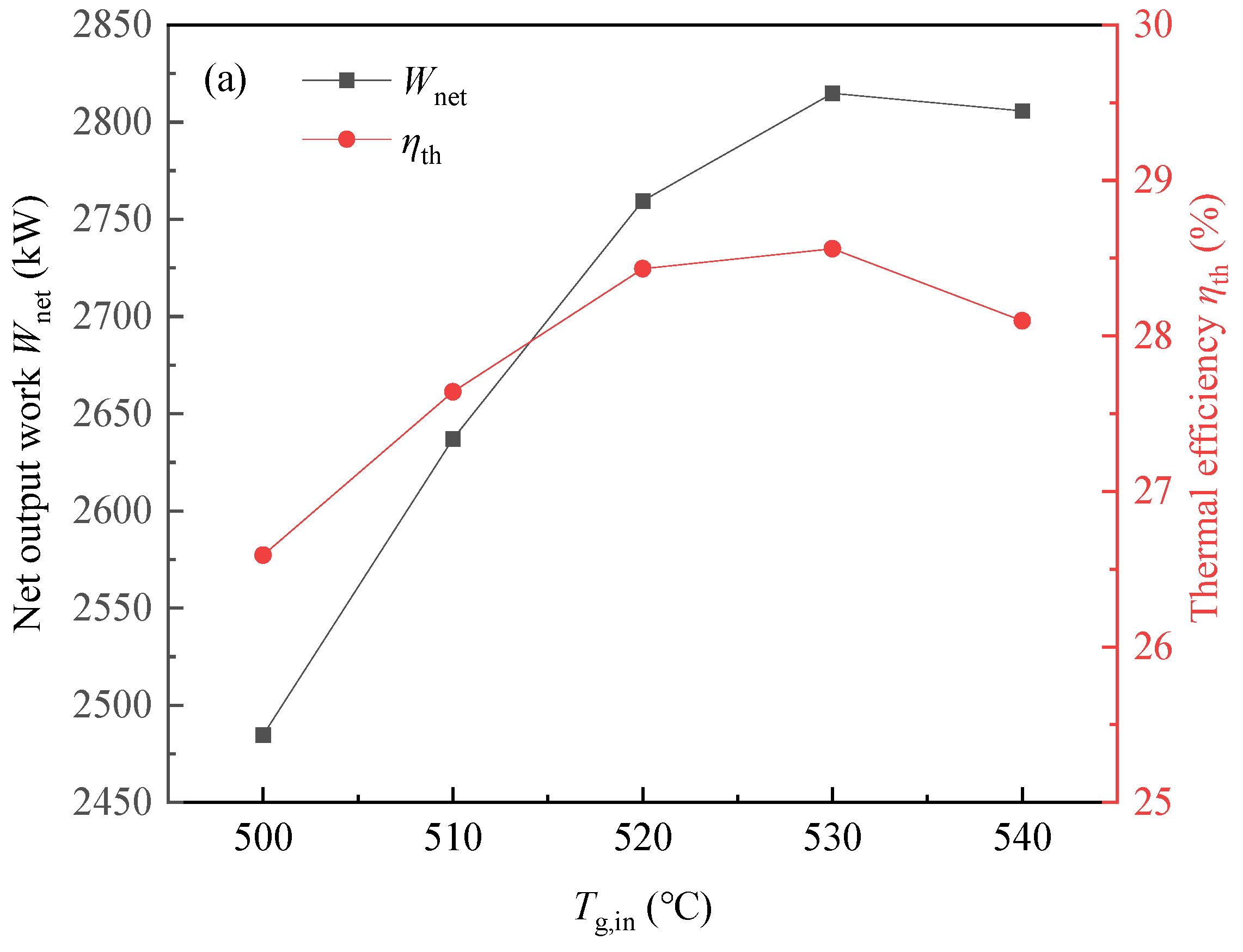
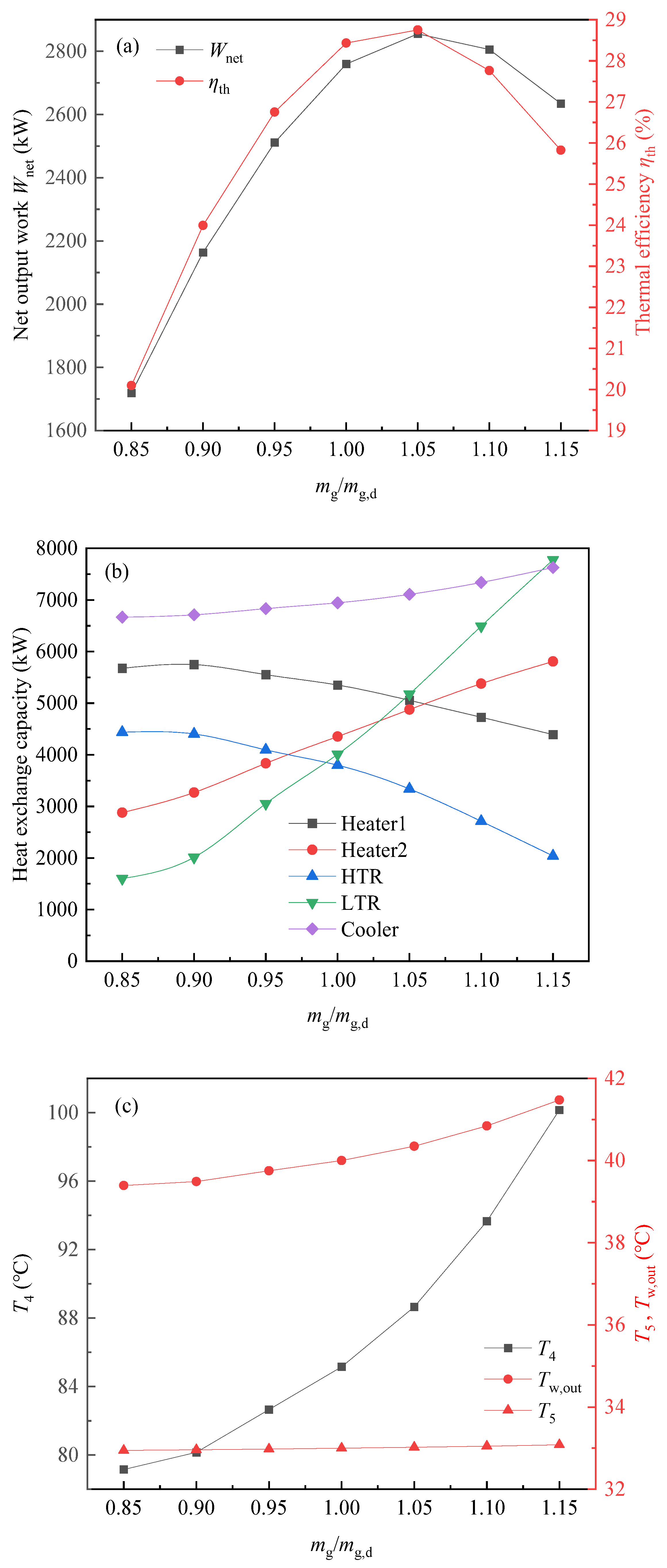
6.2. Effects of Heat Source Parameters

The impacts of the flue gas inlet temperature on the system performances under off-design conditions can be observed in Figure 12. With the flue gas inlet temperature T_g,in increasing, both the flue gas outlet temperature T_g,mid of Heater1 and T_g,out of Heater2 gradually rise. As T_g,mid increases faster than T_g,in and T_g,out, the heat absorption in Heater1 gradually decreases while the heat absorption in Heater2 gradually increases.

The HPT inlet temperature T₁ rises with the flue gas inlet temperature, resulting in a corresponding gradual increase in expansion work. Similarly, the LPT inlet temperature T₁₀ increases with the flue gas outlet temperature of Heater1, leading to an increase in the turbine outlet temperature T₃, and consequently the expansion work initially increases before decreasing.

Due to the small variations in compressor inlet and outlet temperatures, the compression work is less affected by the flue gas inlet temperature. Therefore, the net output work of the system increases from 2484.67 kW to 2814.88 kW, and then decreases to 2805.83 kW. The total heat absorbed from the flue gas heat source gradually increases, resulting in a rise in thermal efficiency from 26.59% to 28.56%, followed by a decrease to 28.1%.

The effects of the flue gas mass flow rate on the system performances under off-design conditions are depicted in Figure 13, with other input parameters held constant. The flue gas mass flow rate varies within the range of 0.85–1.15 times the design value. As the flue gas mass flow rate increases, the flue gas outlet temperatures of Heater1 and Heater2 gradually increase. However, as the flue gas inlet temperature remains constant, the overall heat absorption of Heater1 shows a decreasing trend. Furthermore, considering that the flue gas inlet temperature of Heater2 increases more rapidly than the outlet temperature, the heat absorption of Heater2 gradually increases.

The inlet temperature T₁ of the HPT rises with the increase in flue gas mass flow rate, leading to an increase and then a decrease in expansion work. Similarly, the inlet temperature T₁₀ of the LPT increases with the increase in the flue gas outlet temperature of Heater1, resulting in an initial increase followed by a decrease in expansion work.

Given the slight changes in the compressor inlet and outlet temperatures, the compression work is less affected by the flue gas mass flow rate. Therefore, the net output work of the system increases from 1719.01 kW to 2855.09 kW and then decreases to 2634.58 kW. Furthermore, the total heat absorbed gradually increases, leading to an increase in thermal efficiency from 20.1% to 28.75%, followed by a decrease to 25.83%.

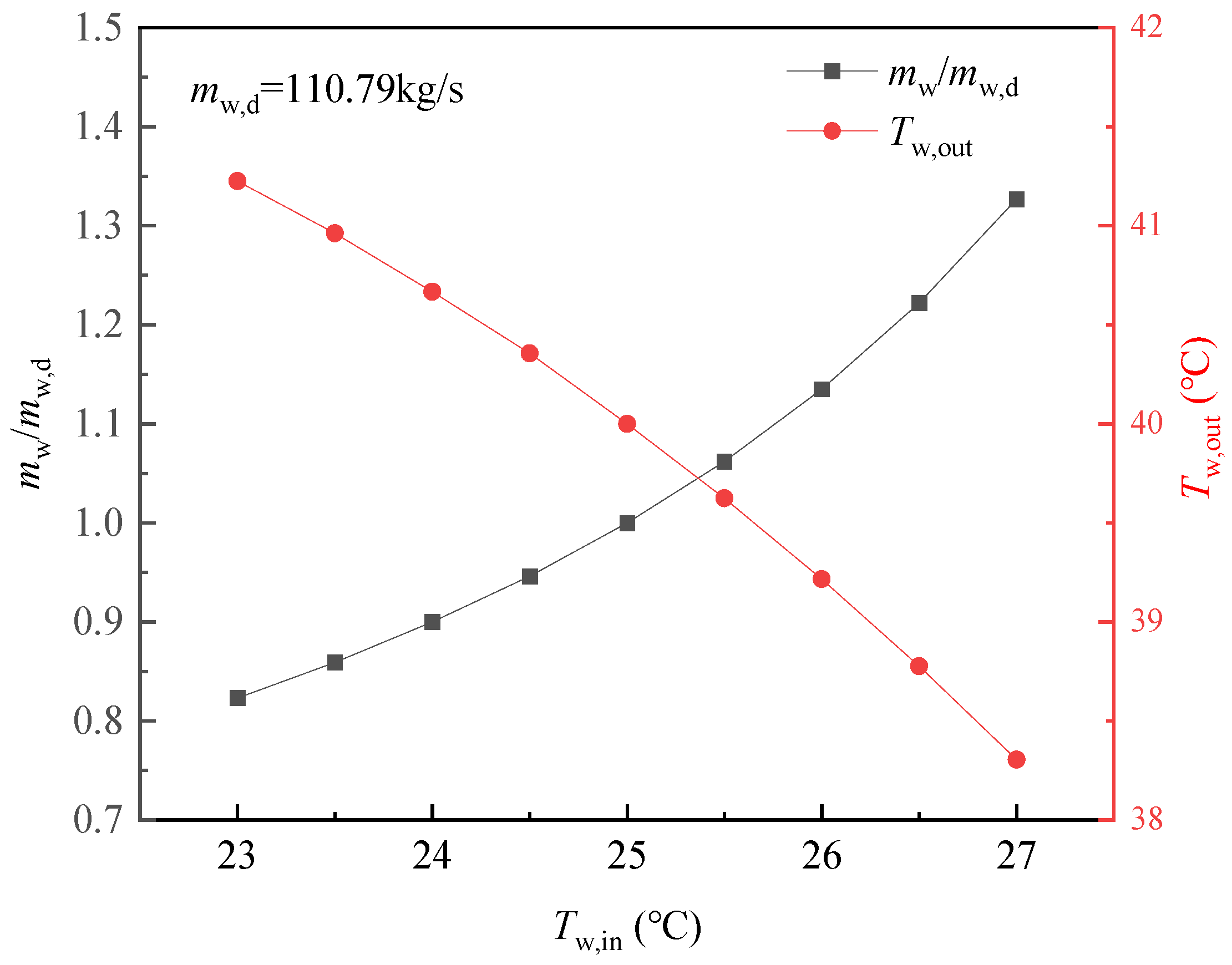
7. Control Strategy of the Cooling Process

Based on the above analysis, it can be seen that the inlet temperature and mass flow rate of cooling water have great effects on the system performance. When the inlet temperature of the cooling water increases from 23 °C to 27 °C, compared with the optimal value, the net output work of the cycle decreases by up to 24.4% and the cycle thermal efficiency decreases by up to 20.19%. In actual production, the cooling water inlet temperature is easily affected by natural environmental conditions, and the compressor performance is significantly affected by the cooling water inlet temperature, thus affecting the overall performances of the system. Therefore, when the inlet temperature of the cooling water fluctuates, in order to ensure the efficient and stable operation of the system, it is necessary to develop the corresponding control strategy.

Compared with regulating the flue gas inlet temperature and flue gas mass flow rate, it is more convenient to adjust the cooling water mass flow rate to reduce the effect of the cooling water inlet temperature on the system. Meanwhile, it has less effect on other parameters of the system, and it is easy to operate in actual production. Therefore, the effect of the cooling water inlet temperature is controlled by regulating the cooling water mass flow rate.

By changing the cooling water mass flow rate, the temperature changes on the CO₂ side of the cooler can be attenuated. In this paper, the CO₂ outlet temperature T₅ of the cooler is set to the design value, and the range of the cooling water mass flow rate is set based on the design value. The optimal value can be found by the exhaustive method to make T₄ closer to the design value. Based on the cooling water mass flow rate control strategy, the parameter changes in the cooler are shown in Figure 14. In order to make the parameters on the CO₂ side closer to the design values, when the inlet temperature of cooling water increases from 23 °C to 27 °C, the mass flow rate of the cooling water will increase from 82.3% to 132.7% of the design value, and the outlet temperature of the cooling water will decrease from 41.23 °C to 38.3 °C.

8. Conclusions

In this paper, the thermal performance and control strategy of an innovative S-CO₂ power cycle driven by flue gas waste heat are investigated under off-design conditions. According to the design parameters of the S-CO₂ cycle, the off-design models of system components including the turbine, compressor, printed circuit heat exchangers and shell-and-tube heat exchangers are first established. Then, under off-design conditions, performance characteristics of the system are analyzed and discussed. Finally, aiming at the S-CO₂ cooling process, the control strategy of the cooling water flow is proposed to match the inlet temperature variation in cooling water. The main conclusions can be drawn as follows:

(1) When the inlet temperature and mass flow rate of the cooling water change, the cycle efficiency can reach the maximum value of 28.43% at the design point. When the flue gas inlet temperature changes, the maximum cycle efficiency 28.56% is obtained at 530 °C. For the variation of the flue gas mass flow rate, at the mass flow ratio 1.05, the cycle efficiency reaches the peak of 28.75%.

(2) To ensure the efficient and stable operation of the S-CO₂ power cycle, a control strategy of the cold end is proposed for the inlet temperature variation in the cooling water. When the cooling water inlet temperature increases from 23 °C to 27 °C, the cooling water mass flow rate should increase from 82.3% to 132.7% of the design value.

Based on the research in this paper, more control strategies will be studied in the future so as to deal with different changes in working conditions, such as flue gas parameter variations and rotational speed variations. In addition, the dynamic characteristics of the S-CO₂ cycle will be further investigated to reveal the parameter variations in the system under full operating conditions. On this basis, relevant control methods will be proposed to guide the operation of a practical engineering system.

References

1. Chen, S.; Zheng, Y.; Wu, M.; Hu, J.; Xiang, W. Thermodynamic analysis of oxy-fuel combustion integrated with the sCO2 Brayton cycle for combined heat and power production. Energy Convers. Manag. 2021, 232, 113869. [Google Scholar] [CrossRef]
2. Kareem, P.H.; Ali, M.; Tursoy, T.; Khalifa, W. Testing the Effect of Oil Prices, Ecological Footprint, Banking Sector Development and Economic Growth on Energy Consumptions: Evidence from Bootstrap ARDL Approach. Energies 2023, 16, 3365. [Google Scholar] [CrossRef]
3. Wang, X.; Zhang, M. The Thermal Economy of a Circulating Medium and Low Temperature Waste Heat Recovery System of Industrial Flue Gas. Int. J. Heat Technol. 2021, 39, 1680–1688. [Google Scholar] [CrossRef]
4. Gao, B.; Sun, Z. Marginal CO2 and SO2 Abatement Costs and Determinants of Coal-Fired Power Plants in China: Considering a Two-Stage Production System with Different Emission Reduction Approaches. Energies 2023, 16, 3488. [Google Scholar] [CrossRef]
5. Larjola, J. Electricity from industrial waste heat using high-speed organic Rankine cycle (ORC). Int. J. Prod. Econ. 1995, 41, 227–235. [Google Scholar] [CrossRef]
6. Wang, E.; Peng, N. A Review on the Preliminary Design of Axial and Radial Turbines for Small-Scale Organic Rankine Cycle. Energies 2023, 16, 3423. [Google Scholar] [CrossRef]
7. Loni, R.; Najafi, G.; Bellos, E.; Rajaee, F.; Mazlan, M. A review of industrial waste heat recovery system for power generation with Organic Rankine Cycle: Recent Challenges and Future Outlook. J. Clean. Prod. 2020, 287, 125070. [Google Scholar] [CrossRef]
8. Carrillo Caballero, G.; Cardenas Escorcia, Y.; Venturini, O.J.; Silva Lora, E.E.; Alviz Meza, A.; Mendoza Castellanos, L.S. Unidimensional and 3D Analyses of a Radial Inflow Turbine for an Organic Rankine Cycle under Design and Off-Design Conditions. Energies 2023, 16, 3383. [Google Scholar] [CrossRef]
9. Zhang, R.; Su, W.; Lin, X.; Zhou, N.; Zhao, L. Thermodynamic analysis and parametric optimization of a novel S–CO2 power cycle for the waste heat recovery of internal combustion engines. Energy 2020, 209, 118484. [Google Scholar] [CrossRef]
10. Guo, J.; Li, M.; He, Y.; Jiang, T.; Ma, T.; Xu, J.; Cao, F. A systematic review of supercritical carbon dioxide(S-CO2) power cycle for energy industries: Technologies, key issues, and potential prospects. Energy Convers. Manag. 2022, 258, 115437. [Google Scholar] [CrossRef]
11. Yu, A.; Xing, L.; Su, W.; Liu, P. State-of-the-art review on the CO2 combined power and cooling system: System configuration, modeling and performance. Renew. Sustain. Energy Rev. 2023, 188, 113775. [Google Scholar] [CrossRef]
12. White, M.T.; Bianchi, G.; Chai, L.; Tassou, S.A.; Sayma, A.I. Review of supercritical CO2 technologies and systems for power generation. Appl. Therm. Eng. 2021, 185, 116447. [Google Scholar] [CrossRef]
13. Liang, Y.; Lin, X.; Su, W.; Xing, L.; Zhou, N. Thermal-economic analysis of a novel solar power tower system with CO2-based mixtures at typical days of four seasons. Energy 2023, 276, 127602. [Google Scholar] [CrossRef]
14. Rahbari, H.R.; Mandø, M.; Arabkoohsar, A. A review study of various High-Temperature thermodynamic cycles for multigeneration applications. Sustain. Energy Technol. Assess. 2023, 57, 103286. [Google Scholar] [CrossRef]
15. Liao, J.; Liu, X.; Zheng, Q.; Zhang, H. Analysis of supercritical CO2 power generation cycle characteristics. Therm. Power Eng. 2016, 31, 40−46+149−150. [Google Scholar] [CrossRef]
16. Fang, Z.; Dong, X.; Tang, X. Research on gas engine waste heat recovery system based on S-CO2. Combust. Sci. Technol. 2023, 29, 543–551. [Google Scholar]
17. Fu, J. Research on Optimization of Supercritical Carbon Dioxide Brayton Cycle Thermodynamic System. Master’s Thesis, North China Electric Power University, Beijing, China, 2020. [Google Scholar]
18. Lock, A.; Bone, V. Off-design operation of the dry-cooled supercritical CO2 power cycle. Energy Convers. Manag. 2022, 251, 114903. [Google Scholar] [CrossRef]
19. Duniam, S.; Veeraragavan, A. Off-design performance of the supercritical carbon dioxide recompression Brayton cycle with NDDCT cooling for concentrating solar power. Energy 2019, 187, 115992. [Google Scholar] [CrossRef]
20. Xiao, G.; Yu, A.; Lin, X.; Su, W.; Zhou, N. Constructing a novel supercritical carbon dioxide power cycle with the capacity of process switching for the waste heat recovery. Int. J. Energy Res. 2022, 46, 5099–5118. [Google Scholar] [CrossRef]
21. Wu, C.; Wang, S.-S.; Bai, K.-L.; Li, J. Thermodynamic analysis and parametric optimization of CDTPC-ARC based on cascade use of waste heat of heavy-duty internal combustion engines (ICEs). Appl. Therm. Eng. 2016, 106, 661–673. [Google Scholar] [CrossRef]
22. Huang, J.; Han, Z.; Guo, J.; Huai, X. Research progress of supercritical CO2 microchannel heat exchangers. J. Refrig. 2023, 44, 1–14. [Google Scholar]
23. Rao, Z.; Xue, T.; Huang, K.; Liao, S. Multi-objective optimization of supercritical carbon dioxide recompression Brayton cycle considering printed circuit recuperator design. Energy Convers. Manag. 2019, 201, 112094. [Google Scholar] [CrossRef]
24. Wang, Z.; Zhu, Y.; Wang, F.; Wang, P.; Liu, J. In Proceedings of the 11th International Symposium on Heating, Ventilation and Air Conditioning (ISHVAC 2019): Volume III: Buildings and Energy; Springer: Berlin/Heidelberg, Germany, 2020.
25. Ngo, T.L.; Kato, Y.; Nikitin, K.; Tsuzuki, N. New printed circuit heat exchanger with S-shaped fins for hot water supplier. Exp. Therm. Fluid Sci. 2006, 30, 811–819. [Google Scholar] [CrossRef]
26. Gnielinski, V. New equations for heat and mass transfer in the turbulent flow in pipes and channels. In NASA STI/Recon Technical Report A; NASA/ADS: Washington, DC, USA, 1975; Volume 41. [Google Scholar]
27. Dittus, F.W.; Boelter, L.M.K. Heat transfer in automobile radiators of the tubular type. Int. Commun. Heat Mass Transf. 1985, 12, 3–22. [Google Scholar] [CrossRef]
28. Zhang, Z.; Liu, J.; Wang, S.; Zheng, W. Thermodynamic calculation and numerical simulation of shell-and-tube heat exchangers. Non-Ferr. Metall. Energy Effic. 2012, 28, 34−38+28. [Google Scholar]
29. Tun, C.M.; Fane, A.G.; Matheickal, J.T.; Sheikholeslami, R. Membrane distillation crystallization of concentrated salts-Flux and crystal formation. J. Membr. Sci. 2005, 257, 144–155. [Google Scholar] [CrossRef]
30. Qi, F. Advances in heat transfer calculation methods for shell-and-shell heat exchangers without phase change. Pharm. Eng. 2002, 23, 29–36. [Google Scholar]
31. Jeong, Y.; Son, S.; Cho, S.K.; Baik, S.; Lee, J.I. Evaluation of supercritical CO2 compressor off-design performance prediction methods. Energy 2020, 213, 119071. [Google Scholar] [CrossRef]
32. Wang, W.; Cai, R.; Zhang, N. General characteristics of single shaft microturbine set at variable speed operation and its optimization. Appl. Therm. Eng. 2004, 24, 1851–1863. [Google Scholar] [CrossRef]
33. Zhang, N.; Cai, R. Analytical solutions and typical characteristics of part-load performance of single shaft gas turbine and its cogeneration. Energy Convers. Manag. 2002, 43, 1323–1337. [Google Scholar] [CrossRef]
34. Poškas, R.; Sirvydas, A.; Kulkovas, V.; Poškas, P.; Jouhara, H.; Miliauskas, G.; Puida, E. Flue Gas Condensation in a Model of the Heat Exchanger: The Effect of the Cooling Water Flow Rate and Its Temperature on Local Heat Transfer. Appl. Sci. 2022, 12, 12650. [Google Scholar] [CrossRef]
Figure 1. Layout diagram of the system.
Energies 17 01871 g001
Figure 2. Temperature entropy diagram of the system.
Energies 17 01871 g002
Figure 3. Schematic diagram of counter current PCHE heat transfer channel unit.
Energies 17 01871 g003
Figure 4. Schematic diagram of shell-and-tube heat exchanger.
Energies 17 01871 g004
Figure 5. Effects of m/md on compressor performances. (a) Effect of m/md on relative isentropic efficiency; (b) effect of m/md on relative compression ratio.
Energies 17 01871 g005
Figure 6. Effects of Tin/Tin,d on compressor performances. (a) Effect of Tin/Tin,d on relative isentropic efficiency; (b) effect of Tin/Tin,d on relative compression ratio.
Energies 17 01871 g006
Figure 7. Effects of m/md on turbine performances. (a) Effect of m/md on relative isentropic efficiency; (b) effect of m/md on relative expansion ratio.
Energies 17 01871 g007
Figure 8. Effects of Tin/Tin,d on turbine performances. (a) Effect of Tin/Tin,d on relative efficiency; (b) effect of Tin/Tin,d on relative expansion ratio.
Energies 17 01871 g008
Figure 9. Calculation flow chart of the S-CO2 cycle under off-design conditions.
Energies 17 01871 g009
Figure 10. Effects of Tw,in on system performances under off-design conditions. (a) Wnet, ηth; (b) heat exchange capacity; (c) T4, T5, Tw,out.
Energies 17 01871 g010aEnergies 17 01871 g010b
Figure 11. Effects of mw/mw,d on system performances under off-design conditions. (a) Wnet, ηth; (b) heat exchange capacity; (c) T4, T5, Tw,out.
Energies 17 01871 g011aEnergies 17 01871 g011b
Figure 12. Effects of Tg,in on system performances under off-design conditions. (a) Wnet, ηth; (b) heat exchange capacity; (c) T4, T5, Tw,out.
Energies 17 01871 g012aEnergies 17 01871 g012b
Figure 13. Effects of mg/mg,d on system performances under off-design conditions. (a) Wnet, ηth; (b) heat exchange capacity; (c) T4, T5, Tw,out.
Energies 17 01871 g013
Figure 14. Variation in the cooler parameters.
Energies 17 01871 g014