Impact of Prosumers’ Operation on Selected Parameters of Low-Voltage Distribution Network Operation

Abstract

This article presents the issue of the impact of the operation of prosumer installations on the operation of the distribution network. The emergence of a very large number of distributed generation units in electric distribution networks (in particular, photovoltaic installations in low-voltage grids) can be associated with both positive and negative consequences. Positive consequences can include, among others, the environmental aspect of electricity generation. Negative consequences, on the other hand, can include technical problems of power grid operation, manifested, for example, in changes that can be observed in steady states, in the values of such parameters of grid operation as voltage level, values of branch currents, or power and energy losses. The issue discussed will be illustrated by a calculation example considering, among other things, the size and location of the prosumer installation.

1. Introduction

Over the past few years, we have observed a revolution in power systems, namely the emergence of many distributed generation units at virtually every nominal voltage level of the power grid. Generating units, types A, B, C and D (divisions according to the power of the unit and the technical conditions that must be met to connect the unit to the power grid) are installed at the level of distribution networks (type A and B units) and transmission networks (type C and D units), respectively [1,2]. 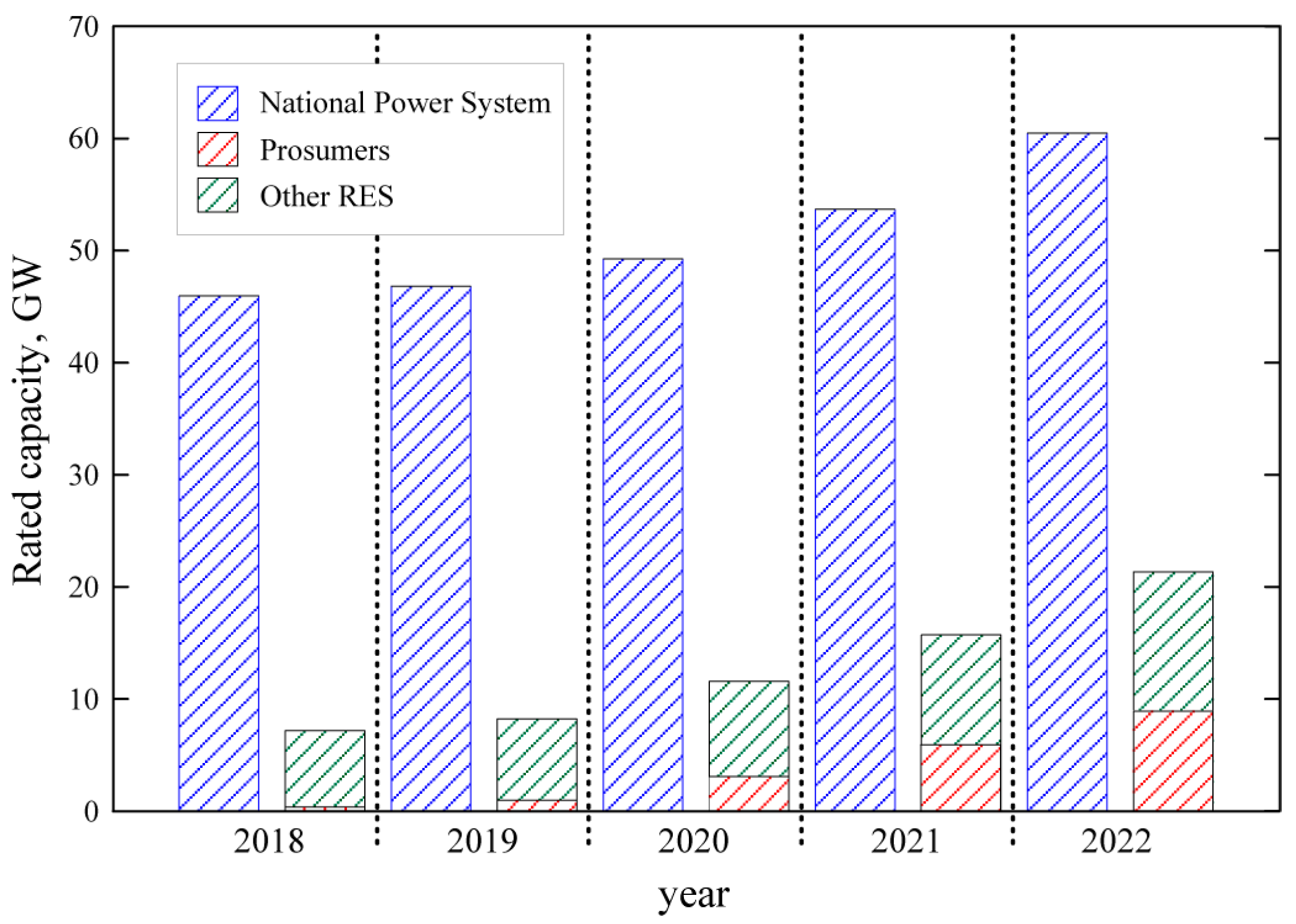Figure 1 shows the changes in the installed capacity of renewable energy source (RES)-based generator units over the last 5 years, compared to the total rated capacity of the generator units located in the National Electric Power System (NPS). As can be seen in Figure 1, the last 3–4 years have seen a sharp increase in the aggregate capacity of generation units—prosumer installations in particular.

In the European Union, solar energy plays a key role in the transition to clean energy and in the REPowerEU plan [3]. In 2023, according to SolarPower Europe, estimated solar generation capacity in the EU reached 259.99 GW, a significant increase from 164.19 GW in 2021 and 204.09 GW in 2022. This is part of a wider EU effort to increase the share of renewable energy and reduce dependence on imported fossil fuels and shows a change dynamic similar to that of Poland [4].

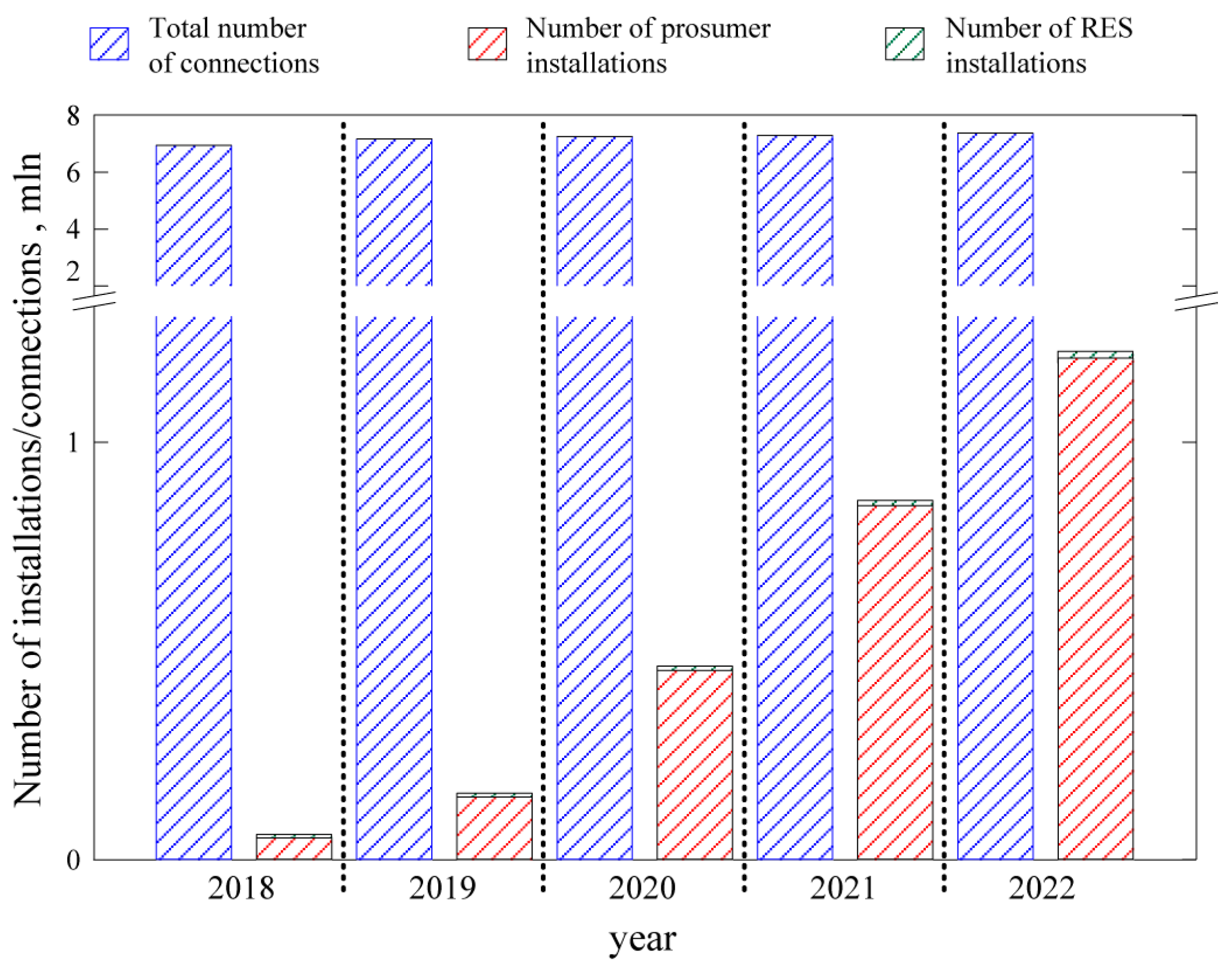
A prosumer installation should be understood as a node of the electricity grid, where we deal with both electricity consumption and generation [5]. Due to the nature of relatively easy connection of prosumer installations (on the so-called notification), they are mainly photovoltaic (PV) installations in low-voltage networks. These installations for distribution networks (low and medium voltage) are the same as RES-based installations, other renewable energy sources are of marginal importance. While the number of connections can be treated as almost constant (a change of 0.46 million (6.7%) connections over 5 years—from 6.7 million to 7.36 million), there is a very large change in the number of prosumer installations—at the end of 2022 year there were more than 1.2 million installations (a change of 1.15 million installations over 5 years—from 51 thousand to 1.2 million). Figure 2 shows the change in the number of RES installations (prosumer installations) in the distribution networks versus the total number of connections.

Figure 1. Changes in the rated capacity of generating units in the National Power System in the last 5 years [6,7].

Figure 1. Changes in the rated capacity of generating units in the National Power System in the last 5 years [6,7].

Figure 2. Changes in the number of prosumer installations (RES installations) compared to the total number of connections in distribution networks over the past 5 years [6].

Figure 2. Changes in the number of prosumer installations (RES installations) compared to the total number of connections in distribution networks over the past 5 years [6].

The dynamic growth of new prosumer installations poses a challenge not only to the operation of distribution networks, which must adapt, among other things, to the possibility of the emergence of two-way energy flow, but also on the operation of the entire power system. While in 2018–2019, for example, prosumer installations represented a margin in the total rated capacity of generating units, at the end of last year it was already about 15%, and when other RES-based installations are included, it is about 30%.

Many such distributed generation units in the power system, and in fact distribution networks, introduce quantitative as well as qualitative changes in their operation. These changes are observed primarily in the changes in power distributions. Quantitative changes in this case can be associated with lower demand for electricity of end users from the network (dependent, among other things, on self-consumption of energy at the place of generation or weather conditions), while qualitative changes are changes in the direction of power flow (cases of power flow from lower voltage networks to higher ones).

In scientific journals, one can find a growing number of analyses of the impact of PV installations on the operation of the distribution network—both medium and low voltage. The analyses carried out use various assumptions about generation and energy consumption. Considering a certain unpredictability of both the generation from PV microsources as well as the load profile of the grid during the day, a nondeterministic model approximating the real conditions of grid operation was developed using probabilistic tools [8].

A similar problem with the impact of a large numbers of prosumers with PV installations is noticed in the Slovak Republic, and the results of the study describe a stochastic methodology for PVHC estimation and use it to analyze a typical rural network of LV, presented in [9].

A different approach to analyzing the impact of PV installations on the operation of the distribution grid was taken in [10]. In this paper, results of analyses, based on the time-series method, are presented as risks for different levels of penetration of the photovoltaic sources, different divisions of the rated power of the photovoltaic sources between individual phases, and different consumer load profiles.

To solve the problem of excessively high voltage in a low-voltage distribution network with a large amount of distributed generation, a new approach to the use of electricity from these sources is proposed in [11]. To determine the advantages of the proposed solution, nine variants of the operation of an exemplary low voltage power grid over one day were analyzed using the electric multipole method and Newton’s method.

The other paper concerns the mitigation of voltage disturbances that deteriorate power quality and disrupt the operation of LV distribution grids due to the high penetration of PV energy sources in prosumer installations. The proposed solution is a novel control strategy for three-phase four-wire PV inverters, which ensures the transmission of active PV power and simultaneous compensation of load unbalance and reactive power, making the prosumer installation balanced and purely active [12].

Other solutions proposed in the literature for the problem under analysis are the use of energy storage for the control of the voltage level in the network [13].

This article shows the impact of solar photovoltaic installations on selected parameters of the operation of the low-voltage distribution network.

In the analyses presented here, three variants of generation and energy demand in relation to the connection capacity were assumed, considering the location of the substation feed analyzed section from the MFP. The variants considered focus on the ratio between generation and energy demand, which can correspond to the situation of extreme weather conditions—very bad or very good for generation. Variant two corresponds to balanced generation corresponding to demand. Such variants can occur due to both annual and daily variations.

For this purpose, the work is divided into four parts—introducing the issue, the essence of the distribution calculations, the results of the analyzed calculation example, and a summary of the analyzed issue.

2. Steady State Operation of the Power Grid

One of the effects of distributed generating units on the operation of the grid can be observed in steady-state conditions, in the values of such network operation parameters as voltage levels, branch current values, or power and energy losses. The network operation parameters mentioned above are determined based on the results of power flow calculations.

2.1. The Essence of Power Flow Calculations

Power flow calculations are concerned with determining the operating state of the power grid during the performance of its basic tasks—generation, transmission, and distribution of electricity, to ensure the continuous balancing of generated and received power. The primary purpose of such calculations is to determine the vector of nodal voltages (the so-called state vector), which is the basis for possible further analysis, i.e., determination of power flows, determination of power losses, or the issue of optimal voltage regulation.

Due to the specifics of the problem (a multidimensional system of nonlinear algebraic equations must be solved), the solution sought (the state vector) is determined based on iterative methods (such as the Gauss method or the Newton-Raphson method). In these methods, assuming an initial solution (usually it is the assumption that the levels of nodal voltages are equal to the nominal voltages of the network), a new solution is sought until the assumed criterion is met (usually it is the accuracy of changes in the obtained solution) [14].

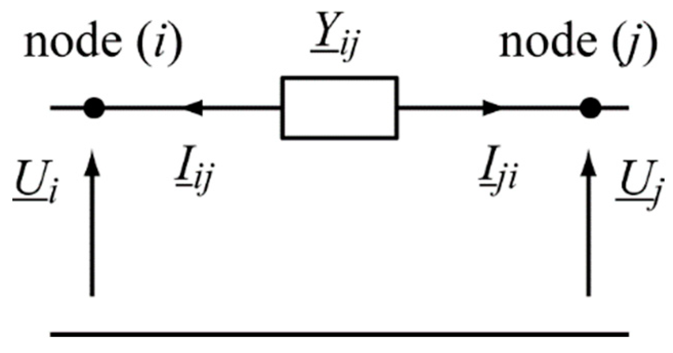
Based on the method of nodal potentials and the designations in Figure 3, the sought nodal voltage vector can be determined from the equation [14,15]:

$${\underset{\_}{U}}_i^{(k+1)}=\frac{1}{{\underset{\_}{Y}}_{ii}}\left(\frac{{\underset{\_}{S}}_i^{*}}{{\underset{\_}{U}}_i^{*\left(k\right)}}-\sum _{\begin{array}{c}j=1\\ j\ne i\end{array}}^w{\underset{\_}{Y}}_{ij}{\underset{\_}{U}}_j^{\left(k\right)}\right)$$

(1)

where: U_i, U_j is the voltage vector at a given node i, j, k is the iteration number, Y_ii is the intrinsic admittance of a given node i, Y_ij is the mutual admittance between nodes i and j, S_i is the apparent power consumed at a given node i, U_i^*, S_i^* is the conjugate of a complex number (voltage or apparent power).

2.2. Nodal Voltage Level

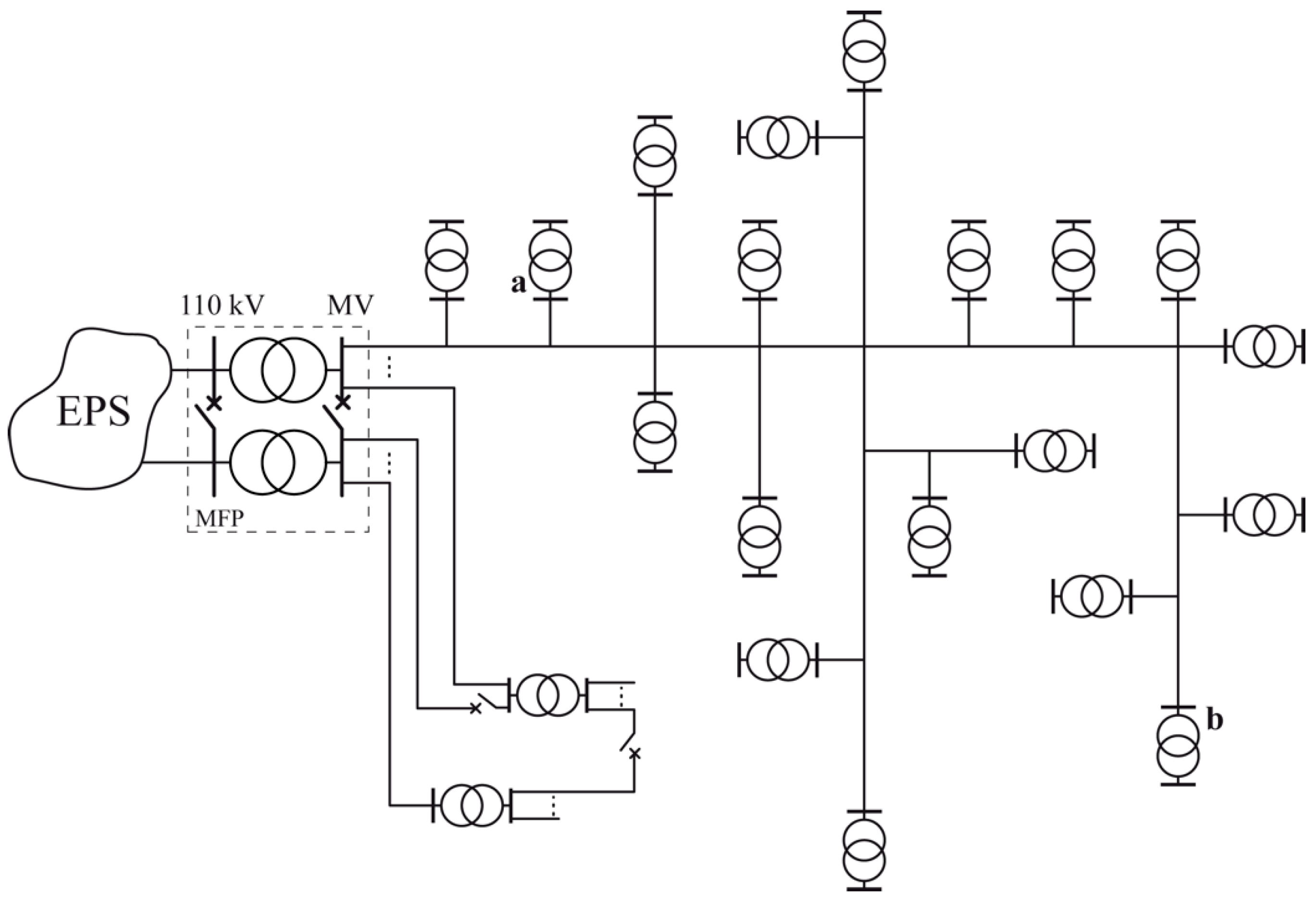
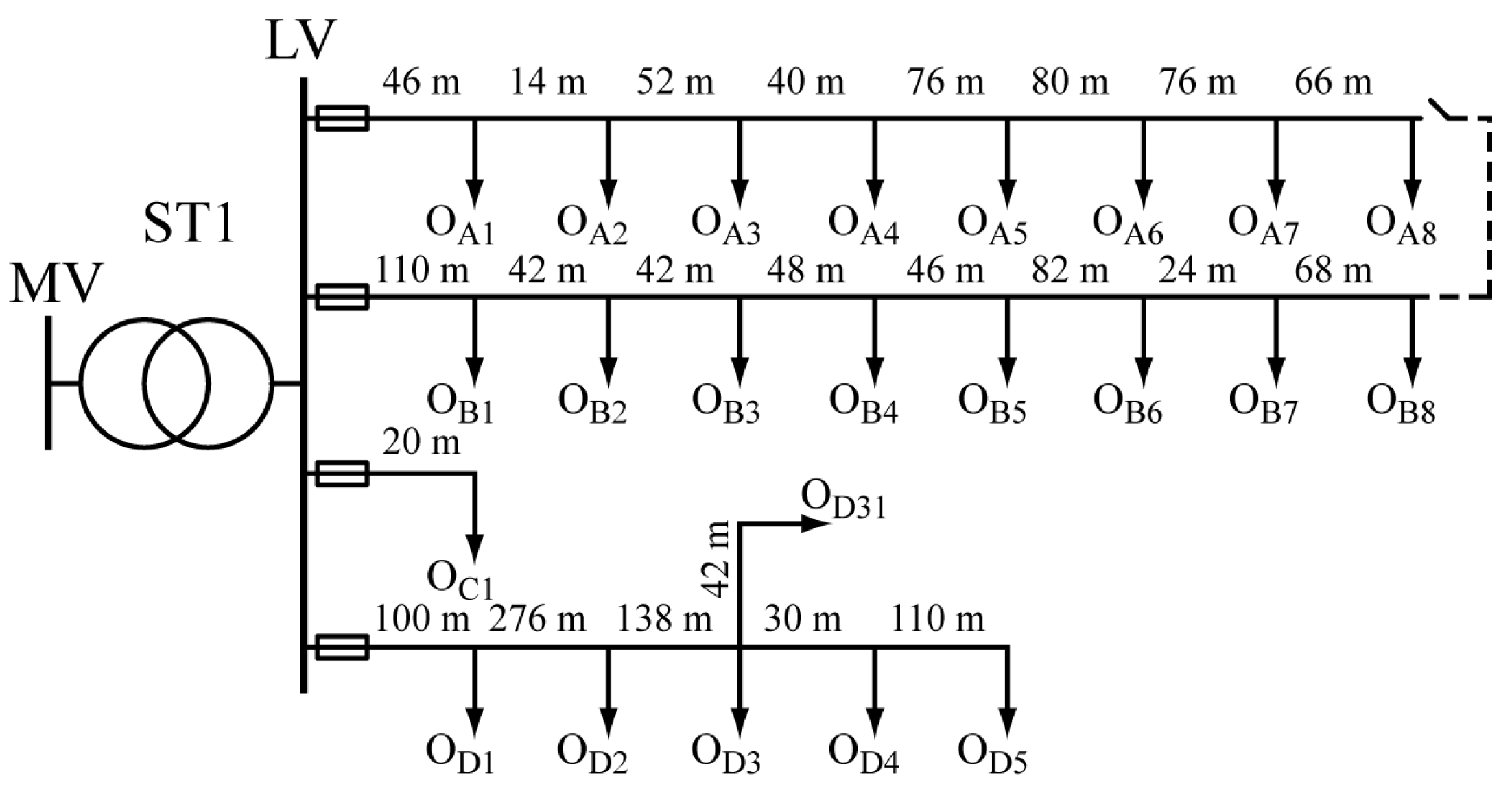
As shown in Figure 4, distribution networks are networks with open and closed structures, but operating in open configurations (open connectors at tie points). Regardless of the voltage level considered (MV or LV), for each node in the distribution network, the voltage deviation must be within the limits specified in the Decree of the Minister of Climate and Environment dated 22 March 2023 on detailed conditions for the operation of the electric power system, i.e., ±10% [16].

The expected level of voltage deviations at any node of the distribution network, fed by a given section of the 110 kV/MV substation, can be determined from the balance of voltage dips and deviations, according to the following equation:

• for the MV network: on MFP—ST1 station connection

  δU_MV% = δU_N − ∆U_MV

  (2)
• for the LV network: on MFP—consumer O_A8 connection

δU_LV% = δU_MV% + δU_θ + δU_PZ − ∆U_T − ∆U_LV

(3)

where: δU_MV%, δU_LV% is the voltage deviation in the MV and LV distribution network, δU_N is the voltage deviation from the nominal value of the network on the MV buses in the HV/MV substation, ∆U_MV is the voltage drop in the MV network, δU_θ is the voltage deviation associated with the difference between the ratio of the rated voltages of the MV/LV transformer and the ratio of the nominal voltages of the network, δU_PZ is the voltage deviation associated with the position of the on-load tap changer of the MV/LV transformer, ∆U_T is the voltage drop on the MV/LV transformer, ∆U_LV is the voltage drop on the LV network.

Equations (2) and (3) can be the basis, for example, of an analysis aimed at the optimal (from the point of view of the adopted criteria) regulation of voltage in the distribution network, having previously carried out distribution calculations—knowledge of branch currents/power is needed to calculate voltage drops on the various elements of the power network under consideration.

2.3. Branch Currents and Power Losses

The values of the currents flowing in each branch and the power flows can be determined based on the results of the flow calculations based on the following equations (for the designations shown in Figure 3):

I_ij = − (U_i − U_j)Y_ij = − I_ji

(4)

S_ij = − U_i(U_i^* − U_j^*)Y_ij^*

(5)

S_ji = − U_j(U_j^* − U_i^*)Y_ij^*

(6)

where: I_ij, I_ji is the current at the branch between node i and j, U_i, U_j is the voltage vector at a given node i and j, Y_ij is the mutual admittance between nodes i and j, S_ij, S_ji is the power at the branch between node i and j or j and i, U_i^*, U_j^*, Y_ij^* is the conjugate of a complex number.

Power losses in the branch between nodes i and j are the algebraic sum of the power flows determined from Equations (5) and (6).

3. The Analyzed Case of the Distribution Network Low Voltage

The analysis of the impact of the operation of the prosumers on selected parameters of the operation of the low voltage distribution network was carried out for the network with the structure shown in Figure 5, which is a development of the ST1 substation structure in Figure 4. The ST1 substation supplies four low voltage circuits, supplying a total of 23 consumers.

Calculations were made based on the following assumptions:

• the MV/LV substation has a transformer with the following parameters: S_N = 250 kVA, θ = 15.75/0.4 kV, ∆P_Cu = 3.25 kW, voltage short circuit u_sc% = 4.5%;
• the voltage conditions of the ST1 substation were determined based on Equations (2) and (3) and the assumed values of the parameters: δU_N = +5%, ∆U_LV = 1% or 10% (simulation of the location of the substation located near and far from the MFP—designation a and b in the analyzed variants of calculations), δU_θ = −5%, δU_PZ = +5%;
• the data of consumer nodes, i.e., max peak power P_max, power factor cosφ, connection power P_c and PV installation power P_PV are summarized in

  Table 1. Data of consumer nodes in the analyzed structure of the LV distribution network.

  Node	Pc [kW]	Pmax [kW]	cosφ	PPV [kW]
  A1	16	8.20	0.93	7
  A2	12	6.15	0.96	4
  A3	23	11.78	0.95	10
  A4	16	8.20	0.98	7
  A5	17	8.71	0.96	7
  A6	20	10.25	0.9	8.5
  A7	9	4.61	0.99	3
  A8	14	7.17	0.93	5.5
  B1	24	12.30	0.96	10
  B2	19	9.73	0.95	8.5
  B3	16	8.20	0.93	7
  B4	25	12.81	0.96	10
  B5	14	7.17	0.91	5.5
  B6	8	4.10	0.97	3
  B7	18	9.22	0.91	7
  B8	9	4.61	0.97	3
  C1	25	12.81	0.96	10
  D1	13	6.66	0.95	5.5
  D2	10	5.12	0.99	4
  D3	13	6.66	0.95	5.5
  D31	21	10.76	0.91	8.5
  D4	17	8.71	0.95	7
  D5	7	3.59	0.96	3

  ;
• the low-voltage line is made by the YAKY cable line, with three variants of the applied cross section of phase wires considered in the analyzes: 120 mm², 95 mm² and 70 mm². In the calculations, the following parameters were taken into account for the adopted cross sections: unit resistance R₀ equal to 0.253 Ω/km, 0.320 Ω/km and 0.443 Ω/km for the cross sections 120 mm², 95 mm² and 70 mm², respectively, and unit reactance X₀ equal to 0.1 Ω/km, regardless of the adopted cross section [17];
• the prosumer installations are of an older type, where the inverters operate in cosφ = 1 mode;
• calculations were made for three variants of the calculations considering the different degree of use of PV installations and the degree of demand in the analyzed grid structure. Variant 1 is the case where there are no PV installations, and we have 100% peak power demand. On the other hand, in Variant 2 and 3, we are dealing with a high number of PV installations, all consumers are prosumers, while the difference in the variants is in the degree of demand (Variant 2 and Variant 3 are peak power demand at 50% and 25%, respectively) and the degree of generation (Variant 2 and Variant 3 are generation at 50% and 100%).

4. Calculation Results and Discussion

In each calculation case, selected parameters of distribution network operation, i.e., voltage levels, branch current values, and power losses, were analyzed. Circuit A was analyzed in detail.

4.1. Nod’s Voltage Level

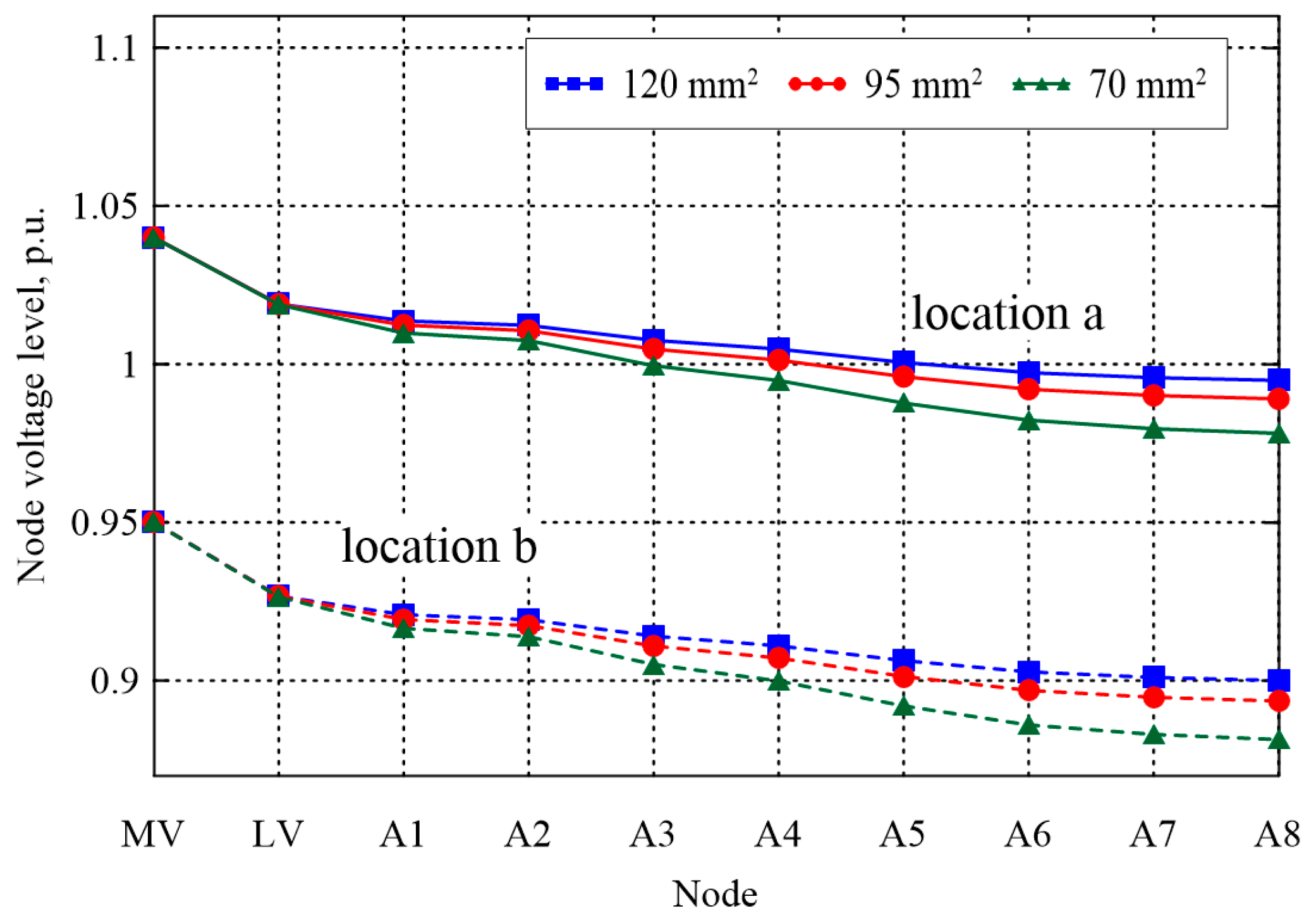
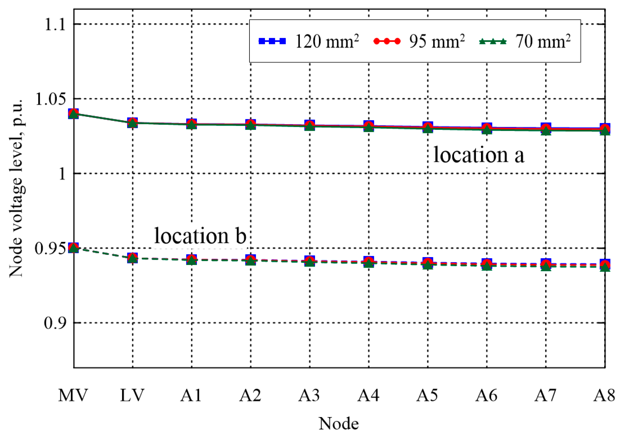
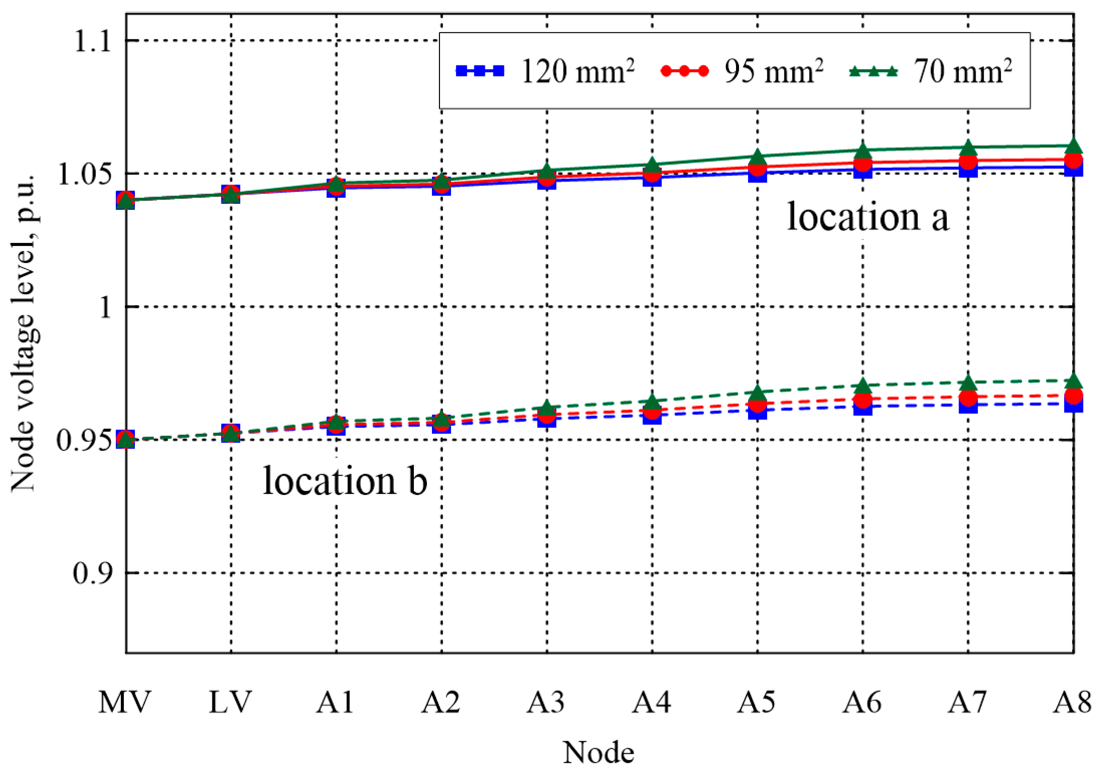
For the considered variants of the calculations, the distributions of voltage level changes along the path of the MV/LV transformer, consumer node in circuit A, are shown in Figure 6, Figure 7 and Figure 8.

For Variant 1 (without PV installation), regardless of the distance considered of the ST1 substation from the MFP (location a and location b), the situation of a decrease in the level of nodal voltage with an increase in the distance of the receiving node from the MV/LV transformer becomes apparent—qualitative changes in this case are similar. In turn, quantitative changes are to the detriment of location a, in which still for the network built with a cable line with a cross section of 120 mm², voltage levels are within the permitted limits of the regulation [16]; it is already for the cases of cross sections of 95 mm² and 70 mm² that we have exceedances of voltage deviations—from nodes A6 and A4, respectively.

For Variants 2 and 3 (simultaneous introduction of distributed generation and reduction of demand for electricity at consumer nodes), positively affect the changes in the voltage level in the analyzed network circuit for the adopted assumptions. For Variant 2, regardless of the cable line cross section used, we are dealing with a virtually constant voltage level in the network, equal to that of the MV/LV transformer. On the other hand, in Variant 3, the effect of the voltage increase is noticeable—the voltage level in the depth of the network is higher than in the supply node—the highest voltage increase was observed for the network built with a cable line with a cross section of 70 mm². For the adopted power supply conditions, the voltage levels obtained are within the allowed limits of the regulation [16]. Attention should be paid here to the situation of a possible change in the power supply conditions of MV/LV substations manifested, among other things, by a higher supply voltage (voltage regulation at the 110 kV/MV transformer or changes in the load level of the MV network). In such a situation (for Variant 3), the voltage boost shown may exceed the upper permissible voltage levels, resulting, among other things, in shutdowns of PV installations at prosumers.

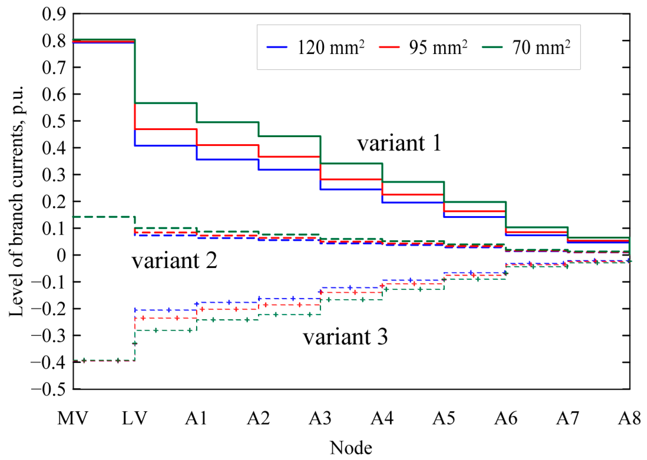
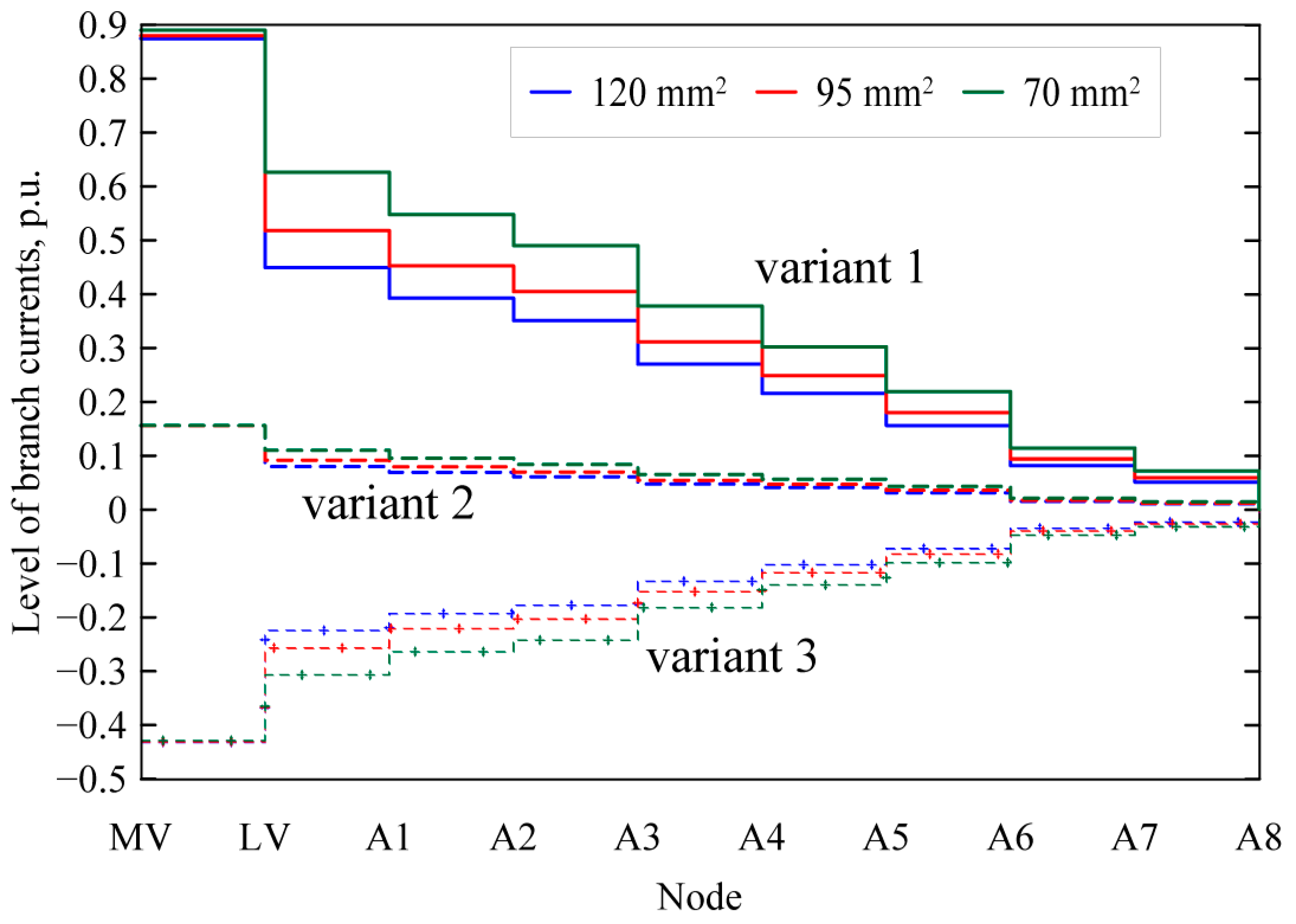
4.2. Values of Branch Currents

Quantitative and qualitative changes in the distribution of branch currents on the path of the MV/LV transformer—consumer node in circuit A, for the considered variants of calculations are shown in Figure 9 and Figure 10 for locations a and b, respectively. The changes shown are presented in relation to the values of the rated currents of the MV/LV transformer (applies only to branches between the MV and LV nodes) and the permissible current carrying capacities of cable lines for individual cross sections of phase conductors—based on [17], the values of Idop were assumed to be equal to 242 A, 211 A and 176 A, respectively, for cross sections of 120 mm², 95 mm² and 70 mm².

Regardless of the case of the location of the ST1 substation in relation to the 110 kV/SN substation (locations a and b shown in Figure 9 and Figure 10, respectively), identical trends of changes in the current values in individual branches were obtained from a qualitative point of view for Variants 1, 2, and 3. In the considered variants of calculations, we are dealing with a typical change in the values of currents in the analyzed network structure—the closer the supply node, the values of currents are increasingly higher, and the quantitative changes are related to the assumed conditions of electricity demand of consumer nodes. Moving from Variant 1 through Variant 2 to Variant 3, quantitative changes (the change in the degree of electricity demand of consumer nodes and the degree of generation in PV installations) become apparent, as well as qualitative changes manifested in the change in the direction of electricity flow. In Variant 1, it is a classic flow from the EPS to end users (energy flow in the right direction), in Variant 2, a very low degree of network loading can be observed (values close to zero, so that the level of node voltages is constant and close to the values of the supply of MV/LV substations), while in Variant 3, we are dealing with a flow opposite to the classic approach of supplying distribution networks (there is a flow of electricity from consumers to the EPS—in the left direction).

Regardless of the adopted power supply conditions and the degree of power demand of consumer nodes, a higher degree of current branch loading can also be observed in cases where the network is built on the smallest cross sections—in the case of the most heavily loaded branch (between nodes LV and A1), the observed relative changes are at the level of 15–20%.

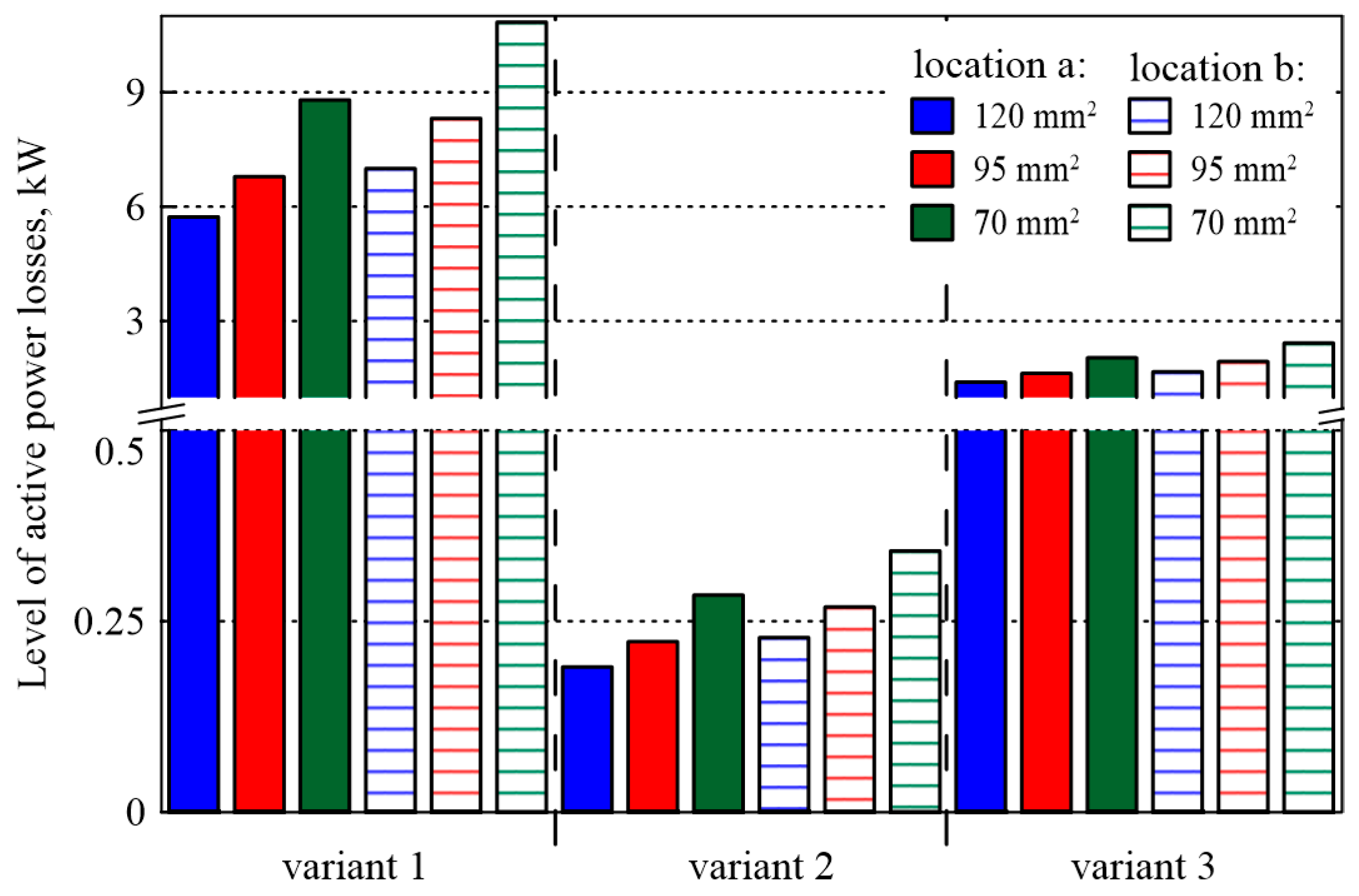
4.3. Level of Active Power Loss

Changes in the level of active power losses in the analyzed structure of the distribution network are shown in Figure 11. Regardless of the variant of calculations adopted related to the degree of electricity demand (Variants 1, 2, and 3) or the location of the ST1 substation in relation to the MFP (locations a and b), the highest loss values were obtained for the network built with a cable line with a cross section of 70 mm², and the lowest for a cable line with a cross section of 120 mm²—the influence of unit parameters in the creation of the equivalent scheme of the analyzed network.

The level of active power losses in the analyzed network is more influenced by the degree of electricity demand and the degree of electricity generation at individual consumer nodes. In the case of Variant 1 (the network only consumes electricity), there is more than a 50% increase in active power losses when changing from a cross section of 120 mm² to a cross section of 70 mm². Variant 2 represents an intermediate state between the qualitative changes in the distribution of current—the load of individual branches is very low, which translates into levels of active power losses (the multiplicity of value changes, relative to Variant 2, of the order of 30). For Variant 3, an increase in the level of power losses is again observed—despite the decrease in the degree of electricity demand, we are dealing here with an increased degree of electricity generation in prosumer installations. From the point of view of the operation of the analyzed network, there is a change in the direction of electricity flow with a simultaneous increase in the value of currents flowing in individual branches.

5. Conclusions

The article discusses the issue of the impact of the operation of prosumer installations on the operation of the low-voltage distribution network. The influence of prosumer installations can be observed, among other things, in the steady-state operation of the network. The article shows what influence prosumer installations can have on the values of such parameters of network operation as voltage level, values of branch currents and power losses. When analyzing selected parameters of distribution network operation, it should be remembered that their changes affect or are related to changes in other parameters. An example would be power supply conditions—the voltage level of the MV/LV substation. Expected lower values of nodal voltages, with constant power, are higher values of currents which in turn translates into a higher level of active power losses.

Three groups of assumptions were included in the analyzes, the simultaneous occurrence of which can pose a major problem for the correct operation of the low-voltage distribution network. These groups are: (1) a large number and power of prosumer installations in consumer nodes supplied from a given MV/LV substation (observed dynamic growth of prosumer installations in recent years); (2) a small degree of demand for electricity relative to the possibility of its generation (observed in the afternoon, during the hours with the greatest sunshine); (3) large values of parameter substitution schemes of the analyzed network structure (large values of unit resistance and reactance for networks with small cross sections).

The results shown from the analysis of the operation of prosumer installations on the operation of the distribution network can confirm the case of cooperation of prosumer installations with the low-voltage network without interference and without negative impact on its parameters and even their partial improvement. The shown influence of prosumer installations on the work of the distribution system has been limited to only one MV/LV substation—it should be remembered that there are many more such substations (supplied from the same outflow field in the MFP) and by improving the working conditions of one substation (the loads supplied from them), the working conditions of other substations can be worsened. The variants analyzed of the interaction of the PV installation with the grid showed that the effect depends both on the level of generation in relation to energy consumption and on the location of the line in question from the MFP substation.

According to Variant 2, the solution based on prosumer self-consumption is the most favorable for the grid. This solution assumes that the level of generation is close to the level of electricity demand with similar values of connection capacity and installed PV capacity. This solution is possible with an adjustment of the load profile and a change in prosumers’ approach to energy use. This change, for example, in rural areas can be based on the use of electricity to power greenhouses in agriculture based on crop growth mechanisms [18]. Similar conclusions are also presented in [11], where the advantages of changing the energy use profile of photovoltaic installations are demonstrated.

Detailed and reliable analyses of the operation of distribution networks should also be based on complete (covering the entire calendar year) profiles of electricity consumption of consumers, as well as profiles of electricity generation. Such issues constitute the next step of the analyses that the authors will undertake within the context of the issue at hand.