A Review on Economic Dispatch of Power System Considering Atmospheric Pollutant Emissions

Abstract

The environmental/economic dispatch (EED) of power systems addresses the environmental pollution problems caused by power generation at the operational level, offering macroscopic control without requiring additional construction and remediation costs, garnering widespread attention in recent years. This paper undertakes a comprehensive review of existing EED models, categorizing them according to the control of atmospheric pollutants into total air pollutant control (TAPC) and control considering the spatial and temporal diffusion (STD) of atmospheric pollutants. In addition, various methods employed to address the EED problems, as well as the current state of research on multi-area EED models, are presented. Finally, this paper analyzes and summarizes the literature on existing EED models, highlighting the deficiencies of the current work and future research directions. Through these explorations, the authors find that controlling the EED model by considering TAPC is more suitable for general macro planning, whereas the EED model considering the STD of air pollutant emissions enables more precise and effective control. Summarizing such models and techniques is conducive to developing dispatch plans adapted to local conditions, which is significantly beneficial for public welfare and government management, promoting sustainable and environmentally friendly power system dispatch methods.

1. Introduction

Environmental pollution has become a global issue, posing a severe threat to people’s lives. According to recent years’ data, only 10% of the assessed settlement populations were exposed to annual average levels of PM_2.5 or PM₁₀ that meet the World Health Organization’s air quality guidelines [1]. For NO₂, only 23% of the assessed settlement populations were exposed to annual average levels that meet the guidelines [2]. In recent years, in response to energy shortages, the reduction in air pollution, and the improvement of environmental quality, there has been a significant global increase in the proportion of renewable energy sources such as solar and wind power [3,4,5]. However, due to the natural conditions of primary energy sources, the coal-based power energy structure in some countries or regions will be difficult to change for a prolonged period in the future [6]. Therefore, addressing the environmental issues caused by the operation of coal-fired units is urgent. How to effectively reduce environmental pollution in the dispatch and operation of the power system has become one of the key issues in this research field [7,8].

The predominant atmospheric pollutants produced by coal-fired power generation units include particulate matter (PM), sulfur oxides (SO_x), and nitrogen oxides (NO_x), which are the main control subjects discussed in this paper. In recent years, scholars have extensively investigated strategies for developing low-air-pollution power systems, mainly including system planning methods [9,10,11], market regulation methods [12,13], policy guidance methods [14,15,16], and environmental–economic dispatch methods [17,18,19]. This paper provides a comprehensive review of relevant technical methods from the perspective of EED. The essence of the EED model focuses on the fundamental principle of “energy conservation and emission reduction”. Aligned with the operational and safety requirements of the system, it involves the optimal allocation of load among units to minimize total fuel costs and aggregate pollutant emissions within the dispatching cycle. This approach aims to substantially enhance the system operation’s economic and environmental facets while striving to curtail energy consumption and bolster environmental preservation to the greatest extent feasible. The EED model can be primarily categorized into two branches: the dispatching model considering TAPC and the dispatching model based on the optimization of the STD of air pollutant emissions. The former model has been subject to extensive research, and multiple countries have made various efforts to reduce their total emissions of air pollutants. However, there has been no significant improvement in the air quality of key residential environments in some local regions. This reflects the fact that the previous emission reduction measures were relatively crude. Existing power generation dispatch focuses on the centralized control of the system’s total emissions, insufficiently considering the intrinsic connections between population, energy, meteorology, and pollution. The latter model considers the STD of atmospheric pollutants, asserting that the concentration in the air determines the impacts of atmospheric pollutants on people’s lives and health. It is influenced by meteorological conditions, distance from pollutants, and other factors. There is relatively less existing research on the latter models, which require further exploration.

The EED problem typically exhibits high dimensionality, nonlinearity, and multiple constraints. Over the past few decades, various optimization methods have been applied to solve EED models. These methods can be broadly categorized into three types: (i) conventional methods, (ii) non-conventional methods, and (iii) hybrid methods. Conventional optimization methods are typically based on mathematical models and classical optimization theory. These methods are well established and widely understood, making them relatively easy to implement [20]. However, they may struggle to handle the complex constraints and nonlinearities often present in real-world power systems [21]. Non-conventional methods employ innovative artificial intelligence algorithms [22,23]. The advantage of non-conventional methods lies in their ability to work in a broader range of problem domains and their adaptability to complex, nonlinear problems. Nonetheless, they may require more computational resources and expertise to be implemented effectively. Hybrid methods combine the strengths of two or more algorithms, aiming to improve the convergence speed, handle large-scale problems, and integrate both theoretical and practical aspects to some extent [24].

Currently, there are several articles in the literature related to EED models. In 1994, Talaq J H et al. [25] conducted a comprehensive summary of the previous EED models, considering the types and controlled forms of environmental control variables. The discussions on the various models, however, lack sufficient detail. In 2018, Qu B Y et al. [26] and Fahad Parvez Mahdi et al. [27] successively published reviews on algorithms for solving EED problems; the former focused on summarizing algorithms for multi-objective optimization, while the latter provided a more comprehensive overview of the algorithms. Ismail Marouani et al. [28] presented an economic dispatch model that incorporates renewable energy sources like wind and solar power and revised the algorithms for addressing EED problems in 2022. Therefore, the existing literature reviews lack a detailed discussion on the STD model of air pollution, as well as a summary of its impact on dispatch models. This paper fills this gap. In terms of academic research, it provides researchers and readers with a comprehensive understanding of the classification and methodological frameworks of EED models, offering guidance to relevant scientific research personnel. In terms of application, the model methods introduced in this paper can provide technical personnel with macro technical guidance, facilitating their choice of appropriate implementation plans when considering different modeling and solution methods. At the same time, the improvement of EED technology enhances overall social welfare: it improves the health of residents, enables dispatchers to develop more efficient and environmentally friendly dispatch plans, and aids governments in achieving sustainable development and environmental protection goals.

The main contributions of this review paper are given as follows:

• Compared with previous reviews on the EED models, this paper further discusses the impact of coal-fired power units on atmospheric pollution: the models are divided into two categories, namely the EED model considering TAPC and the EED model based on the optimization of the STD of air pollutant emissions, and this paper introduces multi-area EED models, providing guidance for managing atmospheric pollution control models in regions.
• This paper provides a more detailed discussion and summary of the EED model based on the optimization of the STD of air pollutant emissions. It includes a comparison of the characteristics of the Gaussian plume model and the Gaussian puff model and a discussion of the influence of diurnal variations in the ABL. By considering the effects of the STD of air pollutants, flexible electricity dispatch decisions can be made in terms of economic and environmental impact, truly aiding in the sustainable development of the economy.
• Finally, this paper elaborates on the shortcomings of existing research on the EED models and explores future research directions. It is of great significance to further explore the flexibility resources of the power system to enhance environmental protection potential and adopt more advanced artificial intelligence algorithms for predicting atmospheric pollution and optimizing dispatch models.

The remainder of this paper is organized as follows: Section 2 and Section 3 introduce the EED model, considering TAPC and the EED model based on the optimization of the STD of air pollutant emissions, respectively. The solutions for solving EED problems are explained in Section 4. Section 5 discusses the multi-area EED model, and Section 6 presents the future directions of the EED model. Finally, the conclusion is given in Section 7.

2. The EED Model Considering TAPC

The earliest EED model can be traced back to 1971, when Gent M R and Lamont J W replaced the coal consumption minimization objective function in the static economic dispatch model with a system’s objective function aimed at minimizing NO_x emissions [29]. They included constraints for the NO_x emissions of individual units in the solution. Thus, the earliest EED model focused on a single-objective optimization dispatch problem for total atmospheric pollutant emissions. Subsequent environmental economic dispatch models have been extended and expanded within the framework summarized by Talaq J H [25].

The EED model considering TAPC typically refers to minimizing fuel costs and the total emissions of harmful gases and particulate matter while satisfying overall load demand and all other equations and inequality constraints. However, some researchers have also considered reliability levels, load adjustment times, reserve capacities, and even grid losses as additional objectives in the problem [30,31,32,33]. Generally, the problem can be formulated as follows [34,35,36]:

$$\min F(P_{\mathrm{G}})={\displaystyle \sum _{i=1}^{N_G}(a_i+b_i{P}_{\mathrm{G}i}+c_i{P}_{\mathrm{G}i}^2)}$$

(1)

where $a_i$, $b_i$, and $c_i$ are cost coefficients for the $i$-th coal-fired power generator. $F(P_{\mathrm{G}})$ is the total fuel cost of the system, while $N_{\mathrm{G}}$ identifies the number of coal-fired units. $P_{\mathrm{G}i}$ represents generator power for the $i$-th unit. If the fluctuation effects caused by the steam valve opening are taken into account, it requires adding sinusoidal components to the equation. Therefore, the cost function can be expressed as follows [37]:

$$\min F(P_{\mathrm{G}})={\displaystyle \sum _{i=1}^{N_G}(a_i+b_i{P}_{\mathrm{G}i}+c_i{P}_{\mathrm{G}i}^2+\left|d_i\sin [e_i(P_{\mathrm{G}i}^{\min }-P_{\mathrm{G}i})]\right|)}$$

(2)

where $d_i$ and $e_i$ are the cost coefficients of the $i$-th generator, while $P_{\mathrm{G}i}^{\min }$ is the minimum output of the $i$-th power generator.

When the coal is burned to generate power, it releases NO_x, SO_x, and PM. NO_x is created from the interaction between nitrogen and oxygen at high temperatures, while SO_x is formed by the combination of sulfur in coal with oxygen, resulting in the formation of sulfur dioxide. PM mainly consists of dust, smoke, and aerosols that are released during coal combustion [38,39]. These pollutants pose significant hazards to the atmospheric environment and human health. Various mathematical formulas have been developed to address this issue. It can be modeled using a quadratic function [25,40], a combination of a quadratic polynomial with an exponential term [41], or a combination of a quadratic equation with multiple exponential terms [28].

$$\min E(P_{\mathrm{G}})={\displaystyle \sum _{i=1}^{N_G}({\alpha }_i+{\beta }_i{P}_{\mathrm{G}i}+{\gamma }_i{P}_{\mathrm{G}i}^2)}$$

(3)

$$\min E(P_{\mathrm{G}})={\displaystyle \sum _{i=1}^{N_G}({\alpha }_i+{\beta }_i{P}_{\mathrm{G}i}+{\gamma }_i{P}_{\mathrm{G}i}^2+{\xi }_i\exp (\lambda \cdot P_{\mathrm{G}i}))}$$

(4)

$$\min E(P_{\mathrm{G}})={\displaystyle \sum _{i=1}^{N_G}({\alpha }_i+{\beta }_i{P}_{\mathrm{G}i}+{\gamma }_i{P}_{\mathrm{G}i}^2+{\xi }_{1i}\exp ({\lambda }_1\cdot P_{\mathrm{G}i})+{\xi }_{2i}\exp ({\lambda }_2\cdot P_{\mathrm{G}i}))}$$

(5)

where ${\alpha }_i$, ${\beta }_i$, ${\gamma }_i$, ${\xi }_i$, ${\xi }_{1i}$, ${\xi }_{2i}$, ${\lambda }_i$, ${\lambda }_{1i}$, and ${\lambda }_{2i}$ are the emission coefficients of the $i$-th power generator, and $E(P_{\mathrm{G}})$ is the total pollution emission of the system.

In the power system, numerous real-time and practical constraints play crucial roles in operation and planning. By effectively managing these constraints, the performance and stability of the power system can be significantly enhanced.

Table 1. The objectives and constraints commonly considered in the EED model.

Objectives	Constraints
Minimization of the total generation cost	Power balance constraint
Minimization of pollutant emissions	Generator limit constraint
Reliability level	Generators’ ramp rate limits
Load adjusting time	Power flow constraint
Reserve capacity	Prohibited operating zone constraints
Transmission loss	Emission constraints

illustrates some objectives and constraints that researchers consider to address the EED problem [27]. A description of some notable constraints is outlined below:

(1) Power balance constraint: The power balance constraint in an electric power system is a fundamental principle ensuring that the total electrical power generated matches the total power consumed within the system. It can be expressed as the following equation:

$${\displaystyle \sum _{i=1}^{N_{\mathrm{G}}}{P}_{\mathrm{G}i}=P_{\mathrm{D}}+P_{\mathrm{loss}}}$$

(6)

where $P_{\mathrm{D}}$ and $P_{\mathrm{loss}}$ stand for total power demand and total loss, respectively.

(2) Generator limit constraint: The generator limit constraint in a power system refers to the limitations imposed on each generator’s output capacity. This constraint is expressed as an inequality for each generator $i$ in the system:

$$P_{\mathrm{G}i}^{\min }\le P_{\mathrm{G}i}\le P_{\mathrm{G}i}^{\max }$$

(7)

where $P_{\mathrm{G}i}^{\max }$ is the maximum output of the $i$-th power generator.

(3) Generators’ ramp rate limits: This constraint ensures that the rate of change in power output remains within the specified limits for each generator. It can be expressed as follows:

$$\max (P_{\mathrm{G}i}^{\min },P_{\mathrm{G}i}^0-D{R}_i)\le P_{\mathrm{G}i}\le \min (P_{\mathrm{G}i}^{\max },P_{\mathrm{G}i}^0+U{R}_i)$$

(8)

where $P_{\mathrm{G}i}^0$ refers to the previous operating point of the $i$-th power generator, and $D{R}_i$ and $U{R}_i$ are the downward rate limit and upward rate limit of the $i$-th power generator, respectively.

(4) Power flow constraint: Transmission lines in the power system are responsible for transmitting electrical energy generated by power generators to various loads. However, due to the finite capacity of these lines, constraints on power flow are necessary to avoid exceeding the line’s carrying capacity, prevent overloading, and ensure the stability and reliability of the system. It can be described as follows:

$$\left|S_{li}\right|\le S_{li}^{\max },i=1,2,\dots N_{\mathrm{L}}$$

(9)

where $S_{li}$ and $S_{li}^{\max }$ are the transmission line loading and the maximum transmission line loading, respectively, while $N_{\mathrm{L}}$ is the number of transmission lines.

(5) Prohibited operating zone constraints: In actual power generation systems, the entire operating range of generating units is not always available for operation. Operations within these zones may lead to system instability, equipment damage, or other adverse consequences. Therefore, power generation output must avoid operating in prohibited operating zones. Generator unit $i$ should operate within the feasible operating zones, as described below [27]:

$$P_{\mathrm{G}i}=\left\{\begin{array}{l}{P}_{\mathrm{G}i}^{\min }\le P_{\mathrm{G}i}\le P_{\mathrm{G}i,1}^L,\hfill \\ P_{\mathrm{G}i,j-1}^U\le P_{\mathrm{G}i}\le P_{\mathrm{G}i,j}^L,j=2,3\dots ,K_i\hfill \\ P_{\mathrm{G}i,K_i}^U\le P_{\mathrm{G}i}\le P_{\mathrm{G}i}^{\max },\hfill \end{array}\right.$$

(10)

where $K_i$ represents the number of prohibited operation zones in the curve of the $i$-th power generator, while $j$ represents the index of the prohibited operating zone of the $i$-th power generator. $P_{\mathrm{G}i,j}^L$ and $P_{\mathrm{G}i,j-1}^U$ represent the lower limit of the $j$-th prohibited operating region and the upper limit of the $(j-1)$-th prohibited operating region for the $i$-th power generator.

(6) Emission constraints: Emission constraints typically involve key pollutants such as SO_x, NO_x, and PM. These constraints are designed to minimize adverse environmental impacts and ensure that human activities have a manageable influence on the atmosphere, water bodies, and soil [42,43].

$$E_{\mathrm{S}}\le L_{{\mathrm{SO}}_{\mathrm{x}}},E_{\mathrm{N}}\le L_{{\mathrm{NO}}_{\mathrm{x}}},E_{\mathrm{PM}}\le L_{\mathrm{PM}}$$

(11)

where $E_{\mathrm{S}}$, $E_{\mathrm{N}}$, and $E_{\mathrm{PM}}$ are the gases’ emissions, respectively, of NO_x, SO_x, and PM. $L_{{\mathrm{SO}}_{\mathrm{x}}}$, $L_{{\mathrm{NO}}_{\mathrm{x}}}$, and $L_{\mathrm{PM}}$ are the maximum limits of emissions of different gases.

3. The EED Model Based on the Optimization of the STD of Air Pollutant Emissions

As mentioned in the previous section, most current EED models are based on controlling the total emissions of atmospheric pollutants within the studied area. However, the ground-level pollutant concentration (GLPC) is the primary assessment index directly affecting human health and causing economic losses. The GPLC is related to factors such as the emissions conditions (e.g., emission volume, emission height, emission method, and dispersion patterns of the emissions), meteorological conditions, and topographical features. Therefore, it is necessary to delineate the relationship between emissions from coal-fired power plants and the resultant ground-level concentrations, aiming to initiate environmental–economic optimization dispatch from the perspective of reducing GPLC.

3.1. Basic Framework for the STD Calculation of Atmospheric Pollutants

Establishing the source–receptor mapping relationship between pollutant emissions from coal-fired units and regional pollutant concentrations requires the utilization of gas dispersion models. The gas dispersion models are mathematical models used to simulate and predict the STD, as well as for the propagation patterns of pollutants in the atmosphere. These models typically integrate knowledge from various fields, such as atmospheric dynamics, meteorology, chemical kinetics, and geographic information systems, to provide a quantitative description of the dispersion behavior of atmospheric pollutants. Simultaneously, power dispatch itself presents a nonlinear problem with multiple variables and constraints. Therefore, to accurately and rapidly assess the diffusion of pollutants from these coal-fired units, the model meets the following conditions: (1) It takes into account the impact of the ABL, fully reflecting the diffusion characteristics of pollutants from elevated point sources such as power plants; (2) It considers the types of pollutants emitted by coal-fired power plants, including PM, SO_x, NO_x, etc.; (3) It requires low parameters and is easy to calculate; (4) It has a wide range of applicability and can be used for the environmental conditions of most coal-fired units. The Gaussian dispersion model serves as the physical foundation for many practical dispersion models, featuring the advantages of simple expression, convenient computation, and compatibility with other issues. In the short-term dispatching optimization problems of the power system, the diffusion of pollutants emitted from coal-fired power plants in the atmosphere is mainly influenced by primary characteristics, with the indirect effects from secondary or multiple physical and chemical reactions not yet manifested. Therefore, the Gaussian dispersion model can be employed to describe the dispersion process of pollutants emitted during power production in the atmosphere. The Gaussian dispersion model includes the Gaussian plume model and the Gaussian puff model, which will be elaborated below.

3.1.1. Gaussian Plume Model

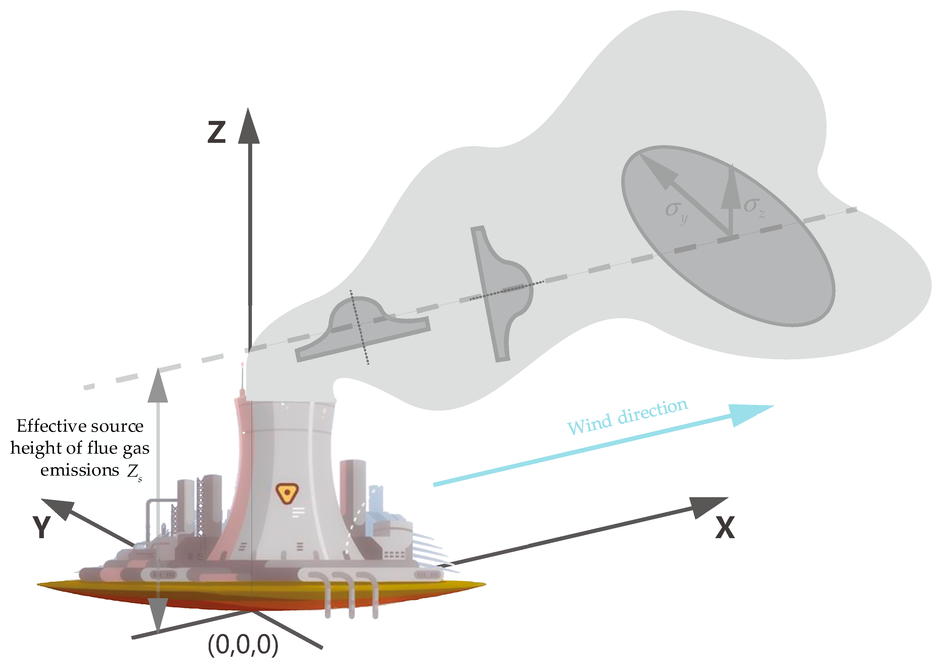
The Gaussian plume model is a mathematical model used to estimate the distribution of pollutant concentrations in the atmosphere. Based on Gaussian distribution, the model simulates the dispersion of air pollutants in the atmosphere in the form of a Gaussian curve. The model assumes stable atmospheric conditions near the emission source, exhibiting Gaussian distribution in both horizontal and vertical directions. It utilizes wind field information and dispersion parameters to describe the pollutant dispersion process in the atmosphere, establishing a three-dimensional coordinate system with the wind direction as the $x$-axis and the ground at the chimney’s location as the coordinate origin, as shown in Figure 1 [44].

Under the assumption of constant horizontal wind speed $\overline{u}$, the pollutants spread at the same rate in a direction perpendicular to the wind. The air quantity passing through the plume flow section per unit time can be represented by $\overline{u}\pi r^2$, where $r$ represents the cross-sectional radius. The total flux of pollutants on any vertical plane downstream of the pollution source should be equal to the total mass emitted in unit time. It can be expressed as follows [45]:

$${\displaystyle \int {\displaystyle \underset{-\infty }{\overset{+\infty }{\int }}\overline{u}}}{C}_{\mathrm{GLPC}}\left(x,y,z\right)dydz=\sum _{i=1}^{N_{\mathrm{G}}}{E}_{\tau }(P_{\mathrm{G}i})$$

(12)

where $C_{\mathrm{GLPC}}\left(x,y,z\right)$ represents the GLPC at a certain geographical location. $\tau$ represents the time of the pollutant emission, while $E_{\tau }(P_{\mathrm{G}i})$ stands for the mass of the $i$-th power generator emitting the plume at time $\tau$.

The GLPC at the location $(x,y,z)$ can be expressed as follows:

$$C_{\mathrm{GLPC}}\left(x,y,z\right)=\frac{{\displaystyle \sum _{i=1}^{N_{\mathrm{G}}}}{E}_{\tau }(P_{\mathrm{G}i})}{\overline{u}\pi r^2}$$

(13)

However, pollutants do not exhibit a uniform distribution in horizontal and vertical diffusion perpendicular to the wind direction. In the Gaussian plume model, the diffusion of atmospheric pollutants can be considered to flow firstly in the direction of the wind and then to spread outwards, with the distribution of pollutant concentration conforming to a Gaussian distribution, as shown in Figure 1. ${\sigma }_y$ and ${\sigma }_z$ represent the variances in pollutant dispersion in the horizontal and vertical directions, respectively, as horizontal and vertical diffusion parameters. These parameters characterize the diffusion range of pollutants in the $y$ and $z$ directions.

Therefore, according to the expression of the Gaussian distribution, the Gaussian plume dispersion model for elevated continuous point sources can be represented as

$$C_{\mathrm{GLPC}}\left(x,y,z\right)=A(x)e^{-a{y}^2}{e}^{-b{z}^2}$$

(14)

${\sigma }_y$ and ${\sigma }_z$ can be derived through probability statistical theory.

$$\left\{\begin{array}{c}{\sigma }_y^2=\frac{{\displaystyle {\int }_0^{\infty }{y}^2{C}_{\mathrm{GLPC}}dy}}{{\displaystyle {\int }_0^{\infty }{C}_{\mathrm{GLPC}}dy}}\\ {\sigma }_z^2=\frac{{\displaystyle {\int }_0^{\infty }{z}^2{C}_{\mathrm{GLPC}}dz}}{{\displaystyle {\int }_0^{\infty }{C}_{\mathrm{GLPC}}dz}}\end{array}\right.$$

(15)

We substituted Equation (14) into Equation (15) and integrated to obtain

$$\left\{\begin{array}{c}a=\frac{1}{2{\sigma }_y^2}\\ b=\frac{1}{2{\sigma }_z^2}\end{array}\right.$$

(16)

We substituted Equations (14) and (16) into Equation (12) and performed the integration, resulting in

$$A(x)=\frac{{\displaystyle \sum _{i=1}^{N_{\mathrm{G}}}}{E}_{\tau }(P_{\mathrm{G}i})}{2\overline{u}\pi {\sigma }_y{\sigma }_z}$$

(17)

After substituting Equations (16) and (17) back into Equation (14) and considering the effects of dynamic lift and coal-fired lift, the concentration distribution function of the pollutants emitted from the power plant could be expressed as

$$C_{\mathrm{GLPC}}\left(x,y,z\right)=\frac{{\displaystyle \sum _{i=1}^{N_{\mathrm{G}}}}{E}_{\tau }(P_{\mathrm{G}i})}{2\overline{u}\pi {\sigma }_y{\sigma }_z}\exp [-\frac{1}{2}\left(\frac{y^2}{{\sigma }_y^2}+\left(\frac{z-{Z_s}^2}{{\sigma }_z^2}\right)\right)]$$

(18)

where $Z_s$ represents the effective source height of flue gas emissions. In practical engineering, monitoring points are set at ground level, taking $z=0$, so Equation (18) is reformulated as

$$C_{\mathrm{GLPC}}\left(x,y,z\right)=\frac{{\displaystyle \sum _{i=1}^{N_{\mathrm{G}}}}{E}_{\tau }(P_{\mathrm{G}i})}{2\overline{u}\pi {\sigma }_y{\sigma }_z}\exp [-\frac{1}{2}\left(\frac{y^2}{{\sigma }_y^2}+\frac{{Z_s}^2}{{\sigma }_z^2}\right)]$$

(19)

In the atmospheric process of pollutant transport and diffusion, various removal and transformation mechanisms act collectively. These mechanisms result in the reduction in and alteration of pollutants in the air, thereby influencing the concentration distribution and spatiotemporal variations in the atmosphere. The typical approach is to assume an exponential decay of pollutant mass over time. Therefore, the GLPC caused by pollutants emitted at time $\tau$ at location $(x,y)$ during monitoring time $t$ can be expressed as [45]

$$C_{\mathrm{GLPC}}\left(\tau ,t^{\text{'}};x,y\right)=\frac{{\displaystyle \sum _{i=1}^{N_{\mathrm{G}}}}{E}_{\tau }(P_{\mathrm{G}i})}{2\overline{u}\pi {\sigma }_y{\sigma }_z}\exp (-\frac{t^{\text{'}}-\tau }{T_{res}})\exp [-\frac{1}{2}\left(\frac{y^2}{{\sigma }_y^2}+\frac{{Z_s}^2}{{\sigma }_z^2}\right)]$$

(20)

where $t^{\text{'}}$ denotes the monitoring time of air quality. $T_{res}$ represents the residence time of the pollutant puff, signifying the average lifespan of atmospheric pollutants during continuous physical–chemical decay. It is generally considered that after a duration $T_{res}$ from the emission time $\tau$ of the plume, the impact of the pollutant plume on the concentration level of atmospheric pollution is negligibly small.

From the above discussion, the characteristics of the Gaussian plume model are as follows:

• The model typically assumes that the environmental conditions of the atmosphere and emission sources remain in a steady state during the simulated time period.
• This makes the model suitable for short-term predictions. In the direction of wind flow, when the wind speed is greater than the dispersion speed, advective transport has a much greater impact than diffusion.
• The model may fail in complex atmospheric environments, for example, under conditions of an unstable atmosphere or non-uniform wind fields.

In reality, meteorological conditions such as wind speed will continuously change with the movement of pollutants and the passage of time. If the Gaussian plume model is used to estimate the GLPC from power plants, it will fail to reflect the impacts of changing meteorological conditions and emission rates. Therefore, the Gaussian plume model is not suitable for actual power dispatch scenarios with variable meteorological conditions and continuously changing power plant output [45].

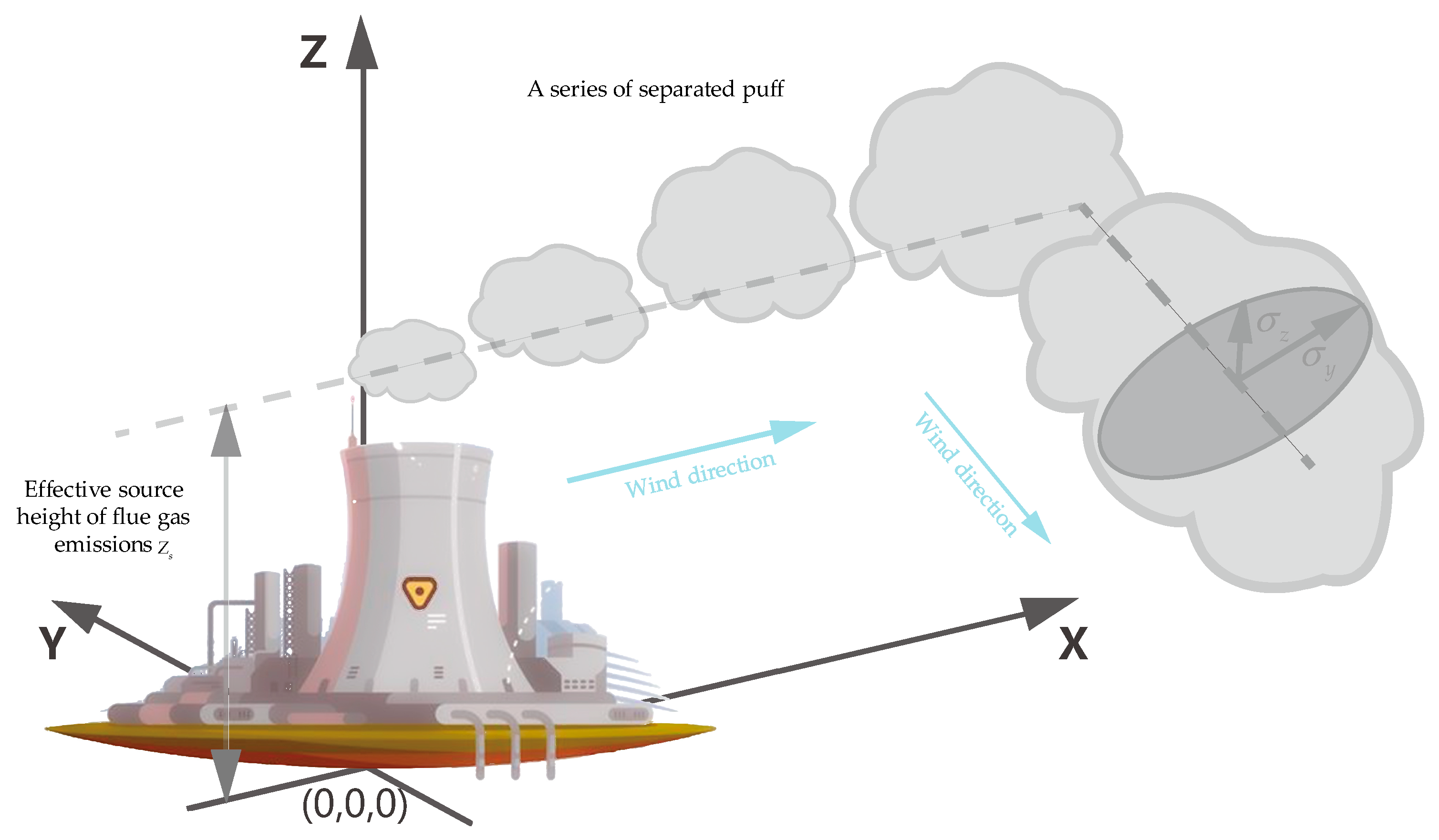
3.1.2. Gaussian Puff Model

The Gaussian puff model treats instantaneous pollutant emissions as a puff, as illustrated in Figure 2 [46,47]. As the puff moves with the wind, it undergoes diffusion by expanding its diameter. In comparison to the traditional Gaussian plume model, the Gaussian puff model is more suitable for describing situations with rapid changes in wind speed and wind direction over short periods. It is commonly employed for short-term air quality simulations. Clearly, the time difference $\Delta t_{puff}$ between two adjacent puffs should be sufficiently small to ensure the accuracy of simulations of the original continuous plume. Typically, the basic time step $\Delta t_{puff}$ for puff emissions should satisfy the following equation [48]:

$${[u^2+v^2]}^{1/2}\Delta t_{puff}\le R_{py}$$

(21)

where $u$ and $v$ are the wind speeds in the $x$ and $y$ directions at any given moment, respectively. $R_{py}$ represents the half-width of the puff, typically set as ${\sigma }_x={\sigma }_y$ and defined as $R_{py}=2.15{\sigma }_y$.

The Gaussian puff model also assumes that the dispersion of pollutants in both horizontal and vertical directions follows a Gaussian distribution. It further assumes that the emission intensity, wind speed, wind direction, and atmospheric stability are constant during the basic time step. The GLPC at the location $(x,y,z)$ can be expressed as follows [49]:

$$C_{\mathrm{GLPC}}\left(\tau ,t^{\prime };x,y,z\right)=\sum _{i=1}^{N_{\mathrm{G}}}\sum _{\tau =t^{\prime }-T_{res}}^{t^{\prime }-1}{E}_{\tau }(P_{\mathrm{G}i})G_i\left(\tau ,t^{\prime };x,y,z\right)\cdot \exp \left(-\frac{t^{\prime }-\tau }{T_{res}}\right)$$

(22)

In Equation (22), $G_i(\cdot )$ represents the dispersion distribution function of puff emitted from the pollution source, expressed as

$$\begin{array}{c}{G}_i\left(\tau ,t^{\prime };x,y,z\right)={\left({(2\pi )}^{\frac{3}{2}}{\sigma }_x\left(\tau ,t^{\prime }\right){\sigma }_y\left(\tau ,t^{\prime }\right){\sigma }_z\left(\tau ,t^{\prime }\right)\right)}^{-1}\cdot \\ \exp \left(-\frac{1}{2}\left({\left(\frac{x-x_{\mathrm{c}}\left(\tau ,t^{\prime }\right)}{{\sigma }_x\left(\tau ,t^{\prime }\right)}\right)}^2+{\left(\frac{y-y_{\mathrm{c}}\left(\tau ,t^{\prime }\right)}{{\sigma }_y\left(\tau ,t^{\prime }\right)}\right)}^2+{\left(\frac{z-z_{\mathrm{c}}\left(\tau ,t^{\prime }\right)}{{\sigma }_z\left(\tau ,t^{\prime }\right)}\right)}^2\right)\right)\end{array}$$

(23)

where ${\sigma }_x\left(\tau ,t^{\prime }\right)$, ${\sigma }_y\left(\tau ,t^{\prime }\right)$ and ${\sigma }_z\left(\tau ,t^{\prime }\right)$ represent the diffusion parameters in the three dimensions $x$, $y$, and $z$ respectively, while $x_{\mathrm{c}}\left(\tau ,t^{\prime }\right)$, $x_y\left(\tau ,t^{\prime }\right)$, and $x_z\left(\tau ,t^{\prime }\right)$ denote the coordinates of the puff center. These coordinates continuously update at different monitoring times [50,51].

$$\left[\begin{array}{l}{x}_{\mathrm{c}}\left(\tau ,t^{\prime }\right)\hfill \\ y_{\mathrm{c}}\left(\tau ,t^{\prime }\right)\hfill \\ z_{\mathrm{c}}\left(\tau ,t^{\prime }\right)\hfill \end{array}\right]=\left[\begin{array}{l}{x}_{\mathrm{s}}\hfill \\ y_{\mathrm{s}}\hfill \\ z_{\mathrm{s}}\hfill \end{array}\right]+\sum _{t=\tau +1}^{t^{\prime }}\left[\begin{array}{c}u(t)\\ v(t)\\ w(t)\end{array}\right]\mathsf{\Delta }t$$

(24)

where $x_s$, $y_s$, and $z_s$ represent the three-dimensional geographical coordinates of the coal-fired power plant’s pollution source; $t$ signifies a particular moment between the puff emission time and the monitoring point’s observation time; $\mathsf{\Delta }t$ denotes the time interval between the two observation times, often set as $\mathsf{\Delta }t=1\mathrm{h}$; and $u(t)$, $v(t)$, and $w(t)$, respectively, indicate the average wind speeds in the $x$, $y$, and $z$ directions over the time interval $\mathsf{\Delta }t$.

When the atmospheric environment remains stable within the time interval $[\tau ,t]$, the diffusion parameters from moments $\tau$ to $t$ satisfy

$$\left\{\begin{array}{l}{\sigma }_x(\tau ,t)={\sigma }_y(\tau ,t)=\alpha (t){(t-\tau )}^{\lambda (t)}\hfill \\ {\sigma }_z(\tau ,t)=\beta (t){(t-\tau )}^{\gamma (t)}\hfill \end{array}\right.$$

(25)

where $\alpha$, $\beta$, $\lambda$, and $\gamma$ represent the calculation coefficients for the diffusion parameters, contingent upon the atmospheric stability grade of the puff center at various moments.

According to GB/T 3840-91 [52], atmospheric stability is categorized into six levels: very unstable, unstable, weakly unstable, neutral, moderately stable, and stable, where a lower stability level indicates higher atmospheric instability. These are denoted by the letters A, B, C, D, E, and F, respectively [53]. The coefficients for Equation (25), as summarized by the Japanese Ministry of the Environment [54], are presented in the

Table 2. The horizontal diffusion parameter calculation coefficients.

Atmospheric Stability Level	$\mathit{\alpha }$	$\mathit{\lambda }$
A	1.92091	0.88479
B	1.42501	0.89034
C	1.01538	0.89635
D	0.68240	0.88671
E, F	0.61003	0.88547

and

Table 3. The vertical diffusion parameter calculation coefficients.

Atmospheric Stability Level	$\mathit{\beta }$	$\mathit{\gamma }$	$\mathit{t} - \mathit{\tau }/\mathit{s}$
A	0.22821	1.16593	0~500
	0.04906	1.41327	500~2000
	0.01726	1.55074	2000~$\infty$
B	0.36076	1.01128	0~1000
	0.19202	1.11026	1000~$\infty$
C	0.42641	0.91251	0~$\infty$
D	0.44691	0.85576	0~1000
	1.30023	0.70115	1000~$\infty$
E	0.52328	0.77422	0~1000
	1.40800	0.63093	1000~3000
	4.09832	0.49749	3000~$\infty$
F	0.64000	0.69897	0~1000
	1.02400	0.63003	1000~3000
	4.65031	0.44197	3000~$\infty$

.

Taking the standards for atmospheric pollutant emissions in China as an example, determining atmospheric stability involves several calculation and analysis steps [55].

Firstly, the calculation of the solar declination angle $\delta$ is performed using the following formula:

$$\begin{array}{c}\delta =(0.006918-0.399912\cos {\theta }_0+0.070257\sin {\theta }_0-0.006758\cos 2{\theta }_0\\ +0.000907\sin 2{\theta }_0-0.002697\cos 3{\theta }_0+0.001480\sin 3{\theta }_0)\cdot \frac{180}{\pi }\end{array}$$

(26)

$${\theta }_0=\frac{360d_n}{365}$$

(27)

where $d_n$ represents the ordinal date within a year, with values in the range 0, 1, 2, …, 364, indicating the chronological order of the day within the year.

Secondly, we introduce the solar declination angle $\delta$ as a computational parameter, and the calculation of the solar radiation angle $h_0$ is obtained using the following formula:

$$h_0=\arcsin (\sin \varphi \sin \delta +\cos \varphi \cos (15t+\lambda -300))$$

(28)

where $\varphi$ represents the local geographical latitude, and $\lambda$ represents the local geographical longitude. Given the variability in geographical coordinates, the solar radiation angle differs accordingly. Following the computation of the solar elevation angle for a specific day, the corresponding solar radiation level for that day can be determined by referencing

Table 4. Solar radiation level according to cloud condition and solar radiation.

Total Cloud Cover/Low Cloud Cover	Night Time	Solar Radiation Angle
		${\mathit{h}}_0\le 15^{°}$	$15^{°}<{\mathit{h}}_0\le 35^{°}$	$35^{°}<{\mathit{h}}_0\le 65^{°}$	${\mathit{h}}_0>65^{°}$
$\le 4/\le 4$	−2	−1	+1	+2	+3
$5~7/\le 4$	−1	0	+1	+2	+3
$\ge 8/\le 4$	−1	0	0	+1	+1
$\ge 5/5~7$	0	0	0	0	+1
$\ge 8/\ge 8$	0	0	0	0	0

based on the observed cloud-cover conditions [56].

Finally, the atmospheric stability level is obtained in

Table 5. Atmospheric stability level according to solar radiation and ground-level wind speed.

Ground-Level Wind Speed (m/s)	Solar Radiation Level
	+3	+2	+1	0	−1	−2
$\le 1.9$	A	A~B	B	D	E	F
$2~2.9$	A~B	B	C	D	E	F
$3~4.9$	B	B~C	C	D	D	E
$5~5.9$	C	C~D	D	D	D	D
$\ge 6$	D	D	D	D	D	D

[56].

If the atmospheric stability remains constant from moment $\tau$ to $t$ and there is a change in atmospheric stability at time $t+\Delta t$, then the atmospheric diffusion parameters follow a continuous transitional relationship [50,57] as follows:

$$\left\{\begin{array}{c}{\sigma }_y(\tau ,t)=\alpha (t){(t-\tau )}^{\lambda (t)}=\alpha (t+\mathsf{\Delta }t){\left(t-\tau +\mathsf{\Delta }{\delta }_y\right)}^{\lambda (t+\mathsf{\Delta }t)}\\ {\sigma }_z(\tau ,t)=\beta (t){(t-\tau )}^{\gamma (t)}=\beta (t+\mathsf{\Delta }t){\left(t-\tau +\mathsf{\Delta }{\delta }_z\right)}^{\gamma (t+\mathsf{\Delta }t)}\end{array}\right.$$

(29)

where $\mathsf{\Delta }{\delta }_y$ and $\mathsf{\Delta }{\delta }_z$ are the translation variables introduced to ensure the continuity transition of atmospheric diffusion parameters.

The following two equations are obtained by solving Equation (29):

$$\left\{\begin{array}{c}\Delta {\delta }_y={\left({\alpha }^{-1}(t+\Delta t){\sigma }_y(\tau ,t)\right)}^{\frac{1}{\lambda (t+\Delta t)}}-(t-\tau )\\ \Delta {\delta }_z={\left({\alpha }^{-1}(t+\Delta t){\sigma }_z(\tau ,t)\right)}^{\frac{1}{\gamma (t+\Delta t)}}-(t-\tau )\end{array}\right.$$

(30)

$$\left\{\begin{array}{c}{\sigma }_y(\tau ,t+\Delta t)=\left(\alpha {(t+\Delta t)}^{\frac{1}{\lambda (t+\Delta t)}}\Delta t+\right.{\left.{\sigma }_y{(\tau ,t)}^{\frac{1}{\lambda (t+\Delta t)}}\right)}^{\lambda (t+\Delta t)}\\ {\sigma }_z(\tau ,t+\Delta t)=\left(\beta {(t+\Delta t)}^{\frac{1}{\gamma (t+\Delta t)}}\Delta t+\right.{\left.{\sigma }_z{(\tau ,t)}^{\frac{1}{\gamma (t+\Delta t)}}\right)}^{\gamma (t+\Delta t)}\end{array}\right.$$

(31)

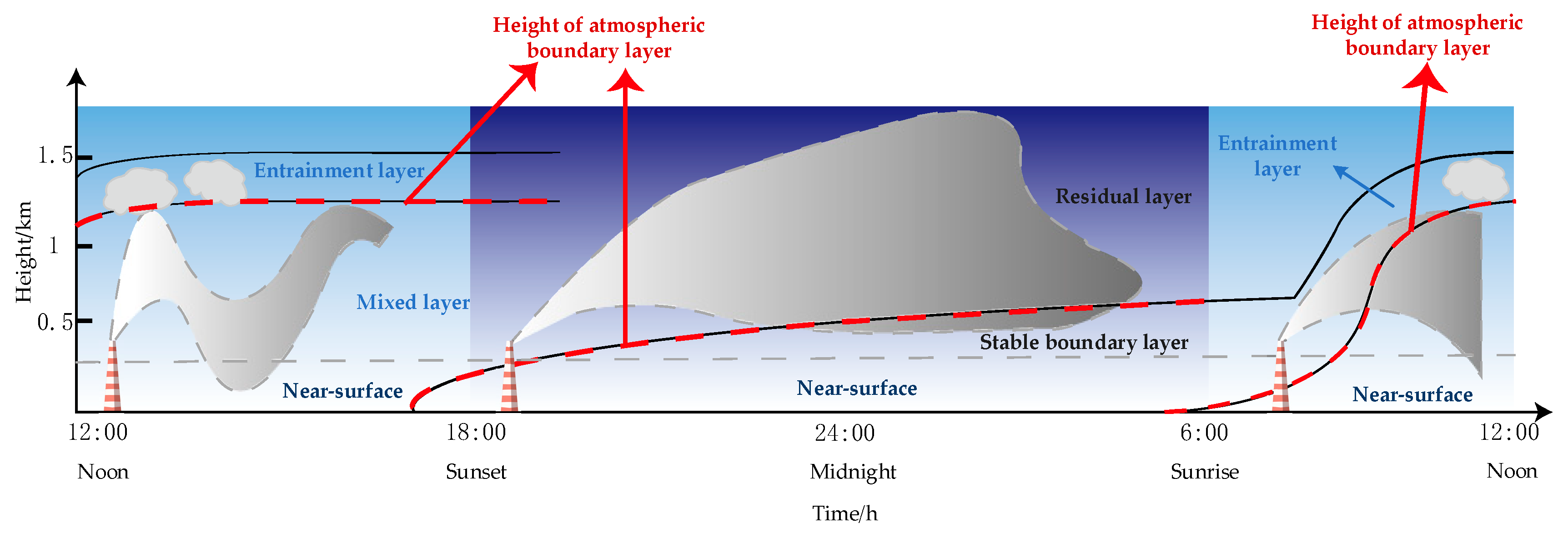
3.2. The STD Model of Air Pollutants Considering the Influence of ABL

The ABL undergoes significant diurnal variations throughout the day [58]. During the day, the intense radiation energy from the sun vigorously heats the Earth's surface, causing the temperature of the air layer in contact with the ground to rise. This process leads to the formation of a dynamic and active mixed layer (ML) near the surface, where the air undergoes vigorous mixing due to heat-induced rising and strong turbulent effects. Above this ML, a more stable entrainment layer (EL) forms, where air ascent and mixing are more pronounced. As the sun sets and night falls, the ground cools down due to the loss of solar radiation. This cooling effect renders the air near the ground colder and more stable, forming a stable boundary layer (SBL). The airflow in this layer is slower, and the vertical turbulent and mixing effects are reduced, facilitating the accumulation of pollutants near the surface. Above the SBL, there is the residual layer (RL), which retains some of the characteristics of the mixed layer formed during the day. Although the strong turbulence of the daytime has subsided, this layer level maintains certain mixing properties. As a result, the dispersion does not consistently adhere to a Gaussian distribution but manifests three typical pollutant diffusion forms: fumigation type, enclosed type, and downward inhibited type, as illustrated in Figure 3 [59].

$z_i$ refers to the bottom of the unstable ML. During the daytime, if $z_i$ has not exceeded $z_s$, the pollutants disperse following fumigation or enclosed type. After sunset, the SBL starts forming from the surface, while the daytime ML gradually transforms into a RL existing above the SBL. The ABL height $z_i$ is the height at the top of SBL, and pollutants disperse following the downward inhibited type [60].

3.2.1. Fumigation Type

Fumigation-type diffusion often occurs at night or in the early morning when the air temperature near the ground is lower than the air above due to radiative cooling, creating a temperature inversion layer. As a kind of air layer, the temperature inversion layer prevents pollutants near the ground from rising, leading to the accumulation of pollutants near the ground. Under these conditions, the pollutants exhibit a uniform distribution in the vertical direction and a Gaussian distribution in the horizontal direction. It can be expressed as: [50,61]

$$\left\{\begin{array}{l}{G}_i\left(\tau ,t^{\prime };x,y\right)=\frac{{\displaystyle {\int }_{-\infty }^m\exp }\left(-\frac{m^2}{2}\right)\mathrm{d}m\cdot \exp \left(-\frac{{\left(x-x_{\mathrm{c}}\left(\tau ,t^{\prime }\right)\right)}^2+{\left(y-y_{\mathrm{c}}\left(\tau ,t^{\prime }\right)\right)}^2}{2{\left({\sigma }_{y0}\left(\tau ,t^{\prime }\right)+\frac{z_{\mathrm{c}}\left(\tau ,t^{\prime }\right)}{8}\right)}^2}\right)}{{(2\pi )}^{\frac{3}{2}}{\left({\sigma }_{y0}\left(\tau ,t^{\prime }\right)+\frac{z_{\mathrm{c}}\left(\tau ,t^{\prime }\right)}{8}\right)}^2{z}_i(t)}\hfill \\ \hfill \left(L(\kappa )\ge 4|z_{\mathrm{s}}>z_i(\kappa )\right)\&L(\omega )<4)\\ m\left(t^{\prime }\right)=\frac{z_i(t)-z_{\mathrm{c}}\left(\tau ,t^{\prime }\right)}{{\sigma }_{z0}\left(\tau ,t^{\prime }\right)}\hfill \end{array}\right.$$

(32)

where $L(\omega )$ represents the atmospheric stability level below the height $z_i$ of the ABL at time $\tau$. $L(\omega )=4$ signifies neutrality. $\left(L(\kappa )\ge 4|z_{\mathrm{s}}>z_i(\kappa )\right)$ signifies the initial emission of pollutants within the stable layer. $L(\omega )<4$ denotes the formation of the ML. ${\sigma }_{y0}$ and ${\sigma }_{z0}$ represent the horizontal and vertical diffusion coefficients of pollutants initially within the stable layer. m stands for the operator.

3.2.2. Enclosed Type

This enclosed atmospheric pollutant diffusion generally occurs in the afternoon until before sunset during the day when the structure of the ABL exhibits stratification due to solar radiation heating. Under enclosed diffusion conditions, the ABL can be divided into two main parts: the upper EL and the lower ML. The EL has relatively stable meteorological conditions and can be seen as a “ceiling” that limits the upward diffusion of pollutants, making it difficult for pollutants to continue to penetrate upwards. Below the EL is the ML, where, due to the influence of ground heat radiation, air activity is frequent, aiding in the diffusion of pollutants both vertically and horizontally. During the enclosed atmospheric pollutant diffusion process, pollutants undergo continuous diffusion, reflection, and re-diffusion between these two levels, namely between the ground and the EL, creating a relatively closed diffusion environment. The expression can be represented as [62]:

$$\left\{\begin{array}{c}{G}_i\left(\tau ,t^{\prime };x,y\right)=\frac{\exp \left(-\frac{1}{2}{\left(\frac{x-x_{\mathrm{c}}\left(\tau ,t^{\prime }\right)}{{\sigma }_x\left(\tau ,t^{\prime }\right)}\right)}^2-\frac{1}{2}{\left(\frac{y-y_{\mathrm{c}}\left(\tau ,t^{\prime }\right)}{{\sigma }_y\left(\tau ,t^{\prime }\right)}\right)}^2\right)O\left(\tau ,t^{\prime }\right)}{{(2\pi )}^{\frac{3}{2}}{\sigma }_y^2\left(\tau ,t^{\prime }\right){\sigma }_z\left(\tau ,t^{\prime }\right)}\\ (L(\kappa )<4\&z_{\mathrm{s}}\le z_i(\kappa )\&L(\omega )<4)\\ O\left(\tau ,t^{\prime }\right)={\displaystyle \sum _{n=-N_{\mathrm{R}}}^{N_{\mathrm{R}}}\exp }\left(-\frac{{\left(2n{z}_i(t)-z_{\mathrm{c}}\left(\tau ,t^{\prime }\right)\right)}^2}{2{\sigma }_z^2\left(\tau ,t^{\prime }\right)}\right)+\\ {\displaystyle \sum _{n=-N_{\mathrm{R}}}^{N_{\mathrm{R}}}\exp }\left(-\frac{{\left(2n{z}_i(t)+z_{\mathrm{c}}\left(\tau ,t^{\prime }\right)\right)}^2}{2{\sigma }_z^2\left(\tau ,t^{\prime }\right)}\right)\end{array}\right.$$

(33)

where $L(\kappa )<4\&z_{\mathrm{s}}\le z_i(\kappa )\&L(\omega )<4$ denotes the puff that is emitted into the unstable ML. $L(\omega )<4$ denotes that the ABL still possesses a structure with the EL above and the ML below. $N_R$ represents the number of reflections of the pollutants’ puff, typically set at $N_R=4$ [63].

3.2.3. Downward Inhibited Type

After sunset, the ground receives weakened radiation, forming a neutral RL. As the night progresses, the RL bottom in direct contact with the ground gradually evolves into the SBL. Therefore, pollutants from the power plant are directly emitted into the RL at night. The pollutants spread equally in all directions, forming a cone-shaped diffusion profile. When the lower edge of the puff reaches the SBL, its downward diffusion begins to be inhibited, causing the distortion of the diffusion profile, hence referred to as downward-inhibited diffusion. The distortion of the diffusion profile is actually the variations in $y$ and $z$, which can be adjusted by modifying the values of α, β, λ, and γ and then correcting the puff dispersion coefficient based on Equation (29). During this period, the atmospheric stability condition is $L(\omega )\ge 4$, signifying that the pollutants are emitted into the SBL or the RL. The computation of the dispersion distribution function is as follows [57]:

$$\begin{array}{c}{G}_i\left(\tau ,t^{\prime };x,y\right)={\left[{(2\pi )}^{\frac{3}{2}}{\sigma }_y^2\left(\tau ,t^{\prime }\right){\sigma }_z\left(\tau ,t^{\prime }\right)\right]}^{-1}\cdot \exp \left(-\frac{1}{2}\left({\left(\frac{x-x_{\mathrm{c}}\left(\tau ,t^{\prime }\right)}{{\sigma }_x\left(\tau ,t^{\prime }\right)}\right)}^2+\right.\right.\\ \left.\left.{\left(\frac{y-y_{\mathrm{c}}\left(\tau ,t^{\prime }\right)}{{\sigma }_y\left(\tau ,t^{\prime }\right)}\right)}^2+{\left(\frac{z-z_{\mathrm{c}}\left(\tau ,t^{\prime }\right)}{{\sigma }_z\left(\tau ,t^{\prime }\right)}\right)}^2\right)\right)\end{array}$$

(34)

where ${\sigma }_x$, ${\sigma }_y$, and ${\sigma }_z$ are atmospheric pollutant diffusion parameters that have been adjusted according to Equation (25).

3.3. Discussions of the EED Model Considering the STD of Air Pollutant Emissions

Research on the STD of pollutants and their impact on the operation of the power system often involves the complex inter-relationships between multiple electrical and non-electrical source flows and the integration of multiple spatial and temporal levels. Research on the spatial and temporal constraints of various electrical and non-electrical composite source flows mainly focuses on two aspects: Firstly, the impact of electrical quantities on the distribution of atmospheric pollutants and non-electrical quantities, such as public health. This involves studying the “positive impact” of power system operation on the atmospheric environment. Secondly, there is a reverse driving process where the concentration of pollutants in living environments or non-electrical targets, such as the air quality index (AQI), influences the optimization dispatch of electricity. This constitutes “reverse pressure control” research, considering the impact of the atmospheric environment on power operation. The following discussion addresses two categories of research: the direct and indirect impacts of power system operation on the atmospheric environment.

3.3.1. Research on the Direct Impact of Power System Operation on the Atmospheric Environment

The operational mode of the power system primarily refers to its direct impact on the atmospheric environment, specifically influencing the distribution of regional air pollutant concentrations. In the 1970s, Sullivan R L and Hackett D Fi [44] introduced the characteristics of pollutant distribution into the optimization dispatch of power systems. They replaced the objective function of minimizing coal consumption with an objective function of minimizing the contribution of coal-fired units to the surface concentration of SO₂ at a specified location. As described in the previous section, the Gaussian plume dispersion model was utilized to calculate the contribution of unit emissions to the surface pollution concentration at the specified location. This led to the development of a “meteorology-sensitive” power dispatch plan. The results indicated that while the modeled system exhibited a slight increase in total SO₂ emissions, it effectively reduced the surface concentration of SO₂ at the specified location. The Gaussian plume model was also employed in [45], proposing an optimal decision model considering the pollutant diffusion process and meteorological conditions variations for high-sulfur and low-sulfur coal. Constraints were introduced into the model, including pollution concentration constraints at seven air quality monitoring points within urban communities. The concentration constraint of PM_2.5 was considered in [64], where the Gaussian plume model was employed to describe the dispersion of air pollutants around the load center. The results showed that it can effectively restrict the PM2.5 concentration at the load center compared to the seasonal management system. Chu K et al. [46,47] proposed an urban power dispatch method considering air quality constraints using the Gaussian plume model. The dynamic characteristics of pollutant diffusion were emphasized in [46], incorporating pollution concentration constraints into short-term economic dispatch plans and conducting simulation analysis in a power system with three power plants and three environmental monitoring points.

As international society gradually emphasizes environmental protection and atmospheric dispersion models such as CALPUFF [65] and CMAQ [66] become more mature, related research has advanced further. Dawar V. et al. [67] utilized the CMAQ dispersion model to simulate the distribution of PM_2.5 and ASO₄ concentrations resulting from unit-emitted SO₂ after secondary chemical transformations. They employed partial least squares techniques to sample the randomly generated outputs of the air quality model as constraints in the optimal power flow problem, aiming to enhance air quality. The commitment and dispatch model for power system units, taking into account air quality, was established in [68]. It incorporated robust optimization to ensure the pollutant concentration constraints. In [69], a comprehensive discussion was conducted on the “environmental coordinated dispatch” in the operation of power system dispatching, considering its mutual impact and synergy with the environmental system. It thoroughly analyzed the connotation and development of environmental coordinated dispatch, focusing on aspects such as environmentally sensitive power sources, multidimensional pollutant emission characteristics, and the impact patterns of pollutants on air quality. This discussion provided valuable insights for power dispatch, considering coordinated control with environmental meteorological conditions. The emission of various pollutants from coal-fired and gas-fired generators with different emission control devices was discussed in [70]. It proposed an environmental power generation dispatching model, taking into account the AQI and its weather influence, and optimized the spatial distribution of power generation between regions, balancing operational costs and the emissions of these pollutants. An approach to determine maintenance schedules for generating units based on AQI ranking results was presented in [71]. This method, involving the analysis of pollutant emissions and dispersion from coal-fired power units, can regulate the annual distribution of AQI contribution values from these units and alleviate air pollution levels during critical months. Li Z et al. [50] proposed an atmospheric pollutant dispersion model that considered both the temporal and spatial dimensions. In the temporal dimension, the model can coordinate multiple emission sources in the presence of atmospheric condition variations. In the spatial dimension, correlations between power plant siting, pollutant dispersion pathways, and the ABL were taken into account. The proposed model positively improved air quality, especially under adverse atmospheric conditions, where pollutant accumulation was significant and clean energy output was restricted across two distinct atmospheric conditions. Dai H et al. [72] proposed a high-dimensional multi-objective optimization dispatching strategy for power systems that considered the STD of multiple pollutants. The strategy encompassed models for the STD of pollutants, high-dimensional multi-objective optimization, multi-objective decision-making methods, and flexible dispatching based on environmental characteristics. By simultaneously reducing the generation cost, carbon emissions, and the impacts of VOCs, SO₂, and NO₂ on air quality, a balance was achieved between the reduction in generation cost and the impact on air quality. The multi-objective decision-making method filtered compromise solutions, effectively balancing the trade-off between cost reduction and environmental impact. Moreover, the flexible dispatching method allowed adjustments based on spatial and temporal variations in environmental capacity, enabling economically and environmentally friendly power dispatching.

In addition, some scholars have shifted the research focus to integrated energy systems, and utilizing clean energy sources such as natural gas and wind power is an effective way to reduce atmospheric pollution. The impacts of meteorological condition uncertainties on emission constraints were considered in [73], where a two-stage stochastic dispatching model was proposed. Wind power and energy storage can work together to help to reduce costs and/or emissions. The introduction of energy storage can balance the uncertainty of wind power, thus maintaining the balance of the grid’s power. Furthermore, it allowed for charging during periods of low pollution and discharging during periods of high pollution to meet emission restrictions during critical periods. In [74], an EED method was established for power-to-gas integrated systems, incorporating various emission controls. Traditional emission quantity control was applied to carbon emissions, while the STD was proposed for atmospheric pollutant emissions, considering ground concentrations and spatial environmental requirements. Two layers of convex dispersion optimization problems were presented, confirming the superiority of spatiotemporal diffusion control in reducing atmospheric pollutant concentrations. In [51], an EED strategy was proposed for coastal regional electrical and gas interconnected systems, considering the STD of pollutants, as well as power-to-gas integration. The study explored an atmospheric pollutant dispersion model considering local sea–land circulation and the coal-fired internal boundary layer. Addressing the increasing interdependence between power and natural gas systems, a new multi-objective optimal power-to-natural gas flow model with STD control was introduced in [75]. A convex-based generalized membership degree optimization method was employed to resolve target conflicts and non-convex gas transmission constraints, resulting in a high-quality solution.

3.3.2. Research on the Indirect Impacts of Power System Operation on the Atmospheric Environment

The operational mode of the power system has indirect impacts on the atmospheric environment, primarily referring to the adverse effects on population health and ecosystems within the atmospheric coverage zone. In the field of environmental engineering, research on the detrimental effects of power system emissions on population health often focuses on modeling the mapping relationship of “emission quantity-concentration distribution-health impacts”. The impacts of particulate matter, SO₂, and NO_x on health from an individual coal-fired power plant were estimated in [76]. In [77], the concept of intake fraction was introduced to assess the influence of emission source locations on the exposure of the population to fine particulate matter and sulfur dioxide. The CALPUFF atmospheric dispersion model was utilized to simulate the concentration distribution of air pollutants from 29 power plants in China. Based on a regression analysis considering regional climate, deposition capability, and population distribution, the intake fractions of pollutants such as inhalable PM and SO₂ for populations within different distances from power plants were determined. In [65], the CALPUFF model and meteorological data were applied to nine Illinois power plants to assess the impacts of primary and secondary particulate matter on the Midwest power grid. The results indicated that a significant population being influenced by long-distance transport and emissions from power plants across the United States may have substantial implications for public health. The CMAQ-RSM model was employed in [78] to simulate the distribution of PM_2.5 concentration changes in various US cities due to pollution source reduction. Subsequently, corresponding population health costs were calculated. The relationship between PM_2.5 concentration in the air and population epidemiology was discussed in [79], revealing positive correlations with the overall mortality rate, cardiovascular mortality rate, and lung cancer mortality rate based on environmental PM_2.5 concentration.

Currently, few power dispatch models take into account the adverse effects of coal-fired unit emissions on population health. In [80], a simulation was conducted to monetize damages associated with 407 coal-fired power plants in the United States. This consideration of unit emissions enabled the identification of more efficient control strategies that accounted for the variability in damage across facilities, ultimately contributing to the design of optimal energy policy and the evaluation of competing fuels for electricity generation. Lei S et al. [81] calculated unit emissions’ population health costs by considering population and AQI levels. They introduced penalty costs into the objective function of the unit combination model and utilized robust optimization to adapt to the uncertainty of wind power. Kerl P Y et al. [82] utilized the CMAQ-DDM dispersion model and health functions to establish a response function for unit emissions and population health costs. Taking into account the goal of power generation cost, the results indicated that the developed dispatch strategy could save 175.9 million US dollars in health costs for the state of Georgia from 2004 to 2011. Ban M et al. [83] computed the population health impacts of unit emissions, establishing a combination model incorporating wind power and energy storage while considering differentiated population health effects. Additionally, they addressed the optimal charging and discharging paths for electric vehicles, further enhancing the model’s effectiveness [84].

In summary, through the study of atmospheric dispersion models, a more accurate understanding of the spread patterns of pollutants in the air can be obtained, providing real-time and precise environmental data for electric power dispatch decision-making. The robustness of the air quality monitoring network allows for comprehensive monitoring of air quality conditions in different regions, enabling the timely detection and addressing of potential environmental issues. Consequently, advancements in atmospheric dispersion models and air quality monitoring networks inject new vitality into the field of power dispatch, laying a solid foundation for achieving a clean and sustainable power supply. Simultaneously, an in-depth exploration of two types of research focusing on the direct and indirect impacts of the power system’s operational mode on the atmospheric environment allows for a more comprehensive understanding of the inter-relationship between the power system and the environment. This, in turn, provides scientific support for the intelligent and sustainable development of future power systems.

4. Solution Methods for the EED Models

Section 2 and Section 3 introduce different models of EED. To significantly improve the performances of these EED models and ensure that the power system operates both cleanly and efficiently, various optimization strategies have been applied to solve the EED challenges while complying with environmental and sustainable development standards. These strategies fall into three categories: (i) conventional methods, (ii) non-conventional methods, and (iii) hybrid methods.

4.1. Conventional Methods

Conventional mathematical programming methods for solving the EED models include Lagrangian relaxation [85], linear programming [86,87], dynamic programming [88], quadratic programming [89,90], $\lambda$-iteration [91], Newton–Raphson [92], the interior point method [93], and weighted extremum-seeking [94]. Conventional methods have certain advantages, such as their lack of problem-specific parameters [95], mathematically proven optimality [21], and faster convergence for smaller system sizes [20]. However, these methods also have corresponding drawbacks. For instance, the dynamic programming method is prone to the curse of dimensionality, and linear programming may lose accuracy when solving nonlinear objective functions. Additionally, when using mathematical programming methods, the impact of initial values on the solution is sensitive, making algorithms susceptible to local optima. Moreover, these methods typically require the differentiability of the objective function, and if the objective function is non-convex (due to effects like valve-point loading in coal-fired power units or prohibited zones), it may lead to unsolvability issues.

4.2. Non-Conventional Methods

In recent decades, numerous unconventional methods based on artificial intelligence have been widely utilized to address the constraints associated with conventional methods based on mathematical models when solving the EED problems. These unconventional approaches, including the genetic algorithm (GA), the particle swarm optimization algorithm (PSO), and other artificial intelligence algorithms, have fewer restrictions compared to mathematical programming methods. This flexibility allows them to solve objective functions characterized by nonlinearity and non-convexity effectively.

4.2.1. GA Method

GA is an optimization and search algorithm inspired by natural selection [96]. It is used to find solutions to complex problems by mimicking the principles of genetics and evolution. It has been applied by Koridak et al. [97] and employed to determine the fuel cost and the function of emission gas in the electric power network, optimizing the fuel cost of production and the quantities of emission gases in the environment at the same time. Srinivas N et al. [98] proposed a method utilizing non-dominated sorting in genetic algorithms to address multi-objective optimization problems. They applied this approach to three dual-objective test problems. However, the non-dominated sorting genetic algorithm-II for solving combined heat and power economic emission dispatch problem was proposed in [99], providing a competitive performance in terms of solution quality. Abido M A [100] introduced an approach based on the niched Pareto genetic algorithm (NPGA) to address the multi-objective EED problem. A key benefit of this method is its lack of constraints on the number of optimized objectives. In [101], a lambda-based hybrid genetic algorithm was employed to solve the EED problem. The real-coded genetic algorithm was utilized for global search, and Tabu Search conducted fine-tunings to guide the search toward the optimal region and ensure local optimization.

4.2.2. PSO Method

PSO is a swarm intelligence algorithm inspired by collective behaviors observed in organisms such as flocks of birds and schools of fish. It was initially proposed by James Kennedy and Russell Eberhart in 1995 [102]. The fundamental idea of PSO is to search for the optimal solution to a problem by simulating cooperation and information sharing between individuals in a swarm. Ratniyomchai T et al. applied the PSO algorithm to a dual-objective optimization problem involving the minimization of both fuel costs and pollutant emissions [23]. They achieved a well-distributed Pareto frontier. Kheshti M et al. [103] proposed double-weighted particle swarm optimization (DWPSO) to address wind power penetration in non-convex combined emission economic dispatch and non-convex multi-fuel selection economic dispatch problems. Zhang et al. utilized a bare-bones multi-objective particle swarm optimization (BB-MOPSO) to address optimization problems in the EED problem. The algorithm, requiring no adjustment of control parameters in the particle update strategy, incorporated a time-varying mutation operator to enhance search capabilities [104]. Hadji B et al. proposed a PSO algorithm based on time-varying acceleration (PSO-TVAC), dynamically adjusting acceleration coefficients during the search process to balance exploration and exploitation abilities, thereby improving the performance of the standard PSO algorithm [105]. Rezaie H et al. proposed an advanced particle swarm optimization (APSO) to solve the EED problem considering transmission losses, valve-point loading effects, ramp rate limits, and prohibited operating zones [106]. Zuo et al. introduced a new global particle swarm optimization (NGPSO) to address carbon emission and cost optimization problems. This algorithm balanced the minimization of fuel costs and emissions with the requirements of power balance and generation limits [107].

4.2.3. Other Artificial Intelligence Algorithm Methods

In [22], a differential evolution (DE) algorithm was developed to solve emission-constrained economic power dispatch problems. Sharma R et al. [108] presented a multi-objective differential evolution algorithm (MODE) to solve a nonlinear constrained multi-objective problem with the competing and non-commensurable objectives of fuel cost and emission. Yu X et al. [109] improved conventional DE by employing two mutation strategies: DE/rand/1 and DE/current-to-rand/1. In [110], an enhanced multi-objective differential evolution algorithm (EMODE) was proposed. This algorithm enhanced optimization performance by incorporating the advantages of two selection strategies: feasible solution and non-dominated sorting. It combined total constraint violation and penalty functions to handle various constraints, providing better dynamic dispatching solutions for power systems.

Almost simultaneously, Ramesh et al. [111] and Nikman T et al. [112] proposed the bat algorithm (BA) for solving the EED problems. Nikman T et al. [112] employed a metaheuristic BA to achieve the Pareto optimal solution set. This algorithm incorporated a novel adaptive learning approach, enhancing the diversity of the population and refining the convergence criteria.

In 2011, a multi-objective teaching–learning-based optimization algorithm (TLBO) with non-domination based sorting was applied to solve the EED problem [113]. Niknam T et al. [114] proposed the θ-teaching–learning-based optimization (θ-TLBO) algorithm based on the TLBO algorithm. In this proposed method, the optimization process was based on phase angles rather than the design variables themselves. This approach more effectively considered the nonlinear characteristics of the problem and avoided falling into local optima. It was compared with algorithms such as GA and PSO, demonstrating its superior solving efficiency.

Other artificial intelligence algorithms such as the firefly algorithm (FFA) [115], simulated annealing (SA) [116,117], the gravitational search algorithm (GSA) [118], grey wolf optimization (GWO) [119,120], and artificial bee colony (ABC) [121,122] have also played crucial roles in addressing the EED model.

Table 6. Summary of non-conventional methods related to the EED problems.

Author/Year	Methods	Single-Objective or Multi-Objective Optimization	Objective(s)
Basu, M. (2005) [116]	SA	Multi-objective	[Generation cost, Emission cost]
Koridak, L.A. et al. (2008) [97]	GA	Single-objective	Generation cost, Emission cost
Ratniyomchai, T. et al. (2010) [23]	PSO	Multi-objective	[Generation cost, Emission cost]
Abou El Ela, A. et al. (2010) [22]	DE	Single-objective	Generation cost
Krishnanand, K. et al. (2011) [113]	TLBO	Multi-objective	[Generation cost, Emission cost]
Niknam, T. et al. (2012) [114]	θ-TLBO	Multi-objective	[Generation cost, Emission cost]
Chandrasekaran, K. et al. (2012) [115]	FFA	Multi-objective	[Generation cost, Emission cost, The reliability of the system]
Güvenc, U. et al. (2012) [118]	GSA	Multi-objective	[Generation cost, Emission cost]
Zhang, Y. et al. (2012) [104]	BB-MOPSO	Multi-objective	[Generation cost, Emission cost]
Basu, M. (2013) [99]	NSGA-II	Multi-objective	[Combined heat and power generation cost, Emission costs for SO2 and NOx]
Niknam, T. et al. (2013) [112]	BA	Multi-objective	[Generation cost, Emission cost]
Hadji, B. et al. (2015) [105]	PSO-TVAC	Multi-objective	[Generation cost, Emission cost]
Chopra, N. et al. (2016) [119]	GWO	Multi-objective	[Combined heat and power generation cost, Emission costs for SO2, CO2, and NOx]
Zou, D. et al. (2017) [107]	NGPSO	Multi-objective	[Generation cost, Emission cost]
Kheshti, M. et al. (2018) [103]	DWPSO	Single-objective	[Generation cost, Emission cost]
Abdullah, M. et al. (2018) [121]	ABC	Multi-objective	[Generation cost, Emission cost]
Bai, Y. et al. (2021) [110]	EMODE	Multi-objective	[Generation cost, Emission cost]

presents a summary of non-conventional methods related to the EED problems.

Each individual algorithm has its strengths and weaknesses. Combining different algorithms can effectively enhance solution efficiency and accuracy, thus introducing hybrid algorithms.

4.3. Hybrid Methods

Hybrid methods combine two or more different types of algorithms or techniques. With characteristics such as strong adaptability, handling diverse data, and improving robustness, hybrid algorithms can effectively overcome the limitations of a single algorithm, providing a more comprehensive solution for complex problems. In [123], a hybrid multi-objective optimization algorithm based on PSO and DE was proposed. In this algorithm, a particle swarm with a time-varying acceleration coefficient was designed to explore the entire search space, and a local version of the particle swarm was introduced to exploit sparse solutions in developing subspaces. In [124], a hybrid approach combining the bacterial foraging (BF) algorithm with the Nelder–Mead (NM) algorithm (BF-NM algorithm) was employed to solve the EED problem. The objective function of this problem simultaneously considered generation, spinning reserve, and emission costs. Various constraints such as frequency deviation, minimum frequency limit, ramp rate limit, transmission line losses, maximum emission limits for specific power plants or the entire power system, prohibited operating zones, and frequency constraints were also taken into account. Performance comparison with other intelligent algorithms such as PSO, GA, DE, and BF algorithm reveals the superiority of this method for reducing the overall system cost. Jiang S et al. [125] proposed a hybrid algorithm called the hybrid particle swarm optimization and gravitational search algorithm (HPSO-GSA), which incorporated features of both PSO and GSA. The algorithm employed cooperative evolution techniques, synchronizing particle positions with the particle swarm velocity and acceleration updates. When compared with algorithms such as PSO, GSA, MODE, and NSGA-II, the proposed method demonstrated its potential and effectiveness.

Recently, based on the rapid convergence of the DE algorithm and the particle diversity of the GA crossover operator, Zhao et al. [126] proposed a differential evolution-crossover quantum particle swarm optimization (DE-CQPSO) algorithm. To achieve better optimization results, a parameter adaptive control method was employed to update the crossover probability. A penalty factor was introduced to address multi-objective optimization problems. The results indicated that the evaluation metrics and convergence speed of the DE-CQPSO algorithm outperformed algorithms such as quantum particle swarm optimization (QPSO) and NGPSO, whether in terms of single-objective fuel cost and emission optimization or multi-objective optimization considering both objectives. In [127], a hybrid optimization algorithm based on the weighted vertex optimizer and particle swarm optimization (WVO-PSO) method was proposed for solving environment economic dispatch, combined heat and power economic dispatch, and combined heat and power environment economic dispatch problems. Ellahi M et al. [24] proposed a modified hybrid PSO algorithm with a BA parameter inspiration acceleration coefficient (MHPSO-BAAC). The algorithm’s performance was validated by solving the EEDs of all RES-based power systems under three conditions: unconstrained, time-varying demand, and regional load-sharing dispatch. Dashtdar M et al. [128] proposed a combination of the FFA and GA to solve the EED problem among coal-fired power plants. This approach took into account nonlinear constraints such as the valve effect, generation-restricted zones, and generation variation rates. Bhargava G and Yadav N K [129] utilized a hybrid algorithm combining the crow search and differential evolution algorithms (CSA-DE) to balance emission and economic costs. In [130], a multi-objective Multi-Verse Optimization Algorithm Based on Gridded Knee Points and Plane Measurement (GKPPM-MVO) technique was proposed. This algorithm demonstrates good adaptability and also provides a greater number of Pareto solutions. Chandrashekhar M et al. [131] proposed the Honey Bee Simulated Annealing (HB-SA) algorithm to concurrently address the load flow analysis and the economic and emission dispatch problem while accommodating valve point loading effects. This approach provided a novel method for addressing the complex power flow issues inherent in the EED problem, presenting a compelling strategy for resolving power system challenges. A short summary of hybrid methods related to the EED problems is presented in

Table 7. Summary of hybrid methods related to the EED problems.

Author/Year	Methods	Single-Objective or Multi-Objective Optimization	Objective(s)
Gong, D. et al. (2010) [123]	MO-DE/PSO	Multi-objective	[Generation cost, Emission cost]
Hooshmand, R.-A. et al. (2012) [124]	BF-NM	Multi-objective	[Generation cost, Emission cost, Power plant spinning reserve cost]
Jiang, S. et al. (2014) [125]	HPSO-GSA	Multi-objective	[Generation cost, Emission cost]
Zhao et al. (2020) [126]	DE-CQPSO	Multi-objective	[Generation cost, Emission cost]
Dolatabadi, S. et al. (2020) [127]	WVO-PSO	Multi-objective	[Generation cost, Emission cost]
Ellahi, M. et al. (2021) [24]	MHPSO-BAAC	Multi-objective	[Generation cost, Emission cost, RES production cost]
Dashtdar, M. et al. (2022) [128]	FFA-GA	Multi-objective	[Generation cost, Emission cost]
Bhargava, G. et al. (2022) [129]	CSA-DE	Multi-objective	[Generation cost, Emission cost]
Xu, W. et al. (2023) [130]	GKPPM-MVO	Multi-objective	[Generation cost, Emission cost]
Chandrashekhar, M. et al. (2024) [131]	HB-SA	Multi-objective	[Generation cost, Emission cost]

.

5. Research on the Multi-Area EED Models

The EED models discussed above optimize the atmospheric environmental objectives for a specific region. However, differences in the economy and environment across various regions suggest that employing multi-area dispatch can lead to efficient power distribution, reduce system operational costs, and alleviate the level of atmospheric pollution in high-pollution areas [132,133]. Currently, research on optimization dispatch that considers the environmental mutual benefits of multi-area power grids is relatively scarce and can generally be classified into two categories: economic dispatch that minimizes pollutant emissions within each region or across the entire grid and economic dispatch that takes into account the environmental factors of each region. In [134,135], a multi-area power grid environmental economic dispatch model was established with the objective functions of overall network economic efficiency and environmental friendliness. Jadoun V K et al. [136] proposed an enhanced particle swarm optimization method to address the multi-area environmental economic dispatch problem with reserve constraints. In [137], the objective of the multi-area EED problem was to establish an optimal plan for the operation of coal-fired power generation units in different regions of the power system and determine power transfers between regions to minimize the overall system operating costs and emissions. The multi-area EED problem was solved in two stages. In the first stage, the optimal power of the generators was determined to minimize costs and emissions, considering unit operation within a single region. In the second stage, starting from the results obtained in the first stage, the transfer of power between regions was determined to ensure power balance in each region of the analyzed system.

The aforementioned research provides an effective solution for controlling the total pollution emissions in multi-area power grids. However, it lacks consideration of environmental factors such as AQI indicators and population health impacts in densely populated areas within each region. Following the principle of “regional optimization, inter-regional coordination”, Guo D et al. [138,139] established a day-ahead power dispatching model for regional power grids with environmental benefit optimization and a multi-area power grid coordination model to enhance environmental mutual assistance benefits. Incentives for green certificates during heavy pollution weather encouraged the substitution of clean electricity across regions. Simultaneously, by adjusting the interconnection line plans, surplus atmospheric environmental capacity in one region’s power grid supports power supplied to regions facing heavy pollution. The results indicated that the proposed strategies effectively alleviated heavy pollution weather conditions in densely populated areas.

6. Discussion and Future Directions

The authors have conducted extensive searches and surveys on the issue of EED. The retrieved content includes the EED model considering TAPC, where most of the literature focuses on technological innovation through research on optimization algorithms. Another part of the literature studies the EED model based on the optimization of the STD of air pollutant emissions, primarily focusing on the establishment of gas diffusion models. This paper organizes and summarizes these two parts of the literature, providing convenient technical support for relevant researchers.

The EED model considering TAPC is suitable for establishing more general macro-level generation planning for power systems. Similar models can also be applied to economic dispatch models that control carbon emissions because controlling CO₂ emissions from the perspective of total emissions can effectively mitigate global warming. The EED model based on the optimization of the STD of air pollutant emissions takes into full consideration the influence of diurnal variations in the ABL, employing a more precise approach to constrain the GPLC, thereby achieving sustainable development, both environmentally and economically. Section 4 introduces three categories of methods for solving EED problems. Although each method has its pros and cons, in recent years, researchers have shown a growing interest in the development and use of hybrid methods to address EED problems, aiming to harness the advantages of different methods and overcome their respective shortcomings. After discussing EED models for specific areas, this paper further expands and summarizes the current state of and methods for existing multi-area EED model research, with the goal of making flexible power dispatch decisions based on the atmospheric pollution tolerance conditions of different areas.

Despite this, the EED models discussed in this paper still have certain limitations. When introducing models of the STD of atmospheric pollutants, they failed to fully consider the influence of meteorological factors such as rainfall and air humidity, nor did they consider the constraints of topographical conditions [50]. In practice, the STD of atmospheric pollutants is a complex physical model influenced by various uncertainties, and traditional modeling approaches may not fully align with real-world situations. In recent years, the rise of artificial intelligence has had significant implications for the fields of electricity and the atmospheric environment. It can be utilized not only for optimization solutions but also to guide the dispatching of power systems, enhancing the efficiency, reliability, and stability of power systems [140,141,142,143]. In the atmospheric environment domain, artificial intelligence algorithms can be employed for meteorological data analysis and climate model development, providing a better understanding of climate change trends [144,145,146]. Consequently, applying artificial intelligence algorithms to the EED model is poised to become a future trend. At the same time, with the large-scale integration of renewable energy into the power grid, although environmental issues have seen improvements, the inherent uncertainty of renewable energy sources has led to increased volatility in the power system, making it difficult to achieve stable electricity supply [147]. This has added to the complexity of power system dispatch, and it may be necessary to consider a variety of reserve and flexibility resources to balance supply and demand, thereby improving the reliability of the power system [148,149,150]. It is essential to consider that when factoring in backup resources such as energy storage and flexibility resources like electric vehicles, the environmental impact of battery aging must also be taken into account [151,152]. The broader strategy for managing pollution within the power system requires careful planning from a macroscopic viewpoint, a topic that extends beyond the scope of this discussion. In conclusion, future EED models that integrate a variety of renewable energy sources along with diverse backup and flexible resources hold the promise of unlocking the potential for greener power dispatch. This approach has extensive application potential and could lead to significant advancements in the field.

7. Conclusions

This paper aims to summarize and synthesize the existing EED models and their solutions. Two types of single-area EED models with different control strategies, solution methods, multi-area EED models, discussion, and future directions have been covered.

While there have been several articles summarizing the EED models, most of them have only focused on summarizing and comparing the solution algorithms of the model, neglecting the discussion on the distinction between total pollutant control and ground-level pollutant concentration control. Furthermore, while summarizing the EED models, this article identifies certain limitations: there is a lack of research on multi-area EED problems that dispatch separately for densely populated and sparsely populated areas; existing atmospheric pollutant dispersion models neglect natural conditions such as rainfall, humidity, and terrain; and there is scarce consideration of the coordinated EED involving the uncertainties of renewable energy sources and a variety of flexible resources. Conducting further in-depth research on such models is of significant importance for the improvement of public welfare and government management. Ultimately, it also provides a variety of novel dispatch strategies for the actual power grid’s EED, carrying considerable theoretical and practical value.

References

1. World Health Organization. WHO Global Air Quality Guidelines: Particulate Matter (PM2. 5 and PM10), Ozone, Nitrogen Dioxide, Sulfur Dioxide and Carbon Monoxide; World Health Organization: Geneva, Switzerland, 2021; ISBN 92-4-003422-6.
2. Velasco, R.P.; Jarosińska, D. Update of the WHO global air quality guidelines: Systematic reviews–An introduction. Environ. Int. 2022, 170, 107556. [Google Scholar] [CrossRef]
3. Zhang, H.; Sun, C.; Ge, M. Review of the research status of cost-effective zinc–iron redox flow batteries. Batteries 2022, 8, 202. [Google Scholar] [CrossRef]
4. Boretti, A.; Castelletto, S. Hydrogen energy storage requirements for solar and wind energy production to account for long-term variability. Renew. Energy 2024, 221, 119797. [Google Scholar] [CrossRef]
5. Wolniak, R.; Skotnicka-Zasadzień, B. Development of Wind Energy in EU Countries as an Alternative Resource to Fossil Fuels in the Years 2016–2022. Resources 2023, 12, 96. [Google Scholar] [CrossRef]
6. Zhang, G.-X.; Yang, Y.; Su, B.; Nie, Y.; Duan, H.-B. Electricity production, power generation structure, and air pollution: A monthly data analysis for 279 cities in China (2015–2019). Energy Econ. 2023, 120, 106597. [Google Scholar] [CrossRef]
7. Liu, Y.; Li, X.; Liu, Y. A Low-Carbon and Economic Dispatch Strategy for a Multi-Microgrid Based on a Meteorological Classification to Handle the Uncertainty of Wind Power. Sensors 2023, 23, 5350. [Google Scholar] [CrossRef] [PubMed]
8. Luo, Q.; Garcia-Menendez, F.; Yang, H.; Deshmukh, R.; He, G.; Lin, J.; Johnson, J.X. The health and climate benefits of economic dispatch in China’s power system. Environ. Sci. Technol. 2023, 57, 2898–2906. [Google Scholar] [CrossRef] [PubMed]
9. Cai, W.; Wang, C.; Wang, K.; Zhang, Y.; Chen, J. Scenario analysis on CO2 emissions reduction potential in China’s electricity sector. Energy Policy 2007, 35, 6445–6456. [Google Scholar] [CrossRef]
10. Zhang, N.; Kang, C.; Kirschen, D.S.; Xia, Q.; Xi, W.; Huang, J.; Zhang, Q. Planning pumped storage capacity for wind power integration. IEEE Trans. Sustain. Energy 2012, 4, 393–401. [Google Scholar] [CrossRef]
11. Mirzaesmaeeli, H.; Elkamel, A.; Douglas, P.L.; Croiset, E.; Gupta, M. A multi-period optimization model for energy planning with CO2 emission consideration. J. Environ. Manag. 2010, 91, 1063–1070. [Google Scholar] [CrossRef] [PubMed]
12. Li, J.F.; Wang, X.; Zhang, Y.X.; Kou, Q. The economic impact of carbon pricing with regulated electricity prices in China—An application of a computable general equilibrium approach. Energy Policy 2014, 75, 46–56. [Google Scholar] [CrossRef]
13. Hammoudeh, S.; Lahiani, A.; Nguyen, D.K.; Sousa, R.M. An empirical analysis of energy cost pass-through to CO2 emission prices. Energy Econ. 2015, 49, 149–156. [Google Scholar] [CrossRef]
14. Bhanarkar, A.D.; Purohit, P.; Rafaj, P.; Amann, M.; Bertok, I.; Cofala, J.; Rao, P.S.; Vardhan, B.H.; Kiesewetter, G.; Sander, R. Managing future air quality in megacities: Co-benefit assessment for Delhi. Atmos. Environ. 2018, 186, 158–177. [Google Scholar] [CrossRef]
15. Shi, Q.; Zheng, B.; Zheng, Y.; Tong, D.; Liu, Y.; Ma, H.; Hong, C.; Geng, G.; Guan, D.; He, K. Co-benefits of CO2 emission reduction from China’s clean air actions between 2013–2020. Nat. Commun. 2022, 13, 5061. [Google Scholar] [CrossRef]
16. Lu, Z.; Huang, L.; Liu, J.; Zhou, Y.; Chen, M.; Hu, J. Carbon dioxide mitigation co-benefit analysis of energy-related measures in the Air Pollution Prevention and Control Action Plan in the Jing-Jin-Ji region of China. Resour. Conserv. Recycl. X 2019, 1, 100006. [Google Scholar] [CrossRef]
17. Pandit, N.; Tripathi, A.; Tapaswi, S.; Pandit, M. An improved bacterial foraging algorithm for combined static/dynamic environmental economic dispatch. Appl. Soft Comput. 2012, 12, 3500–3513. [Google Scholar] [CrossRef]
18. Carrillo-Galvez, A.; Flores-Bazan, F.; Lopez, E. A duality theory approach to the environmental/economic dispatch problem. Electr. Power Syst. Res. 2020, 184, 106285. [Google Scholar] [CrossRef]
19. Zhu, L.; Ren, H.; Habibi, M.; Mohammed, K.J.; Khadimallah, M.A. Predicting the environmental economic dispatch problem for reducing waste nonrenewable materials via an innovative constraint multi-objective Chimp Optimization Algorithm. J. Clean. Prod. 2022, 365, 132697. [Google Scholar] [CrossRef]
20. Pandian, S.M.V.; Thanushkodi, K.; Anjana, P.S.; Dilesh, D.; Kiruthika, B.; Ramprabhu, C.S.; Vibinth, A. An efficient particle swarm optimization technique to solve combined economic emission dispatch problem. Eur. J. Sci. Res. 2011, 54, 187–192. [Google Scholar]
21. Bansal, R.C. Optimization methods for electric power systems: An overview. Int. J. Emerg. Electr. Power Syst. 2005, 2, 1021. [Google Scholar] [CrossRef]
22. Abou El Ela, A.A.; Abido, M.A.; Spea, S.R. Differential evolution algorithm for emission constrained economic power dispatch problem. Electr. Power Syst. Res. 2010, 80, 1286–1292. [Google Scholar] [CrossRef]
23. Ratniyomchai, T.; Oonsivilai, A.; Pao-La-Or, P.; Kulworawanichpong, T. Particle swarm optimization for solving combined economic and emission dispatch problems. In Proceedings of the 5th IASME/WSEAS International Conference on Energy & Environment, Stevens Point, WI, USA, 23–25 February 2010; pp. 211–216. [Google Scholar]
24. Ellahi, M.; Abbas, G.; Satrya, G.B.; Usman, M.R.; Gu, J. A modified hybrid particle swarm optimization with bat algorithm parameter inspired acceleration coefficients for solving eco-friendly and economic dispatch problems. IEEE Access 2021, 9, 82169–82187. [Google Scholar] [CrossRef]
25. Talaq, J.; El-Hawary, F.; El-Hawary, M. A summary of environmental/economic dispatch algorithms. IEEE Trans. Power Syst. 1994, 9, 1508–1516. [Google Scholar] [CrossRef]
26. Qu, B.Y.; Zhu, Y.S.; Jiao, Y.C.; Wu, M.Y.; Suganthan, P.N.; Liang, J.J. A survey on multi-objective evolutionary algorithms for the solution of the environmental/economic dispatch problems. Swarm Evol. Comput. 2018, 38, 1–11. [Google Scholar] [CrossRef]
27. Mahdi, F.P.; Vasant, P.; Kallimani, V.; Watada, J.; Fai, P.Y.S.; Abdullah-Al-Wadud, M. A holistic review on optimization strategies for combined economic emission dispatch problem. Renew. Sustain. Energy Rev. 2018, 81, 3006–3020. [Google Scholar] [CrossRef]
28. Marouani, I.; Guesmi, T.; Hadj Abdallah, H.; Alshammari, B.M.; Alqunun, K.; Alshammari, A.S.; Rahmani, S. Combined Economic Emission Dispatch with and without Consideration of PV and Wind Energy by Using Various Optimization Techniques: A Review. Energies 2022, 15, 4472. [Google Scholar] [CrossRef]
29. Gent, M.; Lamont, J.W. Minimum-emission dispatch. IEEE Trans. Power Appar. Syst. 1971, PAS-90, 2650–2660. [Google Scholar] [CrossRef]
30. Lu, Y.; Zhou, J.; Qin, H.; Wang, Y.; Zhang, Y. A hybrid multi-objective cultural algorithm for short-term environmental/economic hydrothermal scheduling. Energy Convers. Manag. 2011, 52, 2121–2134. [Google Scholar] [CrossRef]
31. Guo, C.; Bai, Y.; Zheng, X.; Zhan, J.; Wu, Q. Optimal generation dispatch with renewable energy embedded using multiple objectives. Int. J. Electr. Power Energy Syst. 2012, 42, 440–447. [Google Scholar] [CrossRef]
32. Wang, A.C.; Pan, W.G.; Wang, W.H. A study of multi-objective load optimal dispatch in thermal power unit based on improved particle swarm optimization algorithm. Adv. Mater. Res. 2014, 860, 1425–1430. [Google Scholar] [CrossRef]
33. Chandrasekaran, K.; Simon, S.P. Multi-objective unit commitment problem with reliability function using fuzzified binary real coded artificial bee colony algorithm. IET Gener. Transm. Distrib. 2012, 6, 1060–1073. [Google Scholar] [CrossRef]
34. Subbaraj, P.; Rengaraj, R.; Salivahanan, S. Enhancement of self-adaptive real-coded genetic algorithm using Taguchi method for economic dispatch problem. Appl. Soft Comput. 2011, 11, 83–92. [Google Scholar] [CrossRef]
35. Park, J.-B.; Jeong, Y.-W.; Shin, J.-R.; Lee, K.Y. An improved particle swarm optimization for nonconvex economic dispatch problems. IEEE Trans. Power Syst. 2009, 25, 156–166. [Google Scholar] [CrossRef]
36. Cai, J.; Li, Q.; Li, L.; Peng, H.; Yang, Y. A hybrid FCASO-SQP method for solving the economic dispatch problems with valve-point effects. Energy 2012, 38, 346–353. [Google Scholar] [CrossRef]
37. Fraga, E.S.; Yang, L.; Papageorgiou, L.G. On the modelling of valve point loadings for power electricity dispatch. Appl. Energy 2012, 91, 301–303. [Google Scholar] [CrossRef]
38. Hannun, R.M.; Razzaq, A.H.A. Air Pollution Resulted from Coal, Oil and Gas Firing in Thermal Power Plants and Treatment: A Review. In IOP Conference Series: Earth and Environmental Science, Proceedings of the First International Scientific Conference on the Environment of Marshes and Water Surfaces (ISCEMWS-2021), Nasiriyah, Iraq, 17–18 November 2021; IOP Publishing: Bristol, UK, 2022; Volume 1002, p. 012008. [Google Scholar]
39. Wang, G.; Deng, J.; Zhang, Y.; Zhang, Q.; Duan, L.; Hao, J.; Jiang, J. Air pollutant emissions from coal-fired power plants in China over the past two decades. Sci. Total Environ. 2020, 741, 140326. [Google Scholar] [CrossRef]
40. Zhao, B.; Guo, C.; Cao, Y. Dynamic economic dispatch in electricity market using particle swarm optimization algorithm. In Proceedings of the Fifth World Congress on Intelligent Control and Automation (IEEE Cat. No.04EX788), Hangzhou, China, 15–19 June 2004; Volume 6, pp. 5050–5054. [Google Scholar]
41. Bouktir, T.; Labdani, R.; Slimani, L. Economic power dispatch of power system with pollution control using multiobjective particle swarm optimization. J. Pure Appl. Sci. 2007, 4, 57–77. [Google Scholar]
42. Lu, S.; Makarov, Y.V.; Zhu, Y.; Lu, N.; Kumar, N.P.; Chakrabarti, B.B. Unit commitment considering generation flexibility and environmental constraints. In Proceedings of the IEEE PES General Meeting, Minneapolis, MN, USA, 25–29 July 2010; pp. 1–11. [Google Scholar]
43. Wu, L.; Shahidehpour, M.; Li, T. Stochastic security-constrained unit commitment. IEEE Trans. Power Syst. 2007, 22, 800–811. [Google Scholar] [CrossRef]
44. Sullivan, R.L.; Hackett, D.F. Air quality control using a minimum pollution-dispatching algorithm. Environ. Sci. Technol. 1973, 7, 1019–1022. [Google Scholar] [CrossRef]
45. Chen, Y. Optimal Environmental Economic Power Dispatch Considering Carbon Footprint and Meteorological Diffusion of Air Pollutants; South China University of Technology: Guangzhou, China, 2019. [Google Scholar]
46. Chu, K.-C.; Jamshidi, M.; Levitan, R. An approach to on-line power dispatch with ambient air pollution constraints. IEEE Trans. Autom. Control 1977, 22, 385–396. [Google Scholar]
47. Chu, K.-C.; Jamshidi, M.; Levitan, R.E. Real-time urban power dispatch with ambient air quality constraints. Automatica 1978, 14, 19–30. [Google Scholar] [CrossRef]
48. Ludwig, F.; Gasiorek, L.; Ruff, R. Simplification of a Gaussian puff model for real-time minicomputer use. Atmos. Environ. 1977, 11, 431–436. [Google Scholar] [CrossRef]
49. Cao, X.; Roy, G.; Hurley, W.J.; Andrews, W.S. Dispersion coefficients for Gaussian puff models. Bound.-Layer Meteorol. 2011, 139, 487–500. [Google Scholar] [CrossRef]
50. Li, Z.; Yu, T.; Chen, Y.; Zhu, H.; Wu, W. Multi-Objective Optimization Dispatching Strategy for Wind-Thermal-Storage Generation System Incorporating Temporal and Spatial Distribution Control of Air Pollutant Dispersion. IEEE Access 2020, 8, 44263–44275. [Google Scholar] [CrossRef]
51. Li, Z.; Yu, Z.; Lin, D.; Wu, W.; Zhu, H.; Yu, T.; Li, H. Environmental Economic Dispatch Strategy for Power-Gas Interconnection System Considering Spatiotemporal Diffusion of Air Pollutant and P2G in Coastal Areas. IEEE Access 2020, 8, 123662–123672. [Google Scholar] [CrossRef]
52. GB/T 3840-91; Technical Methods for Making Local Emission Standards of Air Pollutants. Ministry of Ecology and Environment of People’s Republic of China: Beijing, China, 1991.
53. Zoras, S.; Triantafyllou, A.; Deligiorgi, D. Atmospheric stability and PM10 concentrations at far distance from elevated point sources in complex terrain: Worst-case episode study. J. Environ. Manag. 2006, 80, 295–302. [Google Scholar] [CrossRef] [PubMed]
54. Wei, S.; Geng, F. Deepwater gas concentration feature extraction based on fluid mechanics. Arab. J. Geosci. 2021, 14, 597. [Google Scholar] [CrossRef]
55. Xu, Q.; Fan, Y.; Jing, Y.; Du, K.; Zhang, J.; Liu, J. Climate Change Characteristics of Atmospheric Environmental Capacity in Hebei Province during 1972-2013. Plateau Meteorol. 2017, 36, 1682–1692. [Google Scholar]
56. Guo, D.; Yu, J.; Ban, M. Security-Constrained Unit Commitment Considering Differentiated Regional Air Pollutant Intensity. Sustainability 2018, 10, 1433. [Google Scholar] [CrossRef]
57. Hunt, J. Diffusion in the stable boundary layer. In Atmospheric Turbulence and Air Pollution Modelling: A Course held in The Hague, 21–25 September, 1981; Springer: Berlin/Heidelberg, Germany, 1984; pp. 231–274. [Google Scholar]
58. Stull, R.B. An Introduction to Boundary Layer Meteorology; Springer Science & Business Media: Berlin/Heidelberg, Germany, 2012; Volume 13, ISBN 94-009-3027-5. [Google Scholar]
59. Chen, Y.; Qu, K.; Yu, T.; Yang, B.; Zhang, X.; Lan, C. Multi-timescale and multi-objective power dispatch strategy incorporating air pollutant temporal and spatial distribution control. J. Clean. Prod. 2020, 253, 119453. [Google Scholar] [CrossRef]
60. Scorer, R. Air Pollution Meteorology; Woodhead Publishing: Sawston, UK, 2014; ISBN 1-78242-436-9. [Google Scholar]
61. Turner, D.B. Workbook of Atmospheric Dispersion Estimates: An Introduction to Dispersion Modeling; CRC press: Boca Raton, FL, USA, 2020; ISBN 0-429-60722-9. [Google Scholar]
62. Daly, A.; Zannetti, P. Air pollution modeling—An overview. In Ambient Air Pollution; The Arab School for Science and Technology (ASST): Damascus, Syria, 2007; pp. 15–28. [Google Scholar]
63. Liu, Y.; Lu, W.; Wang, H.; Huang, Q.; Gao, X. Odor impact assessment of trace sulfur compounds from working faces of landfills in Beijing, China. J. Environ. Manag. 2018, 220, 136–141. [Google Scholar] [CrossRef] [PubMed]
64. Lee, H.P.; Lei, S.; Mathieu, J.L. Generation Scheduling to Limit PM 2.5 Emissions and Dispersion: A Study on the Seasonal Management System of South Korea. In Proceedings of the 2020 International Conference on Smart Grids and Energy Systems (SGES), Perth, Australia, 23–26 November 2020; pp. 538–543. [Google Scholar]
65. Levy, J.I.; Spengler, J.D.; Hlinka, D.; Sullivan, D.; Moon, D. Using CALPUFF to evaluate the impacts of power plant emissions in Illinois: Model sensitivity and implications. Atmos. Environ. 2002, 36, 1063–1075. [Google Scholar] [CrossRef]
66. Napelenok, S.L.; Cohan, D.S.; Hu, Y.; Russell, A.G. Decoupled direct 3D sensitivity analysis for particulate matter (DDM-3D/PM). Atmos. Environ. 2006, 40, 6112–6121. [Google Scholar] [CrossRef]
67. Dawar, V.; Lesieutre, B.; Holloway, T. An optimal power flow with a quadratic environmental constraint using partial least squares technique. In Proceedings of the 2013 North American Power Symposium (NAPS), Manhattan, KS, USA, 22–24 September 2013; pp. 1–6. [Google Scholar]
68. Wang, Y.; Lou, S.; Wu, Y.; Lv, M. Robust unit commitment and dispatch considering with atmospheric pollutant concentration constraints. In Proceedings of the 2018 IEEE Power & Energy Society General Meeting (PESGM), Portland, OR, USA, 5–10 August 2018; pp. 1–5. [Google Scholar]
69. Zhaowei, G.; Qixin, C.; Qing, X. Dispatching and operation of power system towards environmental synergy: Connotations and prospects. Autom. Electr. Power Syst. 2017, 41, 1–9. [Google Scholar]
70. Xu, Z.; Zhu, Q. Environment-aware power generation scheduling in smart grids. In Proceedings of the 2015 IEEE International Conference on Smart Grid Communications (SmartGridComm), Miami, FL, USA, 2–5 November 2015; pp. 253–258. [Google Scholar]
71. Yin, N.; Yu, J. Generator maintenance scheduling and electric energy decomposition method considering influence of thermal power on air quality. Autom. Electr. Power Syst. 2017, 41, 72–79. [Google Scholar]
72. Dai, H.; Huang, G.; Zeng, H. Multi-objective optimal dispatch strategy for power systems with Spatio-temporal distribution of air pollutants. Sustain. Cities Soc. 2023, 98, 104801. [Google Scholar] [CrossRef]
73. Geng, Z.; Conejo, A.J.; Kang, C.; Chen, Q. Stochastic scheduling ensuring air quality through wind power and storage coordination. IET Gener. Transm. Distrib. 2017, 11, 2031–2040. [Google Scholar] [CrossRef]
74. Qu, K.; Shi, S.; Yu, T.; Wang, W. A convex decentralized optimization for environmental-economic power and gas system considering diversified emission control. Appl. Energy 2019, 240, 630–645. [Google Scholar] [CrossRef]
75. Qu, K.; Yu, T.; Shi, S.; Chen, Y. Synergetic Power-Gas Flow with Space-Time Diffusion Control of Air Pollutants Using a Convex Multi-Objective Optimization. IEEE Trans. Sustain. Energy 2020, 11, 726–735. [Google Scholar] [CrossRef]
76. Cropper, M.; Gamkhar, S.; Malik, K.; Limonov, A.; Partridge, I. The health effects of coal electricity generation in India. In Resources for the Future Discussion Paper No. 12-25; SSRN: Amsterdam, The Netherlands, 2012. [Google Scholar]
77. Zhou, Y.; Levy, J.I.; Evans, J.S.; Hammitt, J.K. The influence of geographic location on population exposure to emissions from power plants throughout China. Environ. Int. 2006, 32, 365–373. [Google Scholar] [CrossRef]
78. Fann, N.; Fulcher, C.M.; Hubbell, B.J. The influence of location, source, and emission type in estimates of the human health benefits of reducing a ton of air pollution. Air Quality, Atmos. Health 2009, 2, 169–176. [Google Scholar] [CrossRef] [PubMed]
79. Laden, F.; Schwartz, J.; Speizer, F.E.; Dockery, D.W. Reduction in fine particulate air pollution and mortality: Extended follow-up of the Harvard Six Cities study. Am. J. Respir. Crit. Care Med. 2006, 173, 667–672. [Google Scholar] [CrossRef] [PubMed]
80. Levy, J.I.; Baxter, L.K.; Schwartz, J. Uncertainty and variability in health-related damages from coal-fired power plants in the United States. Risk Anal.: Int. J. 2009, 29, 1000–1014. [Google Scholar] [CrossRef] [PubMed]
81. Lei, S.; Hou, Y.; Wang, X.; Liu, K. Unit commitment incorporating spatial distribution control of air pollutant dispersion. IEEE Trans. Ind. Inform. 2016, 13, 995–1005. [Google Scholar] [CrossRef]
82. Kerl, P.Y.; Zhang, W.; Moreno-Cruz, J.B.; Nenes, A.; Realff, M.J.; Russell, A.G.; Sokol, J.; Thomas, V.M. New approach for optimal electricity planning and dispatching with hourly time-scale air quality and health considerations. Proc. Natl. Acad. Sci. USA 2015, 112, 10884–10889. [Google Scholar] [CrossRef] [PubMed]
83. Ban, M.; Yu, J.; Shahidehpour, M.; Guo, D.; Yao, Y. Considering the differentiating health impacts of fuel emissions in optimal generation scheduling. IEEE Trans. Sustain. Energy 2018, 11, 15–26. [Google Scholar] [CrossRef]
84. Ban, M.; Yu, J.; Shahidehpour, M.; Guo, D.; Yao, Y. Electric vehicle battery swapping-charging system in power generation scheduling for managing ambient air quality and human health conditions. IEEE Trans. Smart Grid 2019, 10, 6812–6825. [Google Scholar] [CrossRef]
85. Hindi, K.; Ab Ghani, M. Dynamic economic dispatch for large scale power systems: A Lagrangian relaxation approach. Int. J. Electr. Power Energy Syst. 1991, 13, 51–56. [Google Scholar] [CrossRef]
86. Wu, Z.; Ding, J.; Wu, Q.; Jing, Z.; Zheng, J. Reserve constrained dynamic economic dispatch with valve-point effect: A two-stage mixed integer linear programming approach. CSEE J. Power Energy Syst. 2017, 3, 203–211. [Google Scholar] [CrossRef]
87. Somuah, C.; Khunaizi, N. Application of linear programming redispatch technique to dynamic generation allocation. IEEE Trans. Power Syst. 1990, 5, 20–26. [Google Scholar] [CrossRef]
88. Travers, D.L.; Kaye, R.J. Dynamic dispatch by constructive dynamic programming. IEEE Trans. Power Syst. 1998, 13, 72–78. [Google Scholar] [CrossRef]
89. Wang, M.; Gooi, H.B.; Chen, S.; Lu, S. A mixed integer quadratic programming for dynamic economic dispatch with valve point effect. IEEE Trans. Power Syst. 2014, 29, 2097–2106. [Google Scholar] [CrossRef]
90. Carrillo-Galvez, A.; Flores-Bazán, F.; Parra, E.L. On the solution of the Environmental/Economic Dispatch problem using Lagrangian duality. In Proceedings of the 2020 IEEE International Conference on Industrial Technology (ICIT), Buenos Aires, Argentina, 26–28 February 2020; pp. 619–623. [Google Scholar]
91. Zhan, J.; Wu, Q.; Guo, C.; Zhou, X. Fast lambda-iteration method for economic dispatch with prohibited operating zones. IEEE Trans. Power Syst. 2013, 29, 990–991. [Google Scholar] [CrossRef]
92. Chen, S.-D.; Chen, J.-F. A direct Newton–Raphson economic emission dispatch. Int. J. Electr. Power Energy Syst. 2003, 25, 411–417. [Google Scholar] [CrossRef]
93. Pan, S.; Jian, J.; Yang, L. A hybrid MILP and IPM approach for dynamic economic dispatch with valve-point effects. Int. J. Electr. Power Energy Syst. 2018, 97, 290–298. [Google Scholar] [CrossRef]
94. Dhillon, J.; Parti, S.; Kothari, D. Stochastic economic emission load dispatch. Electr. Power Syst. Res. 1993, 26, 179–186. [Google Scholar] [CrossRef]
95. Papageorgiou, L.G.; Fraga, E.S. A mixed integer quadratic programming formulation for the economic dispatch of generators with prohibited operating zones. Electr. Power Syst. Res. 2007, 77, 1292–1296. [Google Scholar] [CrossRef]
96. Holland, J.H. Adaptation in Natural and Artificial Systems: An Introductory Analysis with Applications to Biology, Control, and Artificial Intelligence; MIT press: Cambridge, MA, USA, 1992; ISBN 0-262-58111-6. [Google Scholar]
97. Koridak, L.A.; Rahli, M.; Younes, M. Hybrid optimization of the emission and economic dispatch by the genetic algorithm. Leonardo J. Sci. 2008, 14, 193–203. [Google Scholar]
98. Srinivas, N.; Deb, K. Muiltiobjective optimization using nondominated sorting in genetic algorithms. Evol. Comput. 1994, 2, 221–248. [Google Scholar] [CrossRef]
99. Basu, M. Combined heat and power economic emission dispatch using nondominated sorting genetic algorithm-II. Int. J. Electr. Power Energy Syst. 2013, 53, 135–141. [Google Scholar] [CrossRef]
100. Abido, M. A niched Pareto genetic algorithm for multiobjective environmental/economic dispatch. Int. J. Electr. Power Energy Syst. 2003, 25, 97–105. [Google Scholar] [CrossRef]
101. Kumarappan, N.; Mohan, M. Comparison of classical methods and lambda based economic and emission dispatch using a hybrid genetic algorithm. Eng. Intell. Syst. Electr. Eng. Commun. 2006, 14, 71–77. [Google Scholar]
102. Kennedy, J.; Eberhart, R. Particle swarm optimization. In Proceedings of the ICNN’95—International Conference on Neural Networks, Perth, WA, Australia, 27 November–1 December 1995; Volume 4, pp. 1942–1948. [Google Scholar]
103. Kheshti, M.; Ding, L.; Ma, S.; Zhao, B. Double weighted particle swarm optimization to non-convex wind penetrated emission/economic dispatch and multiple fuel option systems. Renew. Energy 2018, 125, 1021–1037. [Google Scholar] [CrossRef]
104. Zhang, Y.; Gong, D.-W.; Ding, Z. A bare-bones multi-objective particle swarm optimization algorithm for environmental/economic dispatch. Inf. Sci. 2012, 192, 213–227. [Google Scholar] [CrossRef]
105. Hadji, B.; Mahdad, B.; Srairi, K.; Mancer, N. Multi-objective PSO-TVAC for environmental/economic dispatch problem. Energy Procedia 2015, 74, 102–111. [Google Scholar] [CrossRef]
106. Rezaie, H.; Abedi, M.; Rastegar, S.; Rastegar, H. Economic emission dispatch using an advanced particle swarm optimization technique. World J. Eng. 2019, 16, 23–32. [Google Scholar] [CrossRef]
107. Zou, D.; Li, S.; Li, Z.; Kong, X. A new global particle swarm optimization for the economic emission dispatch with or without transmission losses. Energy Convers. Manag. 2017, 139, 45–70. [Google Scholar] [CrossRef]
108. Sharma, R.; Samantaray, P.; Mohanty, D.; Rout, P. Environmental economic load dispatch using multi-objective differential evolution algorithm. In Proceedings of the 2011 International Conference on Energy, Automation and Signal, Bhubaneswar, India, 28–30 December 2011; pp. 1–7. [Google Scholar]
109. Yu, X.; Yu, X.; Lu, Y.; Sheng, J. Economic and emission dispatch using ensemble multi-objective differential evolution algorithm. Sustainability 2018, 10, 418. [Google Scholar] [CrossRef]
110. Bai, Y.; Wu, X.; Xia, A. An enhanced multi-objective differential evolution algorithm for dynamic environmental economic dispatch of power system with wind power. Energy Sci. Eng. 2021, 9, 316–329. [Google Scholar] [CrossRef]
111. Ramesh, B.; Mohan, V.C.J.; Reddy, V.V. Application of BAT algorithm for combimned economic load and emission dispatch. J. Electr. Eng. 2013, 13, 6. [Google Scholar]
112. Niknam, T.; Azizipanah-Abarghooee, R.; Zare, M.; Bahmani-Firouzi, B. Reserve constrained dynamic environmental/economic dispatch: A new multiobjective self-adaptive learning bat algorithm. IEEE Syst. J. 2013, 7, 763–776. [Google Scholar] [CrossRef]
113. Krishnanand, K.; Panigrahi, B.K.; Rout, P.K.; Mohapatra, A. Application of multi-objective teaching-learning-based algorithm to an economic load dispatch problem with incommensurable objectives. In Proceedings of the Swarm, Evolutionary, and Memetic Computing, Visakhapatnam, India, 19–21 December 2011; pp. 697–705. [Google Scholar]
114. Niknam, T.; Golestaneh, F.; Sadeghi, M.S. θ-multiobjective teaching–learning-based optimization for dynamic economic emission dispatch. IEEE Syst. J. 2012, 6, 341–352. [Google Scholar] [CrossRef]
115. Chandrasekaran, K.; Simon, S.P. Firefly algorithm for reliable/emission/economic dispatch multi objective problem. Int. Rev. Electr. Eng. 2012, 7, 3414–3425. [Google Scholar]
116. Basu, M. A simulated annealing-based goal-attainment method for economic emission load dispatch of fixed head hydrothermal power systems. Int. J. Electr. Power Energy Syst. 2005, 27, 147–153. [Google Scholar] [CrossRef]
117. Ziane, I.; Benhamida, F.; Graa, A.; Salhi, Y. Wind power impact in the environmental/economic dispatch. In Proceedings of the 2015 4th International Conference on Electrical Engineering (ICEE), Boumerdes, Algeria, 13–15 December 2015; pp. 1–4. [Google Scholar]
118. Güvenc, U.; Sönmez, Y.; Duman, S.; Yörükeren, N. Combined economic and emission dispatch solution using gravitational search algorithm. Sci. Iran. 2012, 19, 1754–1762. [Google Scholar] [CrossRef]
119. Chopra, N.; Kumar, G.; Mehta, S. Multi-objective Economic Emission Load Dispatch using Grey Wolf Optimization. Int. J. Adv. Eng. Res. Sci. 2016, 3, 236901. [Google Scholar] [CrossRef] [PubMed]
120. Jayakumar, N.; Subramanian, S.; Ganesan, S.; Elanchezhian, E.B. Grey wolf optimization for combined heat and power dispatch with cogeneration systems. Int. J. Electr. Power Energy Syst. 2016, 74, 252–264. [Google Scholar] [CrossRef]
121. Abdullah, M.; Sim, G.; Azmi, A.; Shamsudin, S. Combined economic and emission dispatch solution using artificial bee colony algorithm with fuzzy approach. Int. J. Eng. Technol 2018, 7, 46–51. [Google Scholar] [CrossRef]
122. Ma, S.; Wang, Y.; Lv, Y. Multiobjective Environment/Economic Power Dispatch Using Evolutionary Multiobjective Optimization. IEEE Access 2018, 6, 13066–13074. [Google Scholar] [CrossRef]
123. Gong, D.; Zhang, Y.; Qi, C. Environmental/economic power dispatch using a hybrid multi-objective optimization algorithm. Int. J. Electr. Power Energy Syst. 2010, 32, 607–614. [Google Scholar] [CrossRef]
124. Hooshmand, R.-A.; Parastegari, M.; Morshed, M.J. Emission, reserve and economic load dispatch problem with non-smooth and non-convex cost functions using the hybrid bacterial foraging-Nelder–Mead algorithm. Appl. Energy 2012, 89, 443–453. [Google Scholar] [CrossRef]
125. Jiang, S.; Ji, Z.; Shen, Y. A novel hybrid particle swarm optimization and gravitational search algorithm for solving economic emission load dispatch problems with various practical constraints. Int. J. Electr. Power Energy Syst. 2014, 55, 628–644. [Google Scholar] [CrossRef]
126. Xin-gang, Z.; Ji, L.; Jin, M.; Ying, Z. An improved quantum particle swarm optimization algorithm for environmental economic dispatch. Expert Syst. Appl. 2020, 152, 113370. [Google Scholar] [CrossRef]
127. Dolatabadi, S.; El-Sehiemy, R.A.; GhassemZadeh, S. Scheduling of combined heat and generation outputs in power systems using a new hybrid multi-objective optimization algorithm. Neural Comput. Appl. 2020, 32, 10741–10757. [Google Scholar] [CrossRef]
128. Dashtdar, M.; Flah, A.; Hosseinimoghadam, S.M.S.; Reddy, C.R.; Kotb, H.; AboRas, K.M.; Jasińska, E.; Jasiński, M. Solving the environmental/economic dispatch problem using the hybrid FA-GA multi-objective algorithm. Energy Rep. 2022, 8, 13766–13779. [Google Scholar] [CrossRef]
129. Bhargava, G.; Yadav, N.K. Solving combined economic emission dispatch model via hybrid differential evaluation and crow search algorithm. Evol. Intell. 2022, 15, 1161–1169. [Google Scholar] [CrossRef]
130. Xu, W.; Yu, X. A multi-objective multi-verse optimizer algorithm to solve environmental and economic dispatch. Appl. Soft Comput. 2023, 146, 110650. [Google Scholar] [CrossRef]
131. Chandrashekhar, M.; Dhal, P.K. Multi-objective economic and emission dispatch problems using hybrid honey bee simulated annealing. Meas. Sens. 2024, 32, 101065. [Google Scholar] [CrossRef]
132. Li, Y.; Davis, C.; Lukszo, Z.; Weijnen, M. Electric vehicle charging in China’s power system: Energy, economic and environmental trade-offs and policy implications. Appl. Energy 2016, 173, 535–554. [Google Scholar] [CrossRef]
133. Zhou, M.; Wang, M.; Li, J.; Li, G. Multi-area generation-reserve joint dispatch approach considering wind power cross-regional accommodation. CSEE J. Power Energy Syst. 2017, 3, 74–83. [Google Scholar] [CrossRef]
134. Azizipanah-Abarghooee, R.; Dehghanian, P.; Terzija, V. Practical multi-area bi-objective environmental economic dispatch equipped with a hybrid gradient search method and improved Jaya algorithm. IET Gener. Transm. Distrib. 2016, 10, 3580–3596. [Google Scholar] [CrossRef]
135. Li, J.; Pan, Q.; Duan, P.; Sang, H.; Gao, K. Solving Multi-Area Environmental/Economic Dispatch by Pareto-Based Chemical-Reaction Optimization Algorithm. IEEE-CAA J. Autom. Sin. 2019, 6, 1240–1250. [Google Scholar] [CrossRef]
136. Jadoun, V.K.; Gupta, N.; Niazi, K.R.; Swarnkar, A.; Bansal, R.C. Multi-area Environmental Economic Dispatch with Reserve Constraints Using Enhanced Particle Swarm Optimization. Electr. Power Compon. Syst. 2015, 43, 1667–1679. [Google Scholar] [CrossRef]
137. Secui, D.C. Large-scale multi-area economic/emission dispatch based on a new symbiotic organisms search algorithm. Energy Convers. Manag. 2017, 154, 203–223. [Google Scholar] [CrossRef]
138. Guo, D.; Ban, M.; Yu, J. Multi-Regional Power Grid Coordination Strategy for Promoting Mutual Environmental Benefit During Heavy Pollution Weather. Proc. CSEE 2019, 39, 5750–5762+5903. [Google Scholar]
139. Guo, D.; Yu, J.; Ban, M. Day-Ahead Scheduling of Thermal Generation under Air Quality Ecological Compensation System Considering Wind Power Uncertainty. In Proceedings of the 2018 2nd IEEE Conference on Energy Internet and Energy System Integration (EI2), Beijing, China, 20–22 October 2018; pp. 1–6. [Google Scholar]
140. Yi, Z.; Wang, X.; Yang, C.; Yang, C.; Niu, M.; Yin, W. Real-time Sequential Security-Constrained Optimal Power Flow: A Hybrid Knowledge-Data-Driven Reinforcement Learning Approach. IEEE Trans. Power Syst. 2023, 39, 1664–1680. [Google Scholar] [CrossRef]
141. Ding, L.; Lin, Z.; Shi, X.; Yan, G. Target-value-competition-based multi-agent deep reinforcement learning algorithm for distributed nonconvex economic dispatch. IEEE Trans. Power Syst. 2022, 38, 204–217. [Google Scholar] [CrossRef]
142. Arango, A.R.; Aguilar, J.; R-Moreno, M.D. Deep reinforcement learning approaches for the hydro-thermal economic dispatch problem considering the uncertainties of the context. Sustain. Energy Grids Netw. 2023, 35, 101109. [Google Scholar] [CrossRef]
143. Safiri, S.; Nikoofard, A.; Khosravy, M.; Senjyu, T. Multi-agent Distributed Reinforcement Learning Algorithm for Free-model Economic-environmental Power and CHP Dispatch Problems. IEEE Trans. Power Syst. 2022, 38, 4489–4500. [Google Scholar] [CrossRef]
144. Huang, L.; Liu, S.; Yang, Z.; Xing, J.; Zhang, J.; Bian, J.; Li, S.; Sahu, S.K.; Wang, S.; Liu, T.-Y. Exploring deep learning for air pollutant emission estimation. Geosci. Model Dev. 2021, 14, 4641–4654. [Google Scholar] [CrossRef]
145. Lu, Y.; Li, K. Multistation collaborative prediction of air pollutants based on the CNN-BiLSTM model. Environ. Sci. Pollut. Res. 2023, 30, 92417–92435. [Google Scholar] [CrossRef] [PubMed]
146. Zhou, H.; Wang, T.; Zhao, H.; Wang, Z. Updated Prediction of Air Quality Based on Kalman-Attention-LSTM Network. Sustainability 2022, 15, 356. [Google Scholar] [CrossRef]
147. Wei, H.; Wang, W.; Kao, X. A novel approach to hybrid dynamic environmental-economic dispatch of multi-energy complementary virtual power plant considering renewable energy generation uncertainty and demand response. Renew. Energy 2023, 219, 119406. [Google Scholar] [CrossRef]
148. Chen, J.; Yu, T.; Pan, Z.; Zhang, M.; Deng, B. A scalable graph reinforcement learning algorithm based stochastic dynamic dispatch of power system under high penetration of renewable energy. Int. J. Electr. Power Energy Syst. 2023, 152, 109212. [Google Scholar] [CrossRef]
149. Pan, C.; Shao, C.; Hu, B.; Xie, K.; Li, C.; Ding, J. Modeling the Reserve Capacity of Wind Power and the Inherent Decision-Dependent Uncertainty in the Power System Economic Dispatch. IEEE Trans. Power Syst. 2022, 38, 4404–4417. [Google Scholar] [CrossRef]
150. Chen, G.; Liu, D. Adaptive robust economic dispatch and real-time control of distribution system considering controllable inverter air-conditioner clusters. Front. Energy Res. 2023, 10, 1017892. [Google Scholar] [CrossRef]
151. Xu, J.; Sun, C.; Ni, Y.; Lyu, C.; Wu, C.; Zhang, H.; Yang, Q.; Feng, F. Fast identification of micro-health parameters for retired batteries based on a simplified P2D model by using padé approximation. Batteries 2023, 9, 64. [Google Scholar] [CrossRef]
152. Zhao, G.; Baker, J. Effects on environmental impacts of introducing electric vehicle batteries as storage-A case study of the United Kingdom. Energy Strategy Rev. 2022, 40, 100819. [Google Scholar] [CrossRef]
Figure 1. Gaussian plume model principle diagram.
Energies 17 01878 g001
Figure 2. Gaussian puff model principle diagram.
Energies 17 01878 g002
Figure 3. Structure and diurnal variations in the atmospheric boundary layer.
Energies 17 01878 g003