Determination of Kinetic and Thermodynamic Parameters of Biomass Gasification with TG-FTIR and Regression Model Fitting

Abstract

In this study, the decomposition of five different raw materials (maize, wheat and piney biomass, industrial wood chips and sunflower husk) were investigated using the TG-FTIR method to obtain raw data for model-based calculations. The data obtained from the thermogravimetric analysis served as a basis for kinetic analysis with three different isoconversional, model-free methods, which were the KAS, FWO and Friedman methods. Afterwards, the activation energy and the pre-exponential factor were determined, and no significant difference could be identified among the used methods (difference was under 5%), achieving 203–270 kJ/mol of E_a on average. Thereafter, the thermodynamic parameters were studied. Based on the TG-FTIR data, a logistic regression model was fitted to the data, which gives information about the thermal degradation and the obtained components with different heating rates. The FTIR analysis resulted in differential peaks corresponding to the studied components that were detected within the temperature range of 350–380 °C. The primary degradation processes occurred within a broader temperature range of 200–600 °C. Accordingly, in this work, the use of logistic mixture models as an alternative to traditional kinetic models for the description of the TGA process was also investigated, reaching adequate performance in fitting by a validation data coefficient of determination of R² = 0.9988.

1. Introduction

Nowadays, biomass as a renewable energy source is widely investigated, owing to its wide availability, diversity, low price, low emissions and low heterogenic content. Moreover, its utilization in thermochemical conversion processes aiming at liquid or gaseous products is broadly studied [1,2]. During pyrolysis or gasification, the proper parameters and understanding of the mechanisms that occur are really important for process optimization and for the appropriate product distribution and quality [1,3]. Thermogravimetric analysis is an adequate method for evaluating the thermal behavior and decomposition of the used materials. Moreover, when connected with FTIR spectroscopy, it gives information about the resulting components, identifying the compounds by their characteristic functional groups. Nevertheless, based on the absorbance, the concentration can be determined by calibration [1,4].

The utilization of differential isoconversional methods is applicable for estimating kinetic parameters from experimental TGA data. However, as noted by several authors, these methods may yield unreliable results in the presence of noise. Identifying the kinetic parameters for overlapping TGA steps remains complex and typically requires non-linear optimization techniques. Consequently, alternative approaches such as machine learning techniques and fitting non-linear process models have been suggested to describe thermal degradation [5]. Additionally, the identification of the kinetic parameters for additively overlapping TGA steps is a complex problem and, to the authors’ current knowledge, is possible only through non-linear optimization techniques [6]. Therefore, alternatives have been proposed to describe the thermal degradation of materials by using machine learning techniques and the fitting of non-linear process models. For example, the use of KNN regression and artificial neural networks has garnered increased attention for the estimation of product composition in TGA experiments [7,8].

On the other hand, to model the temporal evolution of the thermal degradation process, the use of logistic regression-based methods has become commonplace as they can circumvent the use of numerical derivatives for kinetic parameter estimation and generally fit the TGA data to a great extent due to their asymptoticity. Varying approaches have been applied to the use of logistic regression models in TGA, with some being used to estimate the kinetic parameters of Arrhenius kinetic models describing the degradation, while others are used to directly estimate mass changes in the investigated material as a function of time or temperature [5]. In the latter case, logistic mixture models have been proposed to estimate thermal degradation as a time series process when multiple overlapping degradation steps may be present [6,9].

X. Huang et al. investigated sodium lignosulfonate, calcium lignosulfonate and de-alkalized lignin using the TG/DTG–FTIR/MS method [10]. They found that the composition and distribution of the products were diverse due to the distinct organic matters in the materials; moreover, phenol was the main product owing to the high lignin content. Nevertheless, high correlation coefficients were found in the case of the KAS and FWO methods. J. Du et al. studied the co-pyrolysis of camphor wood blended with glycerol, with the investigation of the kinetic parameters under non-isothermal conditions with different heating rates (10–25 °C/min) by TGA-DSC [11]. They noted that the presence of glycerol results in two individual peaks in the TG curve, and also that the decrement of the residue can be achieved. Moreover, the calculated and experimental data showed similarity with the Coats–Redfern method.

In the literature, many results can be found regarding biomass degradation studied with TG-FTIR [12,13,14]. El-Sayed investigated the pyrolysis of municipal solid waste using the TG-FTIR method. Based on the results, the diverse thermal degradation stages correspond to different MSW components, with cellulose decomposing at temperatures ranging from 300 to 380 °C, hemicellulose at 180–300 °C and lignin at 250–550 °C. The study quantifies the mass loss of different MSW components during the process, with the following percentages: 16.6%, 23.8% and 28.9% (cellulose, hemicellulose and lignin, respectively). Overall, TG-FTIR is identified as a comprehensive approach for studying MSW pyrolysis and its complex thermal behavior [12].

Mallick studied the co-pyrolysis of sawdust, rice husk and bamboo dust, where the main result is that the solid residue can be efficiently reduced; however, the thermal stability was low due to the high cellulose content. Also, increments in the heating rate help to shift the thermal profiles to higher temperatures, while the amount of volatile matter delays the peaks in the DTG curves [14].

The articles are focused on utilizing biomass for energy generation, demanding a thorough knowledge of thermochemical conversion processes. While conventional techniques like thermogravimetric analysis coupled with Fourier Transform Infrared Spectroscopy provide valuable insights, precise parameter estimation remains a challenge. Therefore, alternative methodologies such as logistic regression models are gaining a key role, owing to their potential to overcome inherent limitations. These models offer a pathway to robust predictions, particularly in scenarios with overlapping degradation steps or noisy data. By embracing these advanced modeling techniques, the research aims to enhance understanding and optimize biomass utilization strategies for sustainable energy production. This article emphasizes the importance of comparative analyses and innovative approaches in the field.

The comparison of different types of biomasses is quite significant, especially the thermal behavior, kinetic and thermodynamic parameters. The mentioned data can provide information about the process parameters and the type of reactor and can also be helpful in the case of the raw material selection. The present study compares the thermal behavior of different materials, namely, maize, wheat and piney biomass, industrial wood chips and sunflower husk. During the measurements, three different heating rates were used (5, 20 and 50 °C/min). Based on the results, the kinetic (activation energy, pre-exponential factor) and thermodynamic (enthalpy, Gibbs free energy, entropy) parameters were calculated, with three different isoconversional, model-free methods. Moreover, the obtained gaseous product was analyzed by the FTIR method as a function of time and temperature. Afterwards, a logistic regression model was fitted onto the gained data, providing an alternative to traditional kinetic models for the description of the TGA process. The logistic regression modeling was conducted in MATLAB2020 and the fitting was carried out with the use of the Broyden–Fletcher–Goldfarb–Shanno algorithm.

2. Materials and Methods

2.1. Raw Materials

During the thermogravimetric analysis, the following different types of biomasses were used as raw materials: wheat, maize and piney biomass, industrial wood chips and sunflower husk. At each measurement, a 10–35 mg sample was weighed into the sample cup of the TG-FTIR instrument. Before the experiments, the raw materials were pre-treated. Representative amounts (100 g) of them had been dried for 1 month at room temperature; then, they were meshed into fine powder.

It is important to determine the physical characteristics of the raw materials, such as volatility, moisture/water content (external and internal), ash and fixed carbon, as well as the elemental composition. Moreover, the lignocellulose content of each biomass was investigated [15]. The main properties of the used raw materials (mean of three parallel measurements) are summarized in

Table 1. The main properties of the used raw materials.

	Sunflower Husk	Industrial Wood Chips	Wheat	Maize	Piney Biomass
Fixed carbon *, %	5.2	2.1	4.2	1.7	3.0
Volatile matter, %	64.9	77.7	75.5	66.9	51.8
Moisture content, %	8.4	4.7	6.2	7.1	10.7
Ash, %	21.5	15.5	14.1	24.3	34.5
C, %	52.3	48.8	46.9	48.5	45.1
H, %	5.9	5.9	6.1	6.3	5.6
N, %	1.2	0.2	0.5	0.5	2.0
S, %	<1	<1	<1	<1	<1
O *, %	40.7	45.1	46.6	44.7	47.3
H/C ratio	0.1	0.1	0.1	0.1	0.1
Extractive content, %	9.4	9.1	10.1	9.3	9.5
Lignin content, %	41.7	21.7	17.7	24.5	24.1
Hemicellulose content, %	24.0	36.9	48.2	44.0	29.7
Cellulose content *, %	22.2	32.3	24.0	22.2	36.6
Residual composition, %
C	91.9	90.8	78.9	94.0	87.1
Al	2.0	2.9	2.4	0.9	2.7
Si	1.6	2.7	9.3	3.2	4.3
K	2.4	0.7	6.5	0.6	0.6
Ca	0.8	1.1	1.3	0.4	3.8
Fe	0.4	1.1	0.5	0.4	0.7
Cl	0.2	0.2	0.6	-	0.1
Mg	0.5	0.1	0.2	0.3	0.5
Ti	-	0.2	-	0.1	0.1
P	0.1	-	0.1	0.1	0.1
S	0.1	0.2	0.2	-	-

* On basis of weight difference.

.

As can be seen, the piney biomass contained the highest moisture content, which decreases the heating value and has a negative effect on the rate of combustion. However, the lowest value appears in the case of the industrial wood chips, while on average the moisture content is between 6 and 8.5%. The other properties, such as ash and volatile content, have a significant effect during the thermal conversion of the biomass. The industrial wood chips and the wheat contained the most volatile components, which influences the amount of char and the ignition; thus, these components determine the amount of the generated gaseous product. Moreover, the ash content indicates the non-combustible mineral content, such as oxides from alumina or silica and alkaline earth metals. Regarding the elemental composition, all of the materials had a low H/C ratio and a high amount of carbon and oxygen, while the sulphur content was negligible. Concerning the lignocellulose content, the extractive content gives information about the non-structural components such as fats or lipids. In most cases, the hemicellulose content was the highest of the materials (29.7–48.2%), except in the case of the sunflower husk, where the lignin content was notable. The highest cellulose content was observed in the case of the piney biomass (36.6%), while in the case of the other materials it was 22.2–32.3% [15]. Furthermore, the elemental composition of the residues was investigated. As can be seen, the main component is the carbon; however, in small composition metals, alkali metals and halogens can be found in the residue.

2.2. Product Analysis

The thermogravimetric analysis of the raw material was carried out by a Netzsch (Germany) TG 209 F1 Libra thermogravimetric analyzer. During the measurement, a nitrogen atmosphere was used, with a 5, 20 and 50 °C/min heating rate until 800 °C was reached. The resulting gases were analyzed by a Bruker-type FTIR connected to the TGA.

The C, H, N and S contents of the samples were monitored using a Carlo-Erba EA 1108 CHNS-O elemental analyzer (Erba Science GES M.B.H. (United Arab Emirates)). Measurements were carried out in tin capsules using a quartz combustion reactor operating at 1020 °C, a 10 mL oxygen loop, helium as a carrier gas and a sulfanilamide standard for calibration. The resulting gases were separated on a stainless steel gas chromatography column (2.5 m) and quantified using a thermal conductivity detector (TCD) (measurement time: 15 min, range: 100 ppm–100%).

The composition of the residue was investigated with an energy dispersive X-ray fluorescence spectrometer (Shimadzu (Japan) EDX-8100) equipped with a high-performance SDD detector, optimized hardware that resulted in a high level of sensitivity. The equipment has a ruthenium X-ray tube, with a helium atmosphere. Each measurement took place for 300 sec and with 15 kV voltage.

2.3. Kinetic and Thermodynamic Studies

The determination of the kinetic parameters provides significant information for the parameters used during scale-up, as well as for the selection of appropriate catalysts, calculating the energy requirement and a better understanding of the reaction process. Moreover, the activation energy (E_a), the pre-exponential factor (A), and the kinetic and thermodynamic characteristics, such as the heat of the reaction, Gibbs free energy and entropy, provide information on many properties during the thermal degradation of individual substances [16,17].

The kinetic parameters of the decomposition reactions were calculated with three different model-free, isoconversional methods as follows: the KAS (Kissinger–Akahira–Sunose), FWO (Flynn–Ozawa–Wall) and Friedman methods. The mentioned methods are also suitable for estimating the activation energy without evaluating the reaction model. Their advantage is simplicity and the avoidance of errors related to the selection of specific reaction models. The thermal degradation of biomass is a complex process that can be explained by its varied composition and the fact that many simultaneous reactions take place within a sub-unit in thermal degradation. Therefore, the precise definition of the mechanism of the reactions is difficult; it can generally be described as follows: Biomass $\stackrel{k \left(t\right)}{\Rightarrow }$ volatile components (gas + particles) + residue.

The above-mentioned model-free methods can be originated from the Arrhenius equation, if it is assumed that the conversion of the raw material into a product is a one-step process, where the conversion is considered in t reaction time. Moreover, the heating rate is included and is essential in the case of the kinetic calculations. The main steps for the final form of the equations can be found in many prior studies [18,19,20,21,22]. In the case of the KAS method, the results are $\ln \left(\frac{\beta }{T^2}\right) \mathrm{v}\mathrm{s}. \frac{1}{T}$ vs. 1/T plotted as a function of 1/T, while those of the FWO are $\ln \left(\beta \right) \mathrm{v}\mathrm{s}. \frac{1}{T}$ vs. 1/T and, with the Friedman method, $\ln \left(\frac{dx}{dt}\right) \mathrm{v}\mathrm{s}. \frac{1}{T}$ vs. 1/T gives the results. The activation energy can be calculated from the slope of the lines, while the pre-exponential factor can be calculated from the intersection point [23,24].

With the determination of the activation energy and the pre-exponential factor, the thermodynamic parameters can be calculated. The thermodynamic parameters include enthalpy (dH), Gibbs free energy (dG) and entropy (dS), where the values contain a lot of information about the nature of the reactions during the processes. The mentioned parameters can be determined separately for each model-free kinetic method for different conversion values [22,25]. Presuming that the enthalpy values are positive, it is concluded to be an endothermic reaction; moreover, the smaller the difference between the activation energy and the enthalpy value, the easier the formation of the product(s) during the process is assumed to be. The Gibbs free energy provides information on the required amount of energy for the generation of the activated complex, while the entropy, in the case of a positive value, indicates that the activated complex in the system is in a disordered state, differing from thermodynamic equilibrium. However, if the derivative of the entropy is also positive, the resulting final products are in a more disordered state than the starting materials in the system [19,26].

2.4. Logistic Regression Model Fitting

In this work, the application of logistic mixture models as an alternative to traditional kinetic models for the description of the TGA process was also investigated. Let the function that describes the weight percentage compared to the initial weight of a given sample at a specified point in time be denoted as m(t). The function m(t) is approximated by using the formula shown in Equation (1) [6].

$$m\left(t\right)=\sum _{i=1}^c{w}_i{f}_i\left(t\right)$$

(1)

where c refers to the number of components in the logistic mixture model, w_i is the weight of each logistic function in the mixture and f_i is the standard logistic or sigmoid function, as shown in Equation (2).

$$f\left(t\right)=\frac{1}{1+e^{-\alpha \left(t\right)}}$$

(2)

The function α(t) is a general polynomial function of time, as displayed in Equation (3) with a polynomial order of n and corresponding fitting parameters p.

$$\alpha \left(t\right)=\sum _{j=0}^n{p}_j{t}^j$$

(3)

For each fitting instance, the model has c(n + 2) degrees of freedom stemming from the weighting factors and parameters of the chosen polynomial function of the order n. The fitting was conducted using MATLAB R2020a and the parameters were optimized by minimizing the sum of the squared errors between the measured and predicted TGA profiles by using the Broyden–Fletcher–Goldfarb–Shanno algorithm.

To estimate the composition changes during the TG analysis, an autoregressive model with exogenous inputs (ARX) was proposed in the form of Equation (4).

$$\overline{y}\left(t\right)=\stackrel{̿}{A}\overline{y}\left(t-n\right)+\stackrel{̿}{B}\overline{u}\left(t-p\right)$$

(4)

The ARX model utilizes previous instances of the observed output variables (y) and the exogenous input variables (u) to predict future values of the output [17]. The linear model utilizes the parameter matrices $\stackrel{̿}{A}$ and $\stackrel{̿}{B}$ to describe the relationships between past inputs and outputs and future outputs. The matrices are determined using parameter fitting through the ordinary least squares technique. The variables n and p denote the order of the linear model in regard to the number of past inputs and outputs utilized for the prediction. In this case, the absorbance values corresponding to the various components obtained from the TG-FTIR of the maize data set were output values to be predicted for the model, while the input variable was the known change within the observed material.

3. Results

3.1. TG Analysis

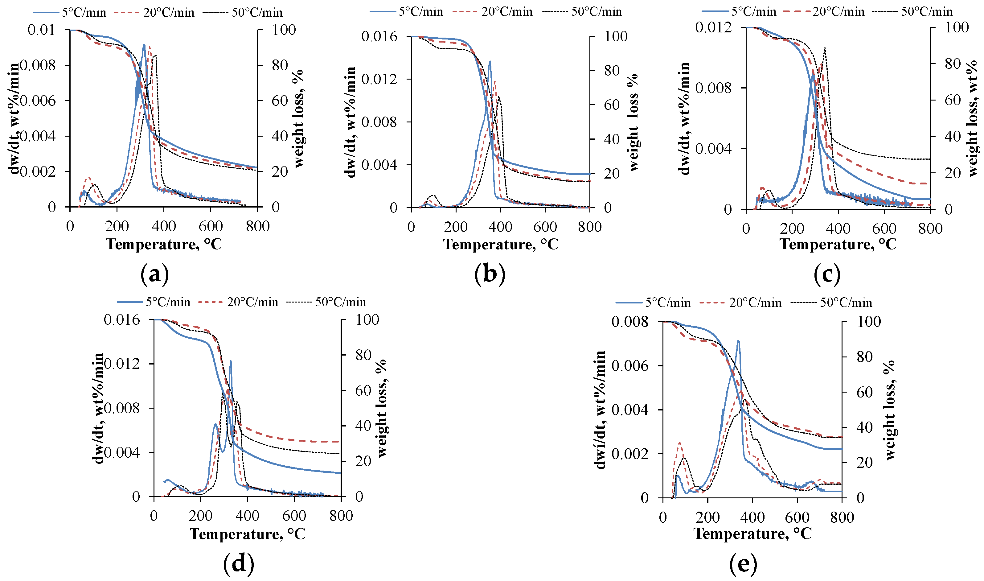
Thermogravimetric analysis provides significant information about biomass thermal behavior. The DTG curves give information about the decomposition steps; multiple peaks suggest several decomposition steps. Based on the literature, moisture content removal takes place under 200 °C, while devolatilization takes place under 600 °C and cracking or decomposition take place at higher temperatures of over 600 °C [25]. The TG and DTG curves of the used materials with a 5, 20 and 50 °C/min heating rate are depicted in Figure 1.

Focusing on the curves, it can be concluded that multiple steps appeared only in the case of the maize and piney biomass. Regarding the effect of the heating rate, a lower heating rate provides a higher decomposition rate and more ash. Moreover, the peak maximums were increased by almost 20 °C in each case with the increment in the heating rate. However, the lowest residual values were obtained with the 5 °C/min heating rate, which can be explained by the longer residence time, resulting in better heat conductivity; thus, the thermal degradation was more effective. The moisture content of the materials was eliminated in the following temperature ranges: 45–179 °C, 45–167 °C, 45–190 °C, 45–185 °C and 45–192 °C (in the same order as appears in the case of Figure 1). According to the results, the piney biomass contained the highest physisorbed moisture content. The decomposition of the volatilities took place in the ranges 167–566 °C, 167–528 °C, 190–553 °C, 185–538 °C and 192–615 °C, respectively, which gave the highest decomposition rate due to the high cellulose and hemicellulose content of the used materials. Above 600 °C, in the decomposition zone with char formation, a slight mass loss can be observed with different heating rates. The main parts of the lignocellulosic biomass decompose at different temperatures in the following order: hemicellulose (220–315 °C), cellulose (300–400 °C) and lignin (150–900 °C) [27]. Based on the mentioned phenomenon, in the case of the maize (Figure 1d) and piney (Figure 1e) biomass, the first peak indicates the hemicellulose, while the second indicates the cellulose content in the devolatilization zone. In the case of the piney biomass (Figure 1e), between 600 and 800 °C, a small peak appears, indicating the cracking or decomposition of the carbonaceous matter, which can be originated from the lignin content.

3.2. FTIR Analysis

The gases obtained during the TG analysis can be seen in Figure 2, as a function of temperature. The studied components are the carbon dioxide, carbon monoxide, H₂O, methane, aldehydes and ketones, alcohols and esters. The mentioned compounds can be identified as C=O (2400–2250 cm⁻¹), C-O (2250–2000 cm⁻¹), O-H (4000–3400 cm⁻¹), C-H (3000–2842 cm⁻¹), C=O (1800–1684 cm⁻¹) and C-O-H (1131–1058 cm⁻¹) functional groups [28]. Observing the FTIR spectra, it was noted that the individual peak temperatures appeared around 350–380 °C; moreover, the main degradation occurred between 200 and 600 °C, resulting in a great number of organic volatiles in the devolatilization/pyrolysis zone. Based on the results, it can be concluded that the carbon dioxide had the highest absorbance. The mentioned phenomenon can be explained by the breaking of the C-O and C-H chemical bonds, as well as the decarboxylation and decarbonylation of the hemicellulose units.

Regarding the CO₂, the peak intensity roughly follows the hemicellulose content of the raw materials as follows: sunflower husk ~ wheat > maize > industrial wood chips > piney biomass. It should be mentioned that carbon dioxide was also generated at higher temperatures with the piney biomass and sunflower husk. Concerning the CO, at lower temperatures, especially in the case of the piney biomass, it can be originated from the ether and carbonyl groups (phenylpropane units with weak internal linkages), while at higher temperatures it can be originated from the carboxyl and C-O groups of lignin together with char decomposition [29]. The appearing H₂O peaks between 45 and 192 °C represent the moisture content, while at over 205 °C they can be generated from the decomposition of the glycosidic hydroxyl groups of the hemicellulose and cellulose units. During the thermal degradation, methane mainly originated from the side chain and aromatic ring fracture of the lignin, as well as from the secondary reactions, which was remarkably abundant in the case of the piney biomass above 379 °C [30]. The aldehydes, ketones and acids can be originated from the cellulose and hemicellulose units, released mainly from the latter. Based on data in the literature, after the intramolecular dehydration of hemicellulose units, enol-keto tautomerization can occur from the glycosidic linkages between the monomer units, resulting in intermediates that can form acids, ketones and aldehydes during aromatization, decarboxylation reactions and intramolecular condensation [30,31]. Alcohols and esters are mainly produced from cellulose degradation, where the bonds between the β-1,4-glycosidic bonds broke, resulting in cellulose with a decreased polymerization degree and different monomers. The generated monomers after the rearrangement mostly form levoglucosan, alcohols and esters, which all appear at the same wavelength range (1131–1058 cm⁻¹) [30,31].

3.3. Kinetics and Thermodynamics

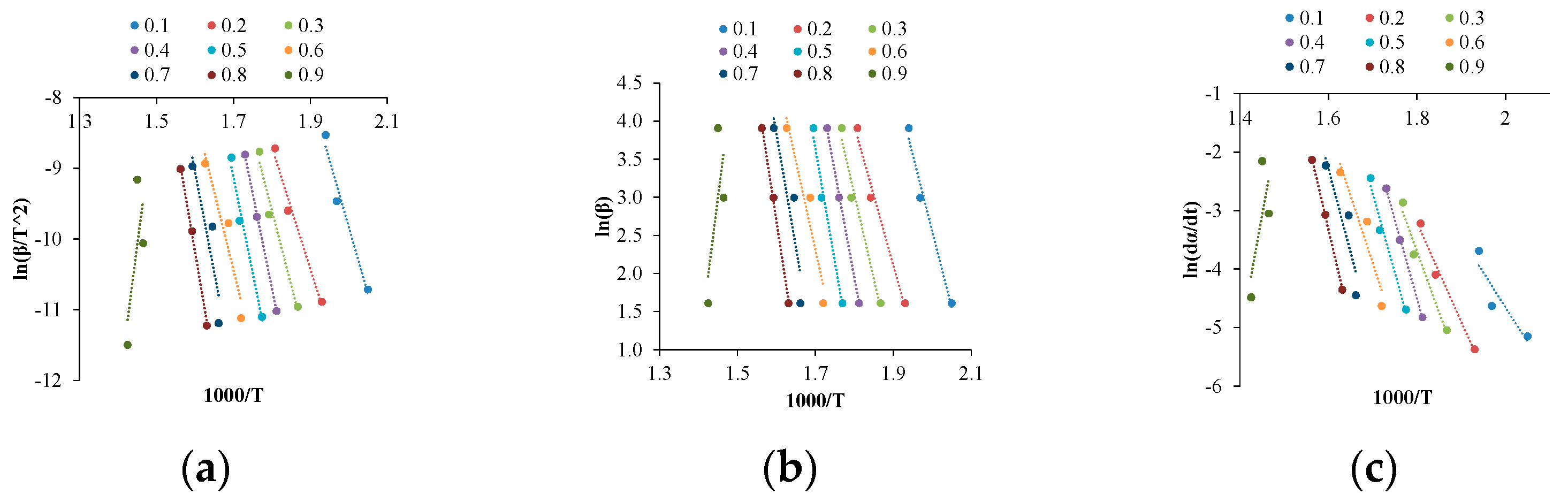
Firstly, the kinetic plots were obtained in the case of the different raw materials (Figure 3), where the data with 5, 20 and 50 °C/min heating rates from the thermogravimetric analysis were used. In Figure 3, the data obtained from the maize biomass are depicted; with different raw materials, the figures showed similar tendencies. Afterwards, the activation energy (

Table 2. Activation energy in kJ/mol with different model-free methods.

Conversion (α)	Maize			Sunflower Husk			Industrial Wood Chips			Wheat			Piney Biomass
	KAS	FWO	Friedman	KAS	FWO	Friedman	KAS	FWO	Friedman	KAS	FWO	Friedman	KAS	FWO	Friedman
0.1	349.4	158.9	98.2	115.9	101.8	199.6	264.7	242.9	266	98.8	82.1	96.8	34.9	26.7	39.5
0.2	269.1	144.1	141.4	287.6	282.3	286.2	288.6	283.3	288.1	245.7	223	244.8	72.1	67.5	73.4
0.3	237.8	174.6	173.6	242.7	237.9	242	210.8	209.6	210.5	321.1	314.7	321.1	70.8	68.5	70.6
0.4	184.7	221.6	223.1	184.5	184.6	184.1	233.5	231.4	233.5	234.3	232	234	68.4	66.6	68.3
0.5	442.7	429.6	441.9	196.4	195.9	196.1	233.5	228.8	230.7	222.3	220.4	221.9	61.8	61	61.8
0.6	223.9	184.9	192.2	193.9	193.7	193.8	211.3	210.7	211.5	213.8	212.2	213.3	89.6	89.6	89.4
0.7	174.6	235.5	237.8	201.8	201.5	202	189.7	190.4	190.2	190.1	189.5	189.3	87.4	87.8	87.7
0.8	142.8	265.5	268.7	286.7	264.5	285.8	172.9	174.5	173.5	144.5	145.8	143.3	125.3	121.3	125.5
0.9	157.2	321.1	347.9	183.5	162.1	181.1	624.1	603.8	624.9	188.3	186.6	185.8	218.6	194.9	215.8

) and the pre-exponential factor were calculated, with conversion values of between 0.1 and 0.9. The activation energy occurred from the slopes, while that of the pre-exponential factor was calculated from the increment in the slope with the different model-free methods that were mentioned earlier. Regarding the correlation coefficients, it can be noted that all the values were above 0.95, except the 0.1 (maize biomass and industrial wood chips) and 0.9 (wheat, maize and piney biomass) conversion values.

Based on the results, the reliability and comparability of the used methods is appropriate, owing to the negligible difference between the methods (in the case of the activation energy, its value is lower than 5%). Concerning the activation energy, it can be noted that it has a decreasing value with each method, with the exception of those conversion values where the correlation was under 0.9. Focusing on the average of the activation energy, the relation is the following: piney < wheat < sunflower husk < maize < industrial wood chips. Nevertheless, lower activation energy can occur due to free radicals, which can be generated from, e.g., aromatic groups of lignin. The range of the pre-exponential factor at different conversion values is relatively wide (109–1030 s⁻¹), which can be explained by the thermal degradation of the biomass, which indicates several complex chemical reactions.

Phuakpunk investigated corn cob pyrolysis with the TGA method, calculating the kinetic parameters with the FWO and Friedman methods. It was found that the activation energy was 110–250 kJ/mol, reaching the highest value at a 0.5–0.7 conversion value, which are the same values as in the case of the maize biomass that was investigated in this article [32]. With different heating rates of 10 °C, 20 °C and 30 °C, P. Thenmozhi investigated the pyrolysis of corn cob, where the activation energy changed between 95.7 and 169.0 kJ/mol, reaching the highest values at a 0.5 conversion value [33]. Regarding degradation, in both articles it occurred in two or three different steps.

Rathore investigated the kinetic analysis and thermal degradation of wheat straw with KAS, FWO and Starink methods, utilizing 900 °C end temperature with 20 °C/min, 30 °C/min and 40 °C/min heating rates. It was noted that the main degradation step was occurred between 180 and 430 °C. Regarding the E_a, the main values were 125–193 kJ/mol obtained from FWO, KAS and Starink models in the conversion range of 0.1–0.8 [34].

The thermodynamic parameters (

Table 3. Thermodynamic parameters with different model-free methods (KAS, FWO, Friedman), in the case of maize biomass.

	KAS			FWO			Friedman
Conversion (α)	dH, kJ/mol	dG, kJ/mol	dS, J/molK	dH, kJ/mol	dG, kJ/mol	dS, J/molK	dH, kJ/mol	dG, kJ/mol	dS, J/molK
0.1	183.2	155.2	45.5	181.5	80.1	164.8	180.6	131.0	80.6
0.2	139.4	186.2	−76.2	140.7	113.0	45.0	138.2	158.7	−33.4
0.3	185.0	187.5	−4.1	184.4	112.0	117.5	184.2	208.5	−39.5
0.4	208.7	190.0	30.3	207.0	113.3	152.3	208.1	158.4	80.9
0.5	217.2	194.8	36.3	215.3	117.7	158.7	216.8	162.1	88.9
0.6	229.1	199.9	47.5	226.9	122.2	170.2	228.9	166.2	101.9
0.7	316.0	206.4	178.1	309.6	124.4	301.1	316.0	171.9	234.1
0.8	240.6	118.5	198.6	217.9	172.5	73.8	239.7	153.6	140.0
0.9	93.7	119.5	−42.0	77.0	180.7	−168.7	91.7	155.1	−103.1

) such as enthalpy, Gibbs free energy and entropy were determined from the activation energy and the pre-exponential factors. Regarding the enthalpy, it can be noted that the average difference was relatively low, which can be explained by the easy product formation. The Gibbs free energy gives information about the formation of active complex, whose value was commonly in a narrow range except at the 0.1 and 0.9 conversion values, where the correlation was not adequate.

Concerning the entropy, negative values can be found at different conversion values, which leads to a molecular structure that is more organized compared with the original ones [29]. Regarding the thermodynamic parameters, with different model-free methods, the enthalpy values have a maximum of 10% difference in the case of the different raw materials at 0.1–0.9 conversion values. However, the calculation of Gibbs free energy requires not only the activation energy, but the pre-exponential factor and also the Planck and the Boltzmann constant. Moreover, the value of the pre-exponential factor is relatively wide, which results in different Gibbs free energies. The entropy can be evaluated with the enthalpy and Gibbs free energy, giving quite different entropy values in the case of the diverse model-free methods.

The kinetic and thermodynamic data of the different raw materials with a wide range (0.1–0.9) of conversion values give information on the thermochemical conversion processes during the degradation; they also provide data for the scale-up processes.

3.4. Modeling of TG Process and Temporal Evolution of Gas Composition

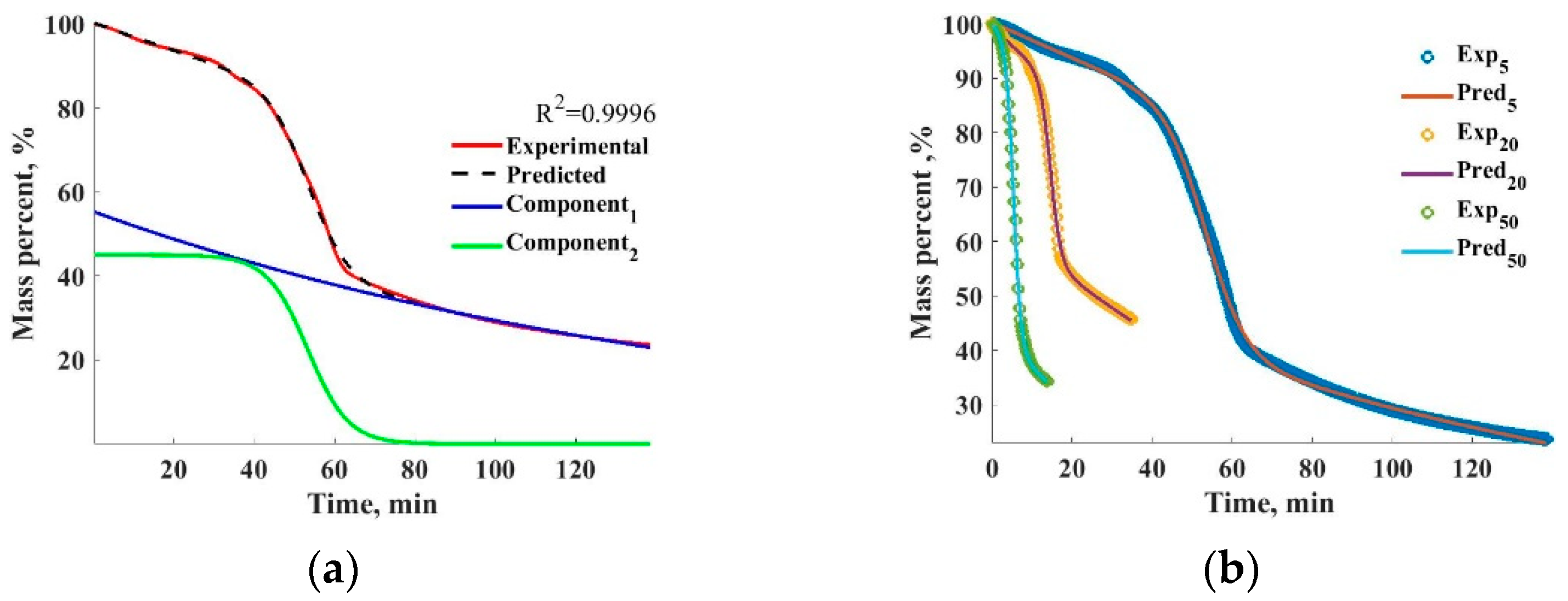
As mentioned previously, the logistic mixture and ARX models will be presented for the prediction of TG-FTIR profiles as well as the gas composition, as shown in Section 2.4. The results will be showcased using the data set of the maize TGA but can be generalized for all the investigated materials. The experimental and predicted TGA profiles using the logistic mixture model detailed in Section 2.4 and can be seen in Figure 4a with c = 2 and n = 1. The fit managed to achieve a corrected R² score of over 0.99. The two component logistic functions used to create the mixture model are displayed as well. It can be seen that the model accurately captures the TGA tendencies and the two components may be indicative of overlapping processes during the degradation.

The fit accuracy as a function of the component number and polynomial order was investigated to establish the optimal model structure. The average R² scores of the three registered TGA curves were compared to make a choice. The average R² scores of the fit to the maize data set were used under a different mixture model component number and polynomial order. When the polynomial order = 1, 2, 3, the number of the mixture model component can be changed similarly between 1 and 3, where the average of R² scores is increased by the higher polynomial order, reaching 0.9997–0.9998, while in the case of the lower values the fitting is more imprecise (0.9339–0.9873). As the results showed, the mixture model with a component number of 2 and a polyonimal order of 1 produced fit scores of over 0.99 on average; further increments in either the polynomial order or component number did not result in significant increments in the fitting accuracy. Therefore, for the maize data set, the parameters c = 2 and n = 1 were chosen for all the heating profiles, resulting in a simple but accurate model structure of the process.

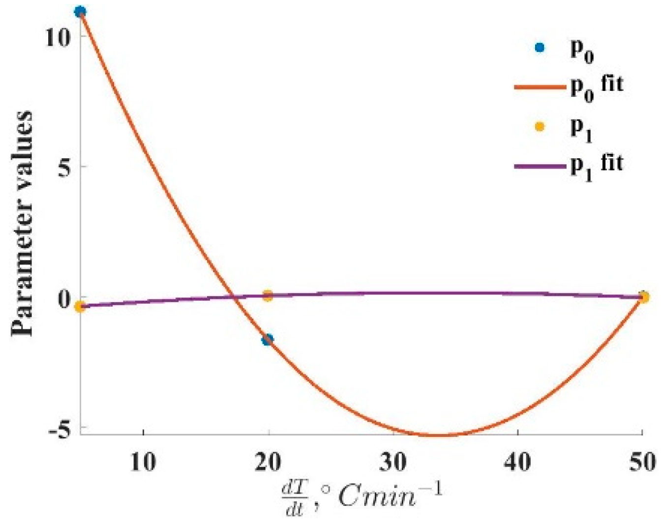
The fitting results for the three investigated heating rate cases are shown in Figure 4b. In order to predict the impact of the heating profile on the TGA results, a second-order polynomial equation has been fitted to the optimized parameters. This way, a link between the heating speed and the parameters of the logistic mixture model was obtained and can be used to predict the heating profiles of the intermittent heating rates. The optimized parameters of the logistic mixture model as a function of the heating rate are displayed in Figure 5, with the addition of the fitted polynomial function.

The parameters of the polynomial equations to estimate the components of the logistic mixture model are provided in

Table 4. Polynomial equation parameters for estimation of the logistic mixture model components.

Parameters of the Logistic Mixture Model Components		Constant	Linear	Quadratic
Component 1	$p_0$	10.93	−1.62	0.0260
	$p_1$	−0.34	0.07	−0.0009
	$w_1$	2660	−184	2.6400
Component 2	$p_0$	−17.49	1.50	−0.0222
	$p_1$	0.29	−0.02	0.0003
	$w_2$	1280	291	−5.1530

. For each parameter (p₀, p₁, w₁ and w₂), there are a constant, a linear and a quadratic value for the calculations. In the case of all the components, $w_i$ is the weight of each logistic function in the mixture, while $p_i$ is the corresponding fitting parameter.

As mentioned above, the fitting of the ARX model was controlled by MATLAB R2020a, where the optimized parameters were minimized by the sum of the squared errors using the Broyden–Fletcher–Goldfarb–Shanno algorithm.

The absorbance values of CO₂, CO and CH₄ have been fitted using an ARX model, which can be seen in Figure 6a. The fitted model was a sixth-order ARX model with good fit accuracy (R² = 0.9988). For the modeling, the data were separated in a 70–30% cut into training and test data; the cut-off is denoted by a red line in Figure 6a, with the validation data being the later registered absorbance values.

The model order was chosen by observing the distribution of the fit error auto-correlation function. The auto-correlation function of the fit error can be seen in Figure 6b. At a model order of 6, the distribution of the error auto-correlation function corresponded mostly to a white noise sequence, pointing to a good fit with small bias and variance. Further increments in the model order resulted only in small changes within the error auto-correlation function and an increment in fit result variance and were thus omitted.

The parameters of the optimized ARX model are summarized in

Table 5. Regression coefficients of the ARX model.

Model Parameters		CO2	CO	CH4
X component	$p_0$	1.58 × 10−4	7.01 × 10−4	6.57 × 10−5
	$p_1$	−1.06 × 10−5	6.92 × 10−4	−5.11 × 10−5
	$p_2$	−2.23 × 10−4	−0.01	−1.27 × 10−4
	$p_3$	1.62 × 10−4	2.72 × 10−4	1.43 × 10−4
	$p_4$	−2.33 × 10−4	7.00 × 10−4	1.38 × 10−5
	$p_5$	2.53 × 10−4	2.12 × 10−4	−3.38 × 10−5
	$p_6$	−9.48 × 10−5	−2.72 × 10−4	−1.05 × 10−5
	$p_7$	0.11	0.24	0.17
AR component	$x_0$	0.03	0.06	−0.11
	$x_1$	−0.07	0.99	−0.02
	$x_2$	−0.19	−0.02	−0.19
	$x_3$	−0.04	0.04	0.50
	$x_4$	−0.02	−0.53	0.07
	$x_5$	−0.27	−0.13	0.03
	$x_6$	0.02	−0.22	0.02
	$x_7$	0.01	−1.27	0.52

. The AR components (previous instances of component absorbance) as well as the exogeneous components (sample weight instances) are listed and their weighting parameters is given.

4. Discussion

During the decomposition of the five different biomass with TG-FTIR, the individual peaks of CO₂, CO, H₂O, CH₄, aldehydes and ketones, alcohols and esters were studied, with an investigation of the kinetic parameters and model fitting. The thermogravimetric analysis gave insights into the biomass thermal behavior, where diverse decomposition steps were observed, resulting in multiple peaks with the indication of various degradation stages. Moreover, the moisture content removal and volatility decomposition temperatures were defined, providing valuable information on the biomass composition and behavior.

Throughout the FTIR spectroscopy, the peak temperatures for the component decomposition and highlighting of the main degradation ranges were identified. The dominance of carbon dioxide could have originated from the decarboxylation reactions. Additionally, the FTIR spectra help to identify the various functional groups associated with gas production, considering the chemistry of biomass decomposition.

The kinetic analysis revealed temperature-dependent activation energies and pre-exponential factors. Despite the minor divergence among the different model-free methods, the isoconversional methods produced similar data. The logistic mixture and ARX models are introduced for predicting the TG-FTIR profiles and gas composition, with the results demonstrated using the maize TG data but applicable to all the studied materials. The logistic mixture model achieved a corrected R² score exceeding 0.99, accurately capturing the degradation tendencies with two indicative components. Additionally, a second-order polynomial equation connects the heating rate to the logistic mixture model parameters, promoting the prediction of the TG results for different heating rates.

5. Conclusions

In this study, the decomposition behavior of various biomass samples was investigated using TG-FTIR up to 800 °C, with heating rates of 5, 20 and 50 °C/min. A shift in peak maximums was observed by approximately 20 °C with the increment in heating rates. The DTG curve analysis revealed distinct decomposition patterns, especially in the case of the maize and piney biomass, which resulted in two decomposition peaks. During the FTIR analysis, individual peaks of the studied components between 350 and 380 °C were identified, with primary degradation occurring broadly between 200 and 600 °C. These temperature ranges offer insights into the underlying mechanisms that are significant in optimizing the thermochemical conversion processes and the quality of products.

Regarding the alternative kinetic modeling, the logistic mixture models exhibited promising fitting performance, with R² = 0.9988 values for the validation data. This suggests their potential as a robust tool for characterizing complex degradation processes, opening opportunities for future research into biomass utilization. The kinetic and modeling results help to understand the decomposition of biomass through techniques like TG-FTIR, which inform the development of efficient thermochemical conversion processes. Moreover, they give an insight into kinetic modeling, promoted with logistic mixture models, enhancing the predictive capabilities for further process optimization, with the minimizing of environmental impacts.